Abstract
Effective machine learning regression models are useful toolsets for managing and planning energy in PV grid-connected systems. Machine learning regression models, however, have been crucial in the analysis, forecasting, and prediction of numerous parameters that support the efficient management of the production and distribution of green energy. This article proposes multiple regression models for power prediction using the Sharda University PV dataset (2022 Edition). The proposed regression model is inspired by a unique data pre-processing technique for forecasting PV power generation. Performance metrics, namely mean absolute error (MAE), mean squared error (MSE), root mean squared error (RMSE), R2-score, and predicted vs. actual value plots, have been used to compare the performance of the different regression. Simulation results show that the multilayer perceptron regressor outperforms the other algorithms, with an RMSE of 17.870 and an R2 score of 0.9377. Feature importance analysis has been performed to determine the most significant features that influence PV power generation.
1. Introduction
Due to the capacity to produce power without predominantly generating greenhouse gases, photovoltaic (PV) systems are being considered as an alternative form of clean energy. Precise PV power generation forecasts are crucial for effective electricity oversight, particularly for establishing and programming purposes [1]. Reliable forecasting of power generation, impacted by an assortment of variables, including the climate, radiation from the sun, and system effectiveness, is necessary for the effective operation of PV systems [2]. Accurate forecasting is crucial for effective energy management, planning, energy generation scheduling, and ensuring the power grid’s stability and reliability [3]. In recent years, conventional machine learning algorithms have emerged as powerful tools for forecasting PV power generation. Demand response, proactive maintenance, energy production, and load predicting are just a few applications where machine learning models are the go-to toolkit for researchers [4]. These models can capture complex nonlinear relationships between various factors influencing power generation and accurately predicting future values [5]. The use of deep learning, nevertheless, can be useful when dealing with time series data. Auto-Regressive Integrated Moving Averages (ARIMAs) methods are beneficial for instantaneous forecasting of powerful time series data. Artificial neural networks are far more potent than ARIMA models and quantitative approaches, particularly for modeling complicated interactions [6]. Because artificial neural networks have the appropriate properties for interacting with non-linear models, forecasting time series has become a more common application for supervised neural networks in recent years. Estimating PV output can be crucial for grid operators and energy providers to plan and optimize tasks like managing maintenance and regulating power demand. Machine learning regression models can offer forecasting and anomaly detection in PV plants in such cases. In this study, multiple regression models, such as linear regression (LR), a support vector regressor (SVR), a k-neighbor regressor (KNR), a decision tree regressor (DTR), a random forest regressor (DFR), a gradient boosting regressor (GBR), and a multilayer perceptron regressor (MLP), have been used for PV power generation forecasting with promising results [7]. The effectiveness of the proposed regression model has been compared with existing approaches.
1.1. Motivation and Contribution
To address the effectiveness and applications of regression models for forecasting PV power generation, a comparative analysis of multiple regression models used on a dataset has been proposed. The testbed architecture of the PV system installed in the SHARDA University campus is discussed in Figure 1 of the manuscript, followed by the dataset description. Some of the major contributions of the article are as follows:
- Realistic time series dataset is harvested from PV panels (with sensors) and installed on multiple buildings of the SHARDA University campus.
- A comparative study and a performance analysis of the LR, SVR, KNR, DTR, RFR, GBR, and MPR for power prediction are tested.
- A discussion of numerous case studies for PV power is presented to identify the important features favoring power prediction.
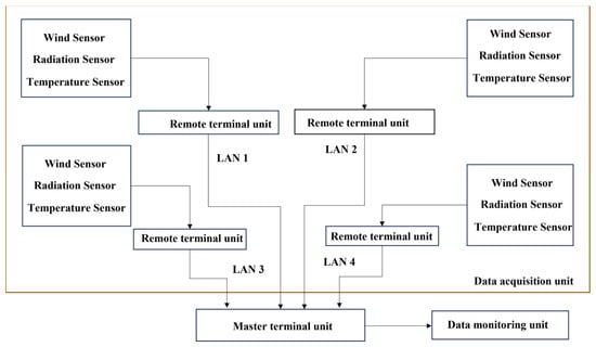
Figure 1.
Testbed architecture of PV system at Sharda University.
Figure 1.
Testbed architecture of PV system at Sharda University.
1.2. Acronyms Used
The abbreviations and short forms used throughout the article are presented in Table 1 of the manuscript.

Table 1.
Abbreviations and short forms.
1.3. Structure of the Article
The structure of the manuscript starts with the introduction containing the research statement, problem identification, and improvements required. The introduction contains three subsections: the first subsection represents the motivation and contribution; the second subsection presents acronyms used throughout the manuscript; and the third subsection depicts the structure of the manuscript. Section 2 of the manuscript presents a detailed literature review of the related articles. Section 3 of the manuscript depicts the Testbed architecture with a dataset description. The Data Acquisition Unit and Data Monitoring Unit (DTU) are the two core subsections of Section 3. Section 4 of the manuscript describes the proposed methodology, with various data preprocessing steps and multiple regression methods. Section 5 of the manuscript discusses the results obtained from two case studies, which are Case 1 and Case 2. Section 6 highlights a comparison of existing state-of-the-art regression modelling for PV power prediction. Section 7 of the manuscript presents the conclusion and future scope of the proposed research methodology.
2. Literature Survey
In this section, a literature survey has been conducted based on relevant research conducted in PV power forecasting using XAI and machine learning regression models. Table 2 presents the current state of the art research, including recent research in the field of PV power forecasting with the help of regression modeling.
Table 2.
Background and literature review.
3. Testbed and Dataset Description
The dataset utilized in this study has been obtained from the data collection Centre at SU in Uttar Pradesh, India 28.4753° N, 77.4823° E, which is dispersed across several building rooftops. The dataset contains the records of the year (2022) from date 21 January 2022 to 21 December 2023, and it has a time-lapse of 15 min between each instance. The dataset has seven features namely hour, power (kW), irradiance (W/m2) (IRR), wind (km/h), ambient/panel temperature (°C), and PR representing performance percentage.
The architecture of the PV system is given in Figure 1 of the manuscript below, where the PV panels are distributed at several locations. Various subparts of the testbed have been discussed in detail in Section 3.1.
3.1. DAQ Unit
The DAQ unit and DMU are the main components of the chosen test bed. PV panels are installed at various locations on the building rooftops of various buildings on the SU campus. In addition, PV panels are equipped with radiation sensors, wind sensors, and temperature transmitters. All the installed sensors transmit data to the remote terminal unit.
3.2. DMU
The DMU is used as a strong surveillance system to guarantee the steady and dependable performance of any PV system. The DM unit also monitors several electricity production indices and fault occurrences. In the proposed system, data from RTUs are transmitted to a sub-control system, equipped with computer-aided monitoring for data generation and system monitoring.
4. Proposed Regression Methodology
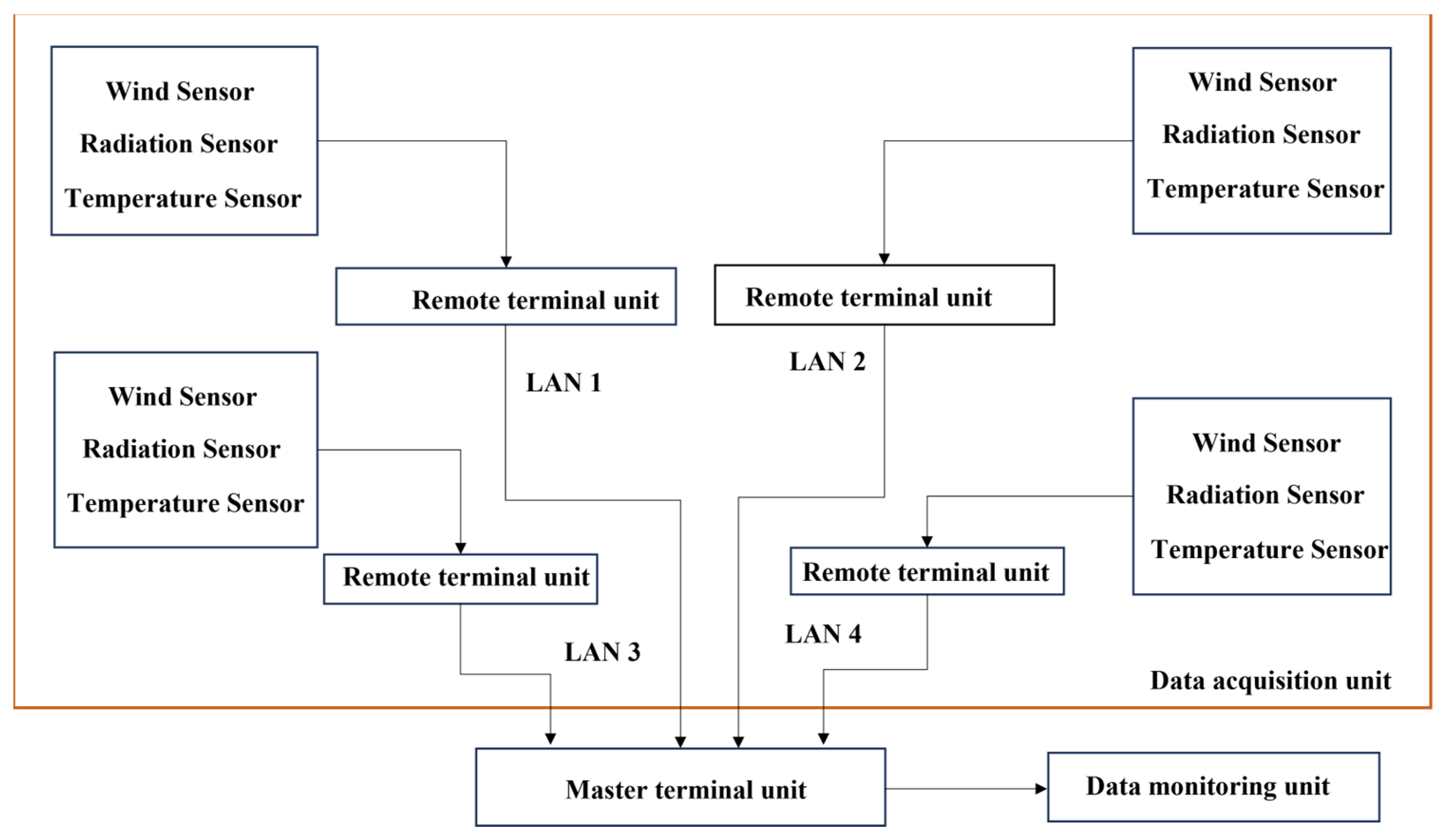
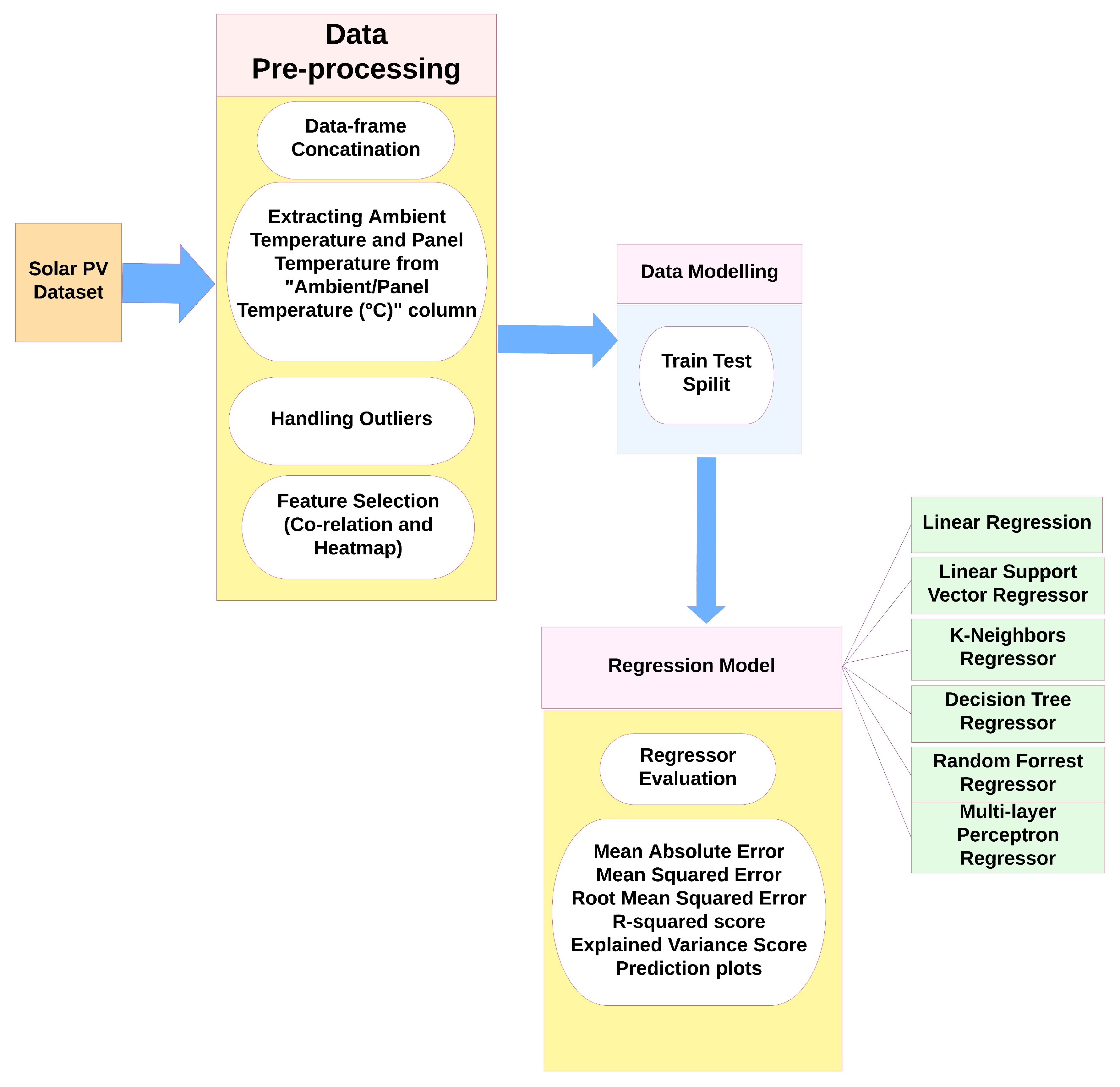
The various building blocks of the proposed model are presented in Figure 2. It starts with taking the PV dataset as the input and performs multiple preprocessing steps on it. The preprocessed data frame is directed for data modeling and to the selected regressor at the end.
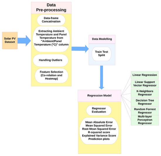
Figure 2.
Proposed regression model.
4.1. PV Dataset
The dataset used in this study was collected from multiple building rooftops at the SU data collection Centre in Uttar Pradesh, India (28.4753° N, 77.4823° E). With a time gap of fifteen minutes between each occurrence, the dataset includes the recordings for the year 2022 from 21 January 2022 to 31 December 2023. The dataset includes the following seven features: wind speed (km/h), power (kW), hour, ambient/panel temperature (degrees Celsius), irradiance (W/m2) (IRR), and PR, or performance percentage.
4.2. Data Pre-Processing
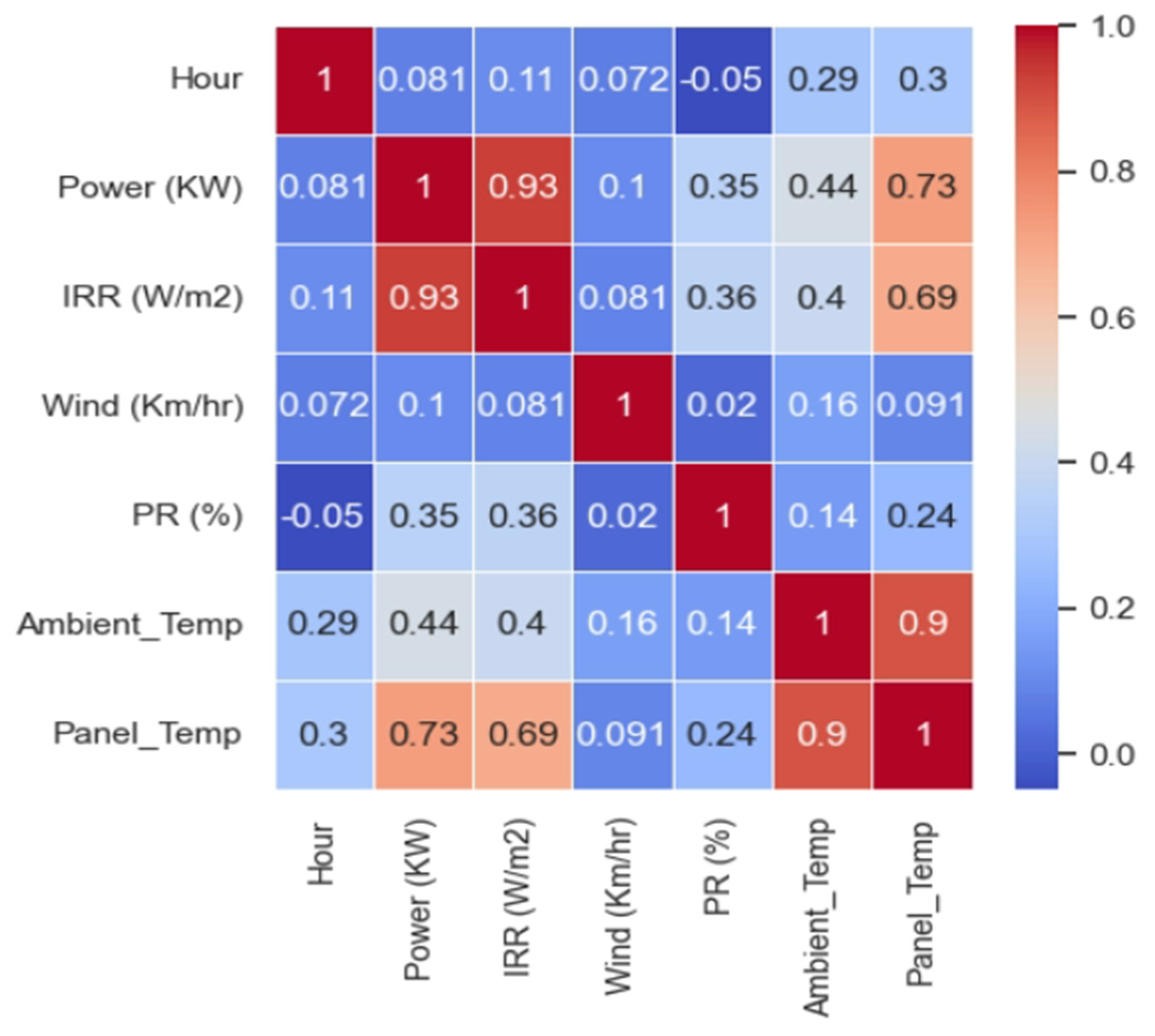
In response to the data distribution within the six features, the pre-processing steps embedded with regression models are depicted in Figure 3. The proposed regression model takes the PV dataset as input and dataset concatenation is an initial step taken towards pre-processing. After data-frame concatenation, the column “Ambient/Panel Temperature (°C)” is separated into ambient Temperature and panel temperature columns. Before feature selection, outliers are detected and handled within the data frame with normalized values. Furthermore, a correlation and heat map have been used to select important features and drop redundant features as shown in Figure 3. In the proposed work, two case studies have been considered for data analysis.
Case 1:—Data frame with all features and removing rows with Null (NaN) values.
Case 2:—Data frame without PR% and wind (km/h) feature.
The two case studies have been deliberated in Section 5 of the manuscript.

Figure 3.
Pearson correlation and heat map of data frame.
Figure 3.
Pearson correlation and heat map of data frame.
4.3. Data Modelling
The data frame is divided into training and testing, with 80% for training and 20% for training. Power feature is selected as the target feature.
4.4. Regression Models
Various regression models have been used to predict the power production from the data. The performance of each of the regression models used is evaluated using MAE, MSE, RMSE, R2 error, explained variance score, and prediction plots. Considered regression models have been explained in Section 4 hereafter.
4.4.1. Linear Regression
The strategies in linear regression assume that the desired result will be a linear blend of the attributes. If ỹ represents the anticipated value in the notated form, it may be given as
ỹ(W,X) = W0 + W1 × 1 + W2 × 2 + … WnXn
The shape of the vector is w = (W1, W2, … Wn) as the coefficient and W0 as the intercept throughout the function. To reduce the total of the residuals of squares among the targets found in the data frame and the ones forecasted using the linear estimation, linear regression builds an equation with coefficients W = (W1, W2, … ,Wn−1, Wn).
4.4.2. Support Vector Regressor
It is comparable to SVR, which uses the argument kernel = ‘linear’, but because it is constructed using “liblinear” instead of “libsvm”, it offers additional versatility in the selection of penalty and loss coefficients and can expand more effectively to large chunks of data samples. The input of both kinds is supported using this method [22].
For a trained dataset, if X is the input data and Y is the target variable, SVR aims to find coefficients a and b that minimize the cost function and can be illustrated as
|a| = norm of the weight vector a; C = regularization parameter; L = loss function that penalizes errors.
4.4.3. K-Neighbor Regressor
The idea underlying nearest neighbor approaches is to select a set with several training instances that are situated most closely to the point of interest and subsequently estimate the designation based on them [23]. Regarding the scenario of radius-based neighbor learning, the number of observations can either rely on the regional concentration of points or be a customized constant (k-nearest neighbor learning). The distance can normally be expressed in any metric system unit; the most popular option is the conventional Euclidean distance. Since neighbors-based strategies merely “remember” everything about the training data instances, they are referred to as non-generalizing machine learning approaches [24]. Regression and time series prediction, where the desired factor is often an order of interval scaled values, can benefit from applying the k-NN classifying concept when the reliant parameter is categorical [25].
For a single input sample, a, the predicted output b is calculated as the average of the target values of the K nearest neighbor in the dataset and can be illustrated as
here, is the predicted output for input a, bi is the target value of the i-th nearest neighbor, and k is the no of neighbors.
4.4.4. Decision Tree Regressor
A decision tree regressor develops a model in the form of a tree structure to estimate data in the future and generate useful continual output by observing the properties of an item. Seamless output denotes the absence of uniform output, i.e., the absence of representation by a discrete, well-known set of values [26]. The number of observations that must have been collected for a tree to contemplate shattering a node into two is known as the minimum sample split parameter. A structure splits until it reaches this value. The level of a decision tree needs to be maintained constantly because a shallower tree is going to possess significant bias along with little variance, whereas a more extensive tree would have high variance and low bias [27,28]. As a result, in our study, we tested using the splitting criterion as well as the maximum depth of the tree to generate a model that is as accurate as possible. The mathematical representation of a decision tree regressor is illustrated in
here
- represents predicted output for the input a using a decision tree.
- Ci is the constant value associated with the leaf node i.
4.4.5. Random Forest Regressor
Three primary phases make up the random forest development algorithm. Establishing B sample sets of dimensions N utilizing the baseline data, these sample sets might be swapped out and combined. For every sample in the dataset, we create a random forest tree Tb by iteratively continuing the subsequent procedures for each terminal node unless the minimal node count min is obtained:
- Pick m predictors randomly from the p covariates.
- Choose the top predictor for the split section out of the m identified predictors.
- Divide this location (node) into two minor nodes by establishing specific decision-making guidelines.
Lastly, determine the combination of the trees , where B is the total number of trees in the random forest.
- is the predicted output for the input X;
- B is the total number of trees left (base learners right) in the RFR
- is the prdiction of the b-the decision tree in the forest for input X.
The final prediction is the average of these individual tree predictions.
4.4.6. Gradient Boosting Regressor
The loss argument in the gradient boosting regressor allows the specification of a variety of loss functions in regression and squared error, which constitutes a typical loss function. A loss function is employed during the boosting procedure. The “squared error” and “Poisson” losses incorporate the “half least squares loss” and “half Poisson deviance” to make the mathematical calculation of the gradient simpler. Additionally, “Poisson” loss employs an internal log connection and needs y ≥ 0. Pinball loss is employed by “quantile”.
Mathematical representation for M weak learners and the prediction FM(i) for input (i) is given using
FM(i) is the predicted output for (i) input using a gradient boost model with weak learners. is the prediction of the m-th weak learner for input (i), and is the weight assigned to the m-th weak learner. The update rule for the weights and the new weak learner is determined by minimizing a loss function, often using gradient descent.
4.4.7. Multilayer Perceptron Regressor
MLP has a layered configuration with input, hidden, and output layers, like the other neural networks. During the MLP classifier’s recurrent development process to adjust the parameters, the estimates of the loss function regarding the parameter estimation are generated at each observation time. The loss function may undergo a convolution operation that lowers the model’s coefficients to prevent overfitting [29]. It learns with a supporting function.
where “” represents the input space, “” indicates mapping from the input space to the outer space, represents the outer space [30]. A data frame with the input X = ( and the target variable and y is provided. “” represents the input space, “” indicates mapping from the input space to the outer space, represents the outer space [30]. The proposed MLP regressor is tuned with Adam as an optimizer, and loss is calculated using MAE and with a learning rate parameter of 0.01, across 250 epochs. The decimal value of 0.31 is used as the initial value for the validation split parameter on the training set of data. The information from the preceding layer is transformed by each neuron in the hidden layer using a weighted linear sum of weights and input sets.
5. Results
For the proposed model, the results section is divided into two case studies concerning the feature vector of the dataset. Pearson’s correlation method has been used to select and drop the features from the dataset. Pearson’s correlation method is simple and strategic to determine the strong and weak correlation between independent and dependent variables [31]. From Figure 4 of the manuscript, which is the correlation and heat map plot of the features, wind (km/h) and hour are visualized as weakly correlated and are dropped in two different cases. The two different case studies are
Case 1:—Data frame with all features and removing rows with null (NaN) values.
Case 2:—Data frame without PR% and wind (km/h) feature.
For each case study, the LR, SVR, KNR, DTR, RFR, MLP, and GBR are tested. The performance of each regression model is evaluated using the MAE, MSE, RMS, R2 Score, and prediction plots (actual and predicted values).
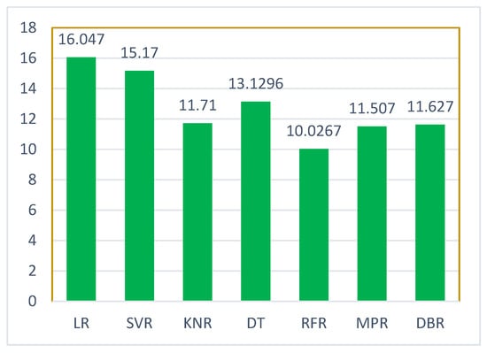
Figure 4.
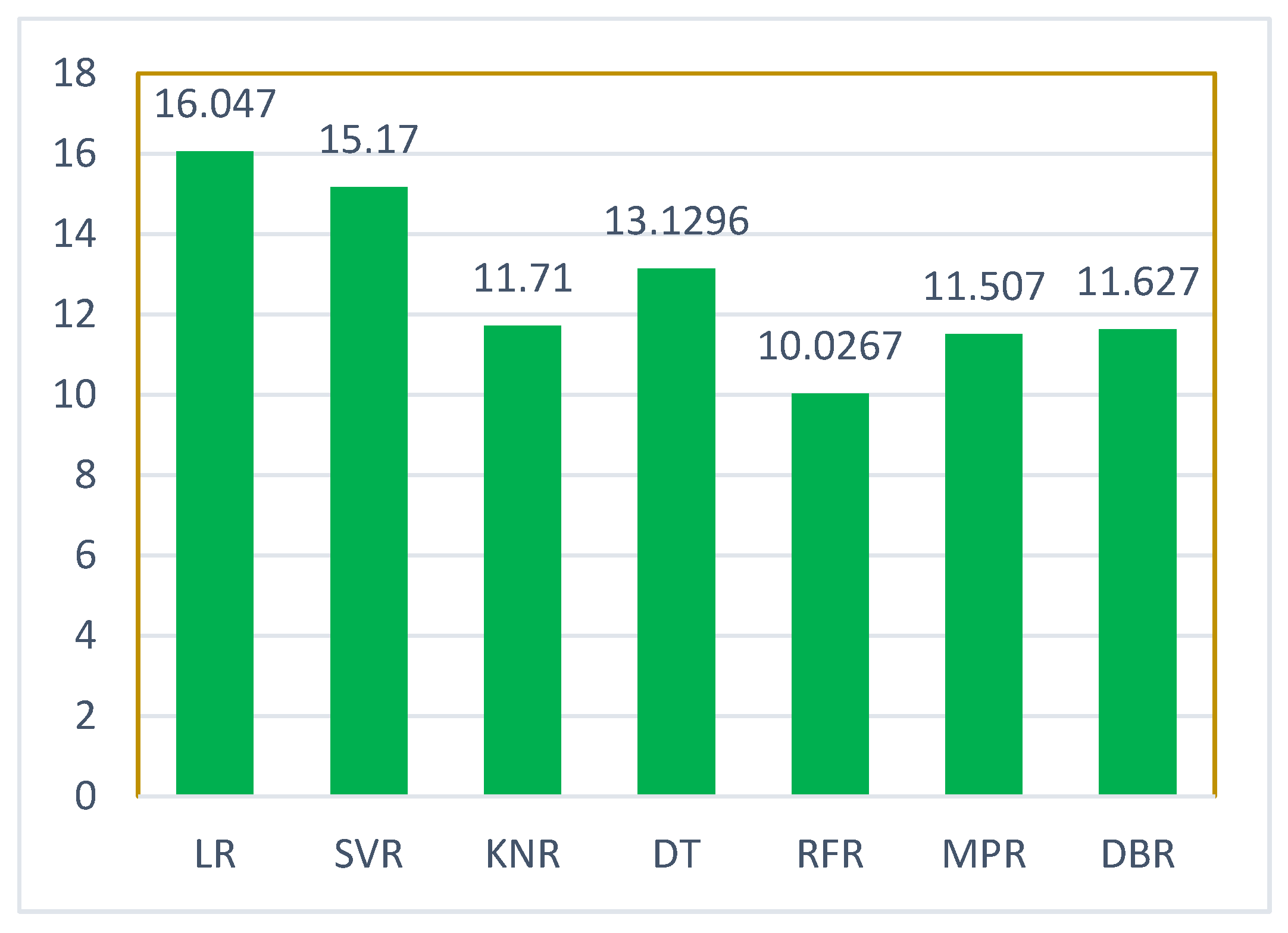
MAE score plots of Case 1.
Figure 4.
MAE score plots of Case 1.
5.1. Case 1:—Data Frame with All Features
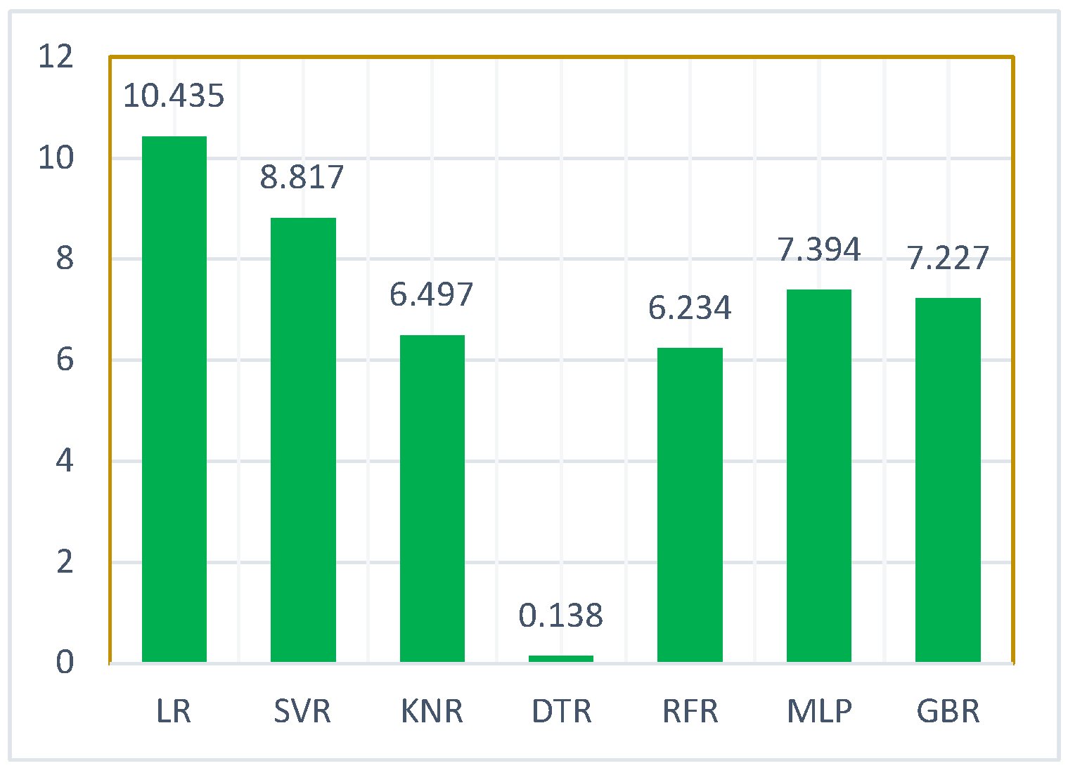
The PR% feature of the dataset contains a hefty amount of NaN values, so all NaN-valued rows from it have been dropped. Time slots during the night were all representing NaN values in the PR% column. Replacing NaN values with substitute statistical outcomes was not an option and could have inserted bias in the dataset. However, the power generation using the PV system at night is zero. In this case study, the rows representing NaN in the PR% column are dropped. A comparison of various errors for Case 1 using the regression method has been presented in Table 3. and score plots for the MAE, MSE, RMSE, and R2 are illustrated in Figure 4, Figure 5, Figure 6 and Figure 7. The comparison of actual values and prediction values for Case 1 using various models is plotted in Figure 8, Figure 9, Figure 10, Figure 11, Figure 12, Figure 13 and Figure 14.
Table 3.
MAE, MSE, RMSE, and R2 error outcomes in Case 1.
The efficacy and performance of the various ML regression models are presented in the form of MAE, MSE, RMSE, and R2 scores. Figure 4 of the article depicts the MAE scores obtained from various regression methods. The vertical axis represents the numeric values ranging from 0 to 18, and the values of MAE obtained using each regressor model are presented in the plot.
In contrast, Figure 5 depicts the MSE scores obtained from various regression methods. The vertical axis represents the numeric values ranging from 0 to 700, and the value of MSE obtained using each regressor model is presented in the plot.
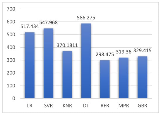
Figure 5.
MSE score plots of Case 1.
Figure 5.
MSE score plots of Case 1.

Similarly, Figure 6 depicts the RMSE scores obtained from various regression methods. The vertical axis represents the numeric values ranging from 0 to 700, and the values of RMSE obtained using each regressor model are presented in the plot.
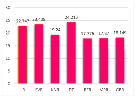
Figure 6.
RMSE score plots of Case 1.
Figure 6.
RMSE score plots of Case 1.
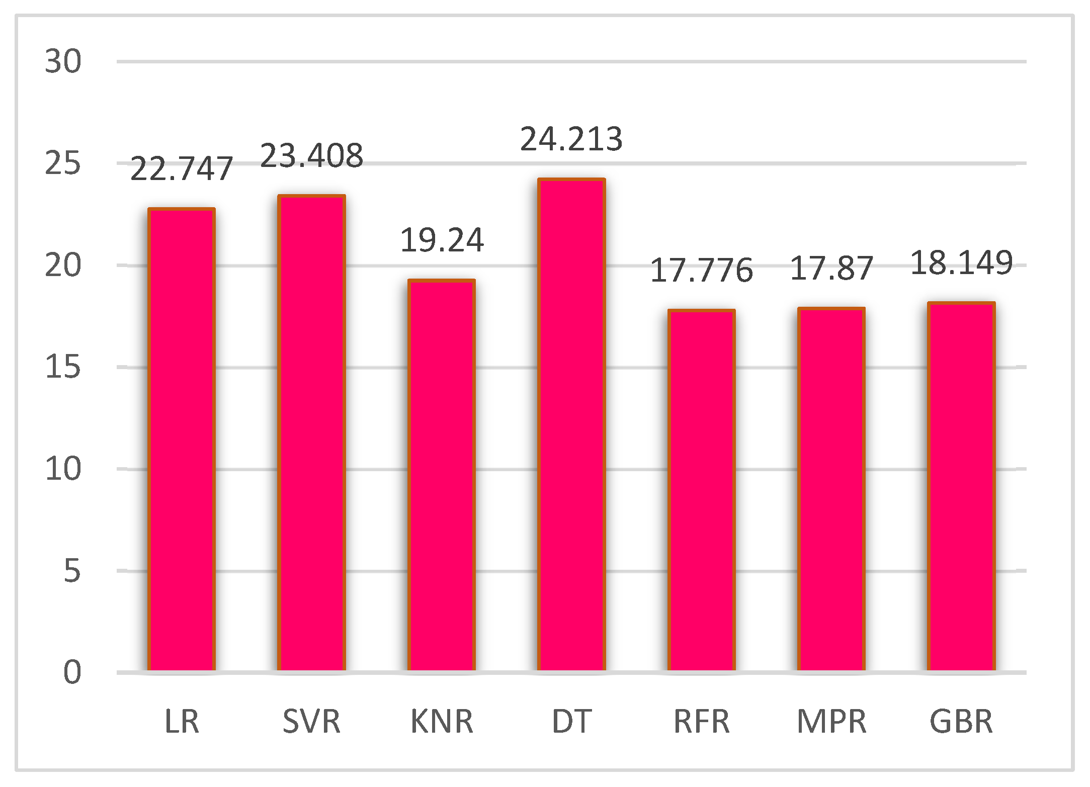
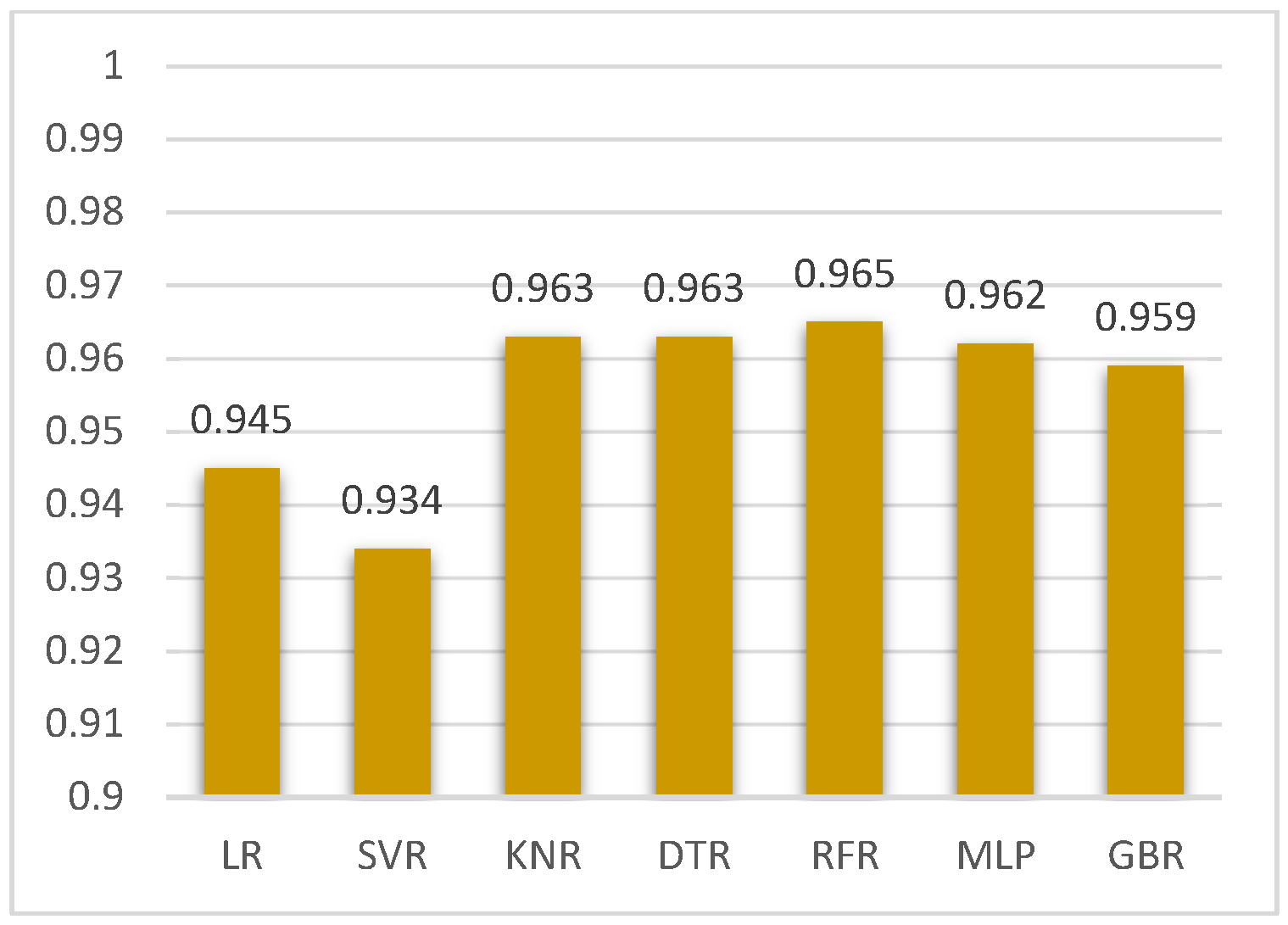
Figure 7 of the study illustrates the R2 values acquired from numerous regression approaches. The vertical axis indicates the numeric values ranging from 0.82 to 1.0, and R2 values obtained using each regressor model are shown in the plot.
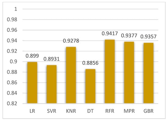
Figure 7.
Root square error score plots of Case 1.
Figure 7.
Root square error score plots of Case 1.
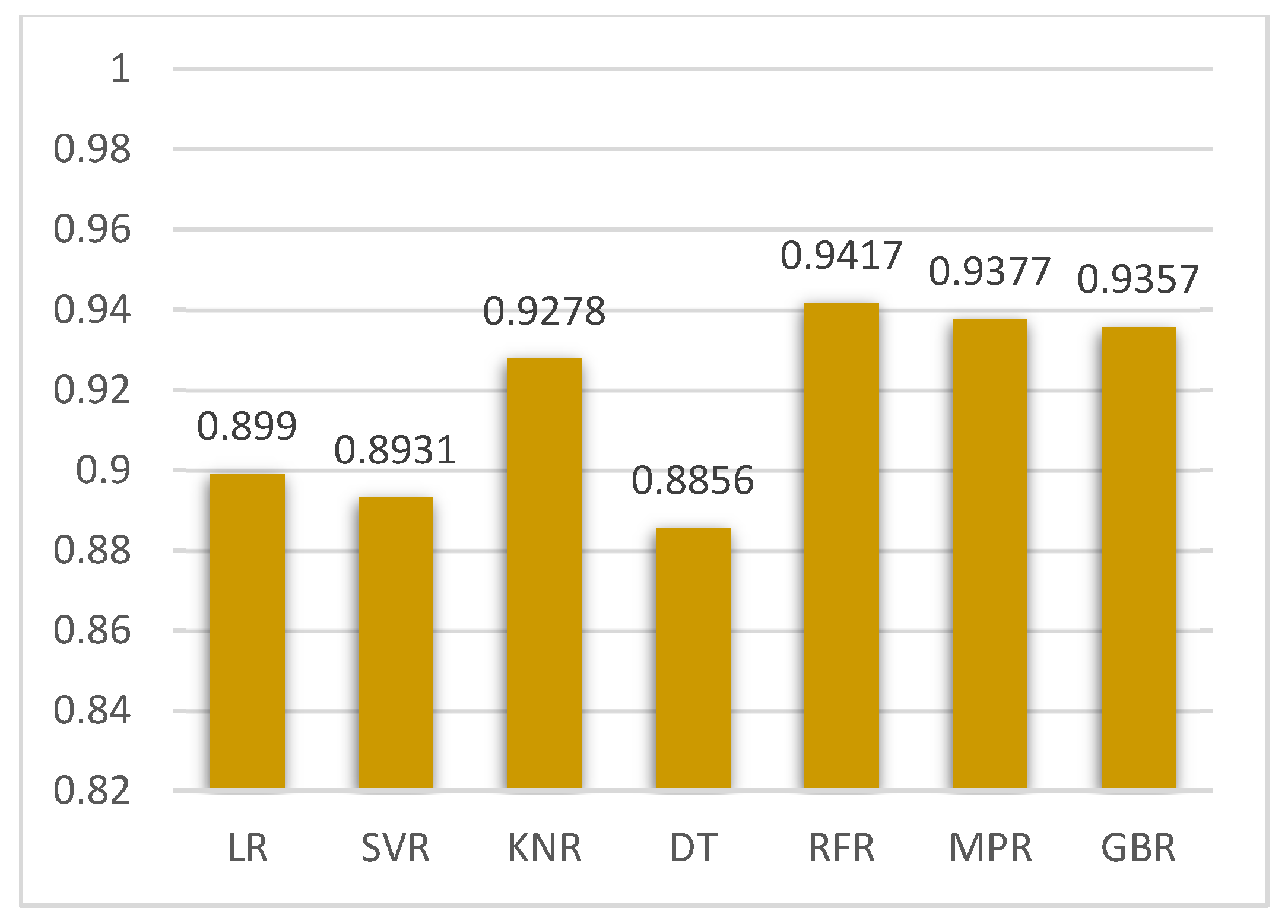
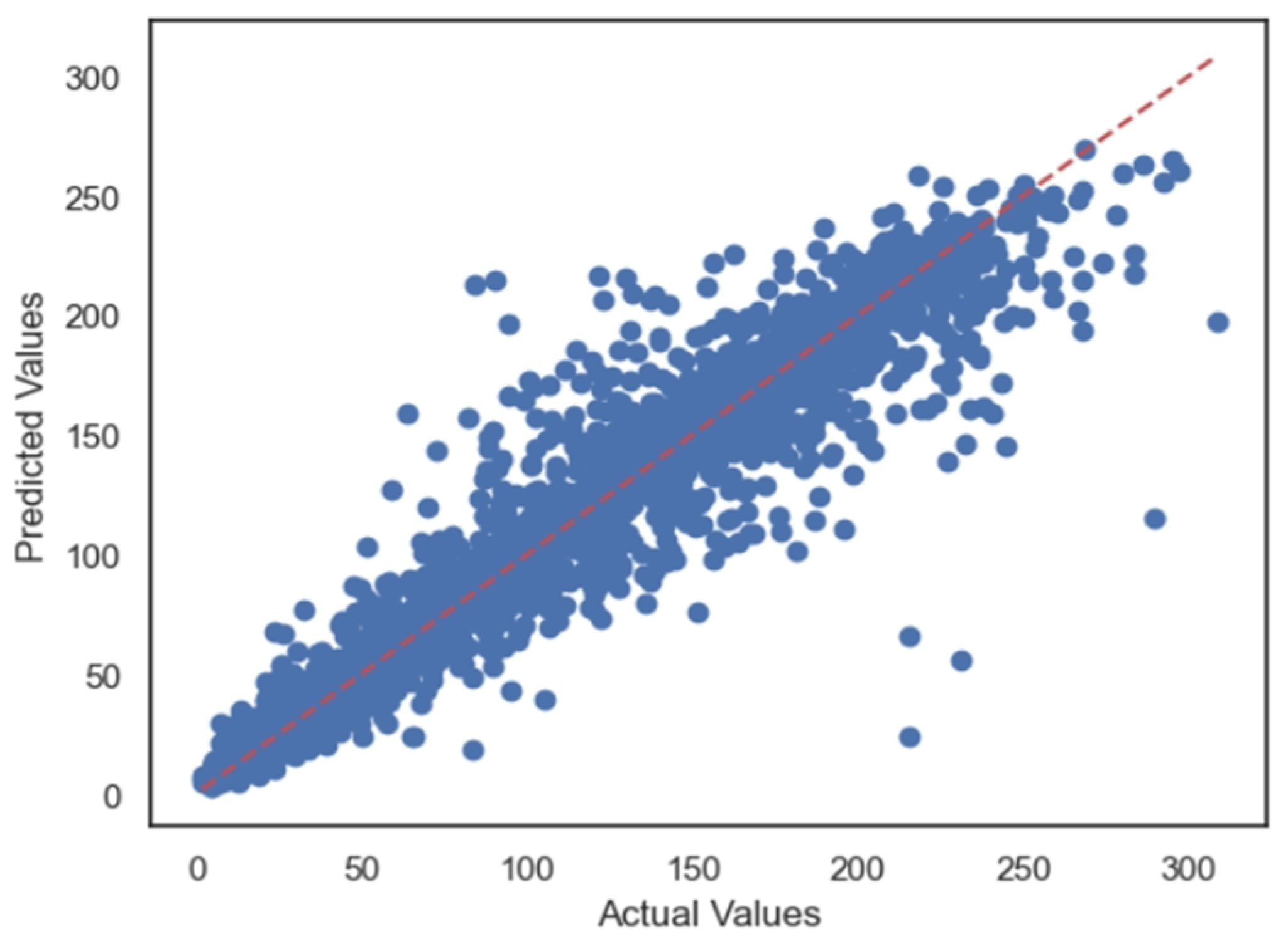
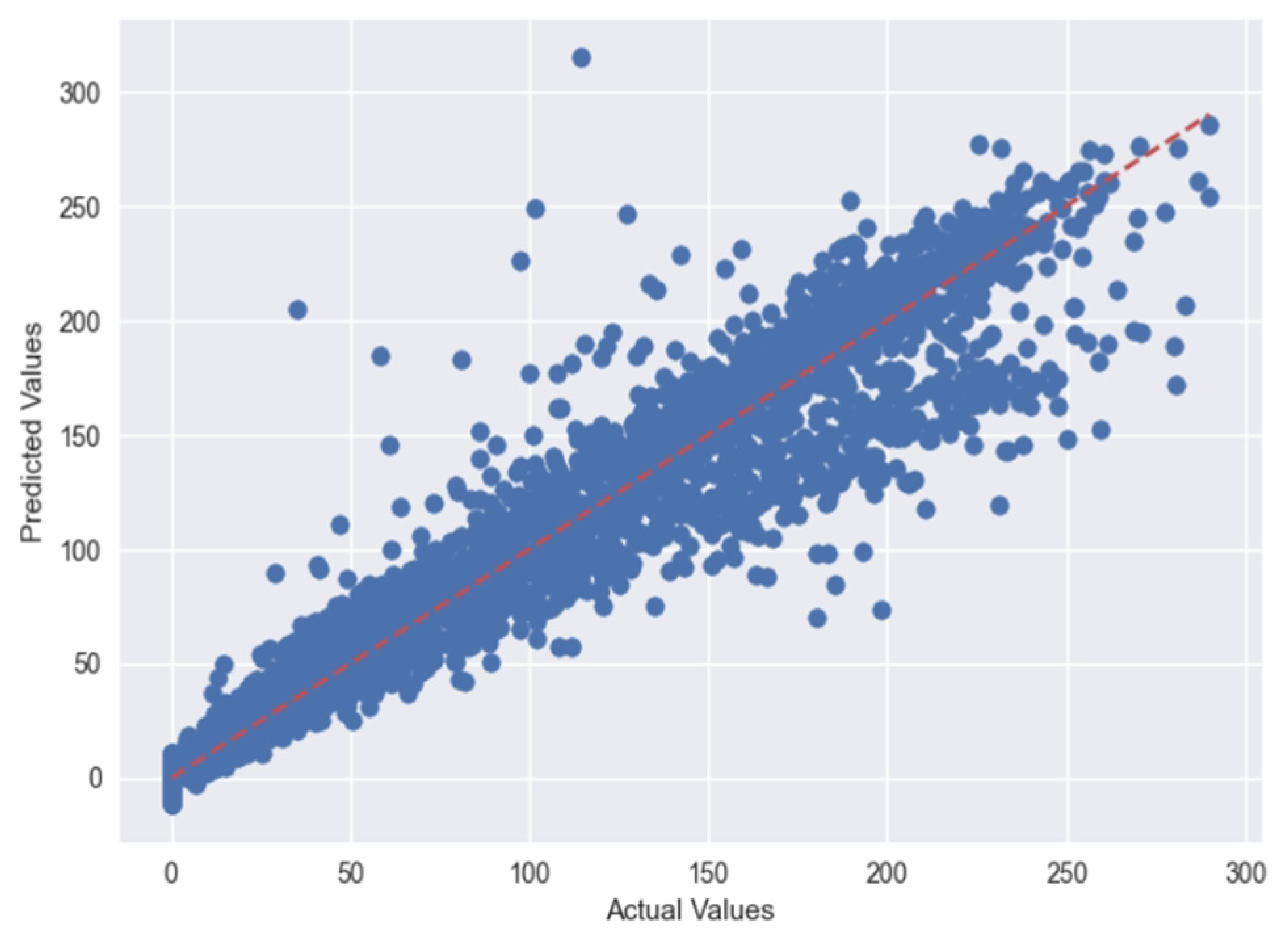
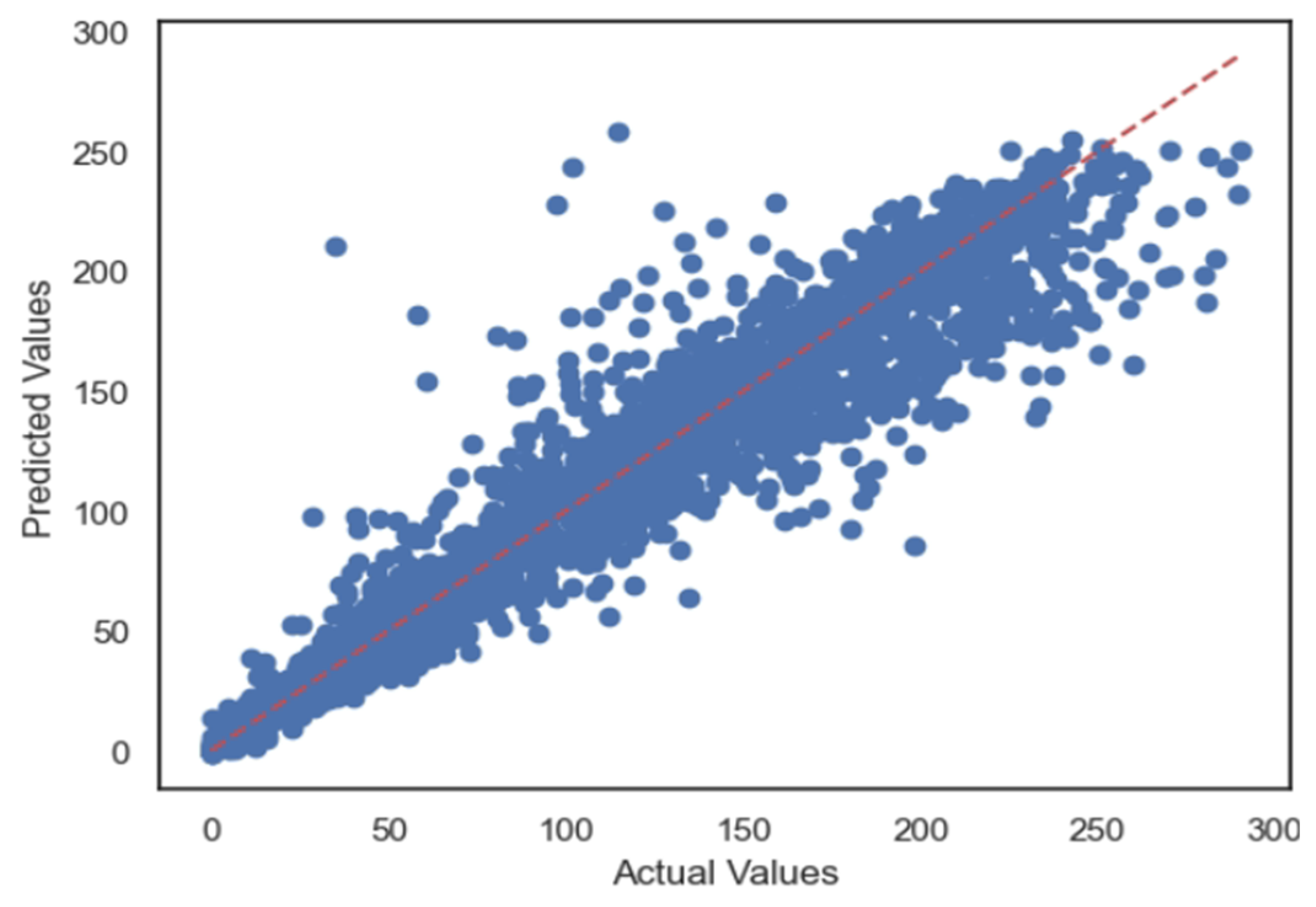
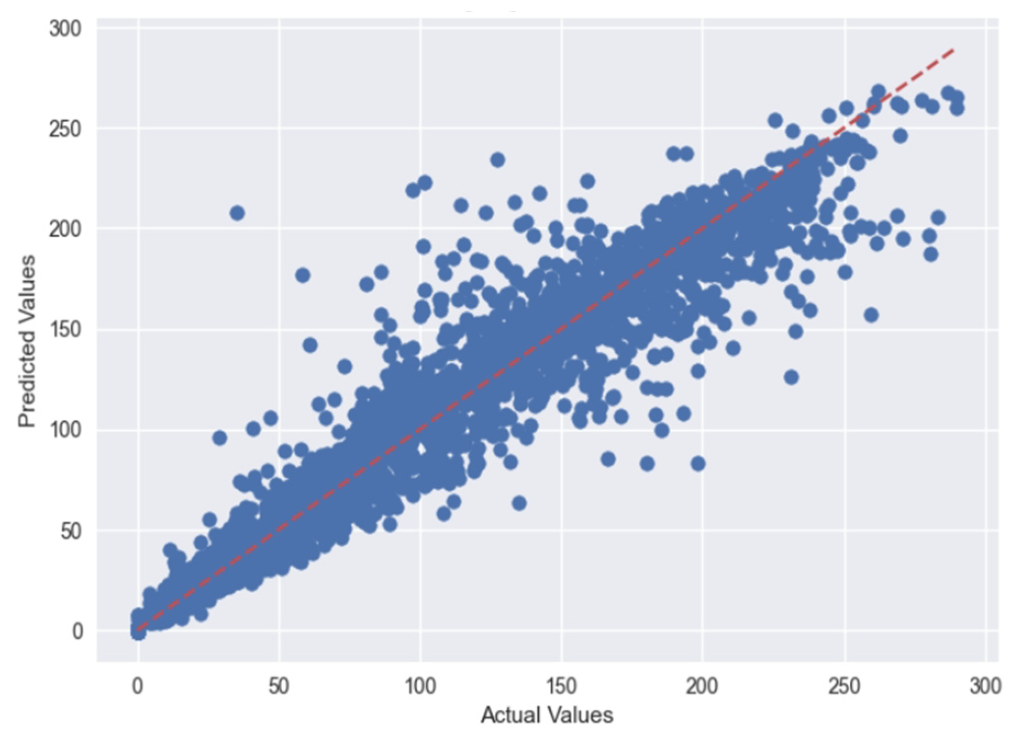
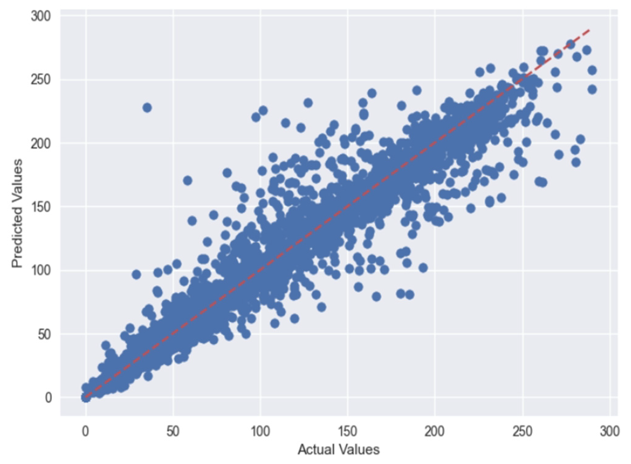
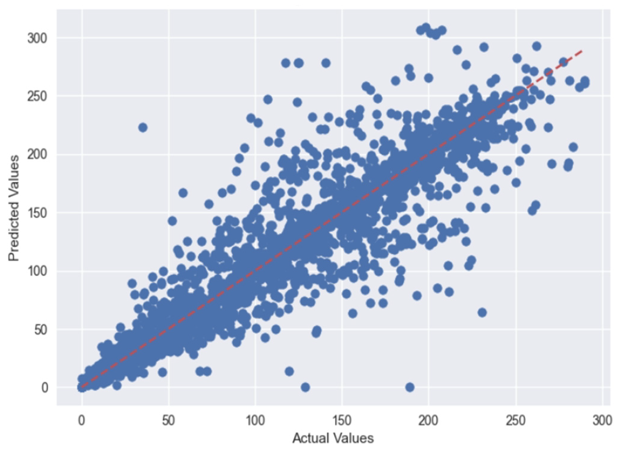
Figure 8 depicts the actual vs. predicted plots using LR. Figure 9 depicts the actual vs. predicted plots using SVR for Case 1. In a regression problem, the actual vs predicted plot visually assesses model performance. The red dotted diagonal line signifies perfect predictions, with blue points ideally aligning closely. Scattered points deviating from this line indicate model inaccuracies, highlighting potential performance issues. A clustered alignment around the diagonal line signifies robust model performance.

Figure 8.
Actual and predicted plots using LR.
Figure 8.
Actual and predicted plots using LR.
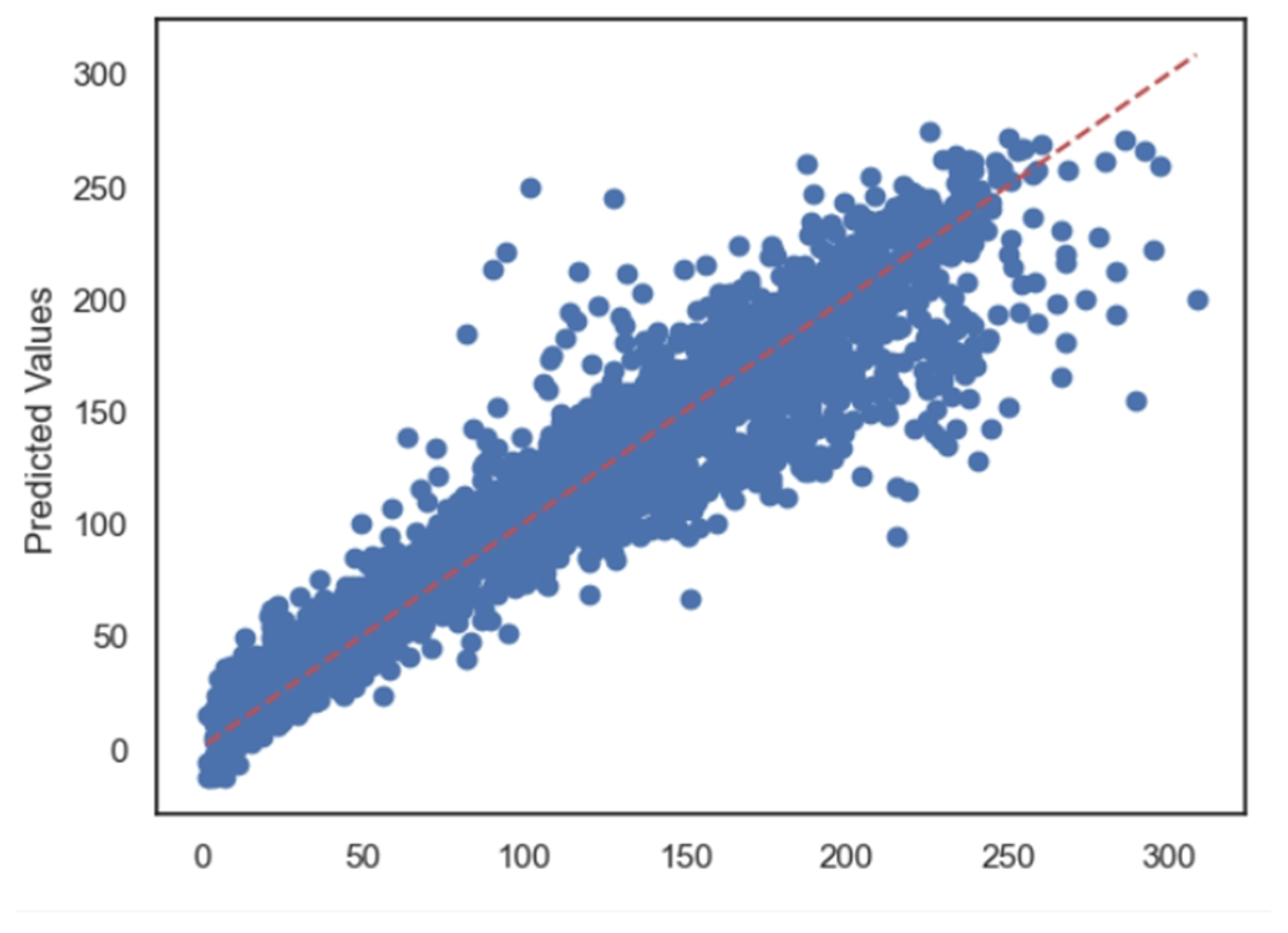

Figure 9.
Actual and predicted plots using SVR.
Figure 9.
Actual and predicted plots using SVR.
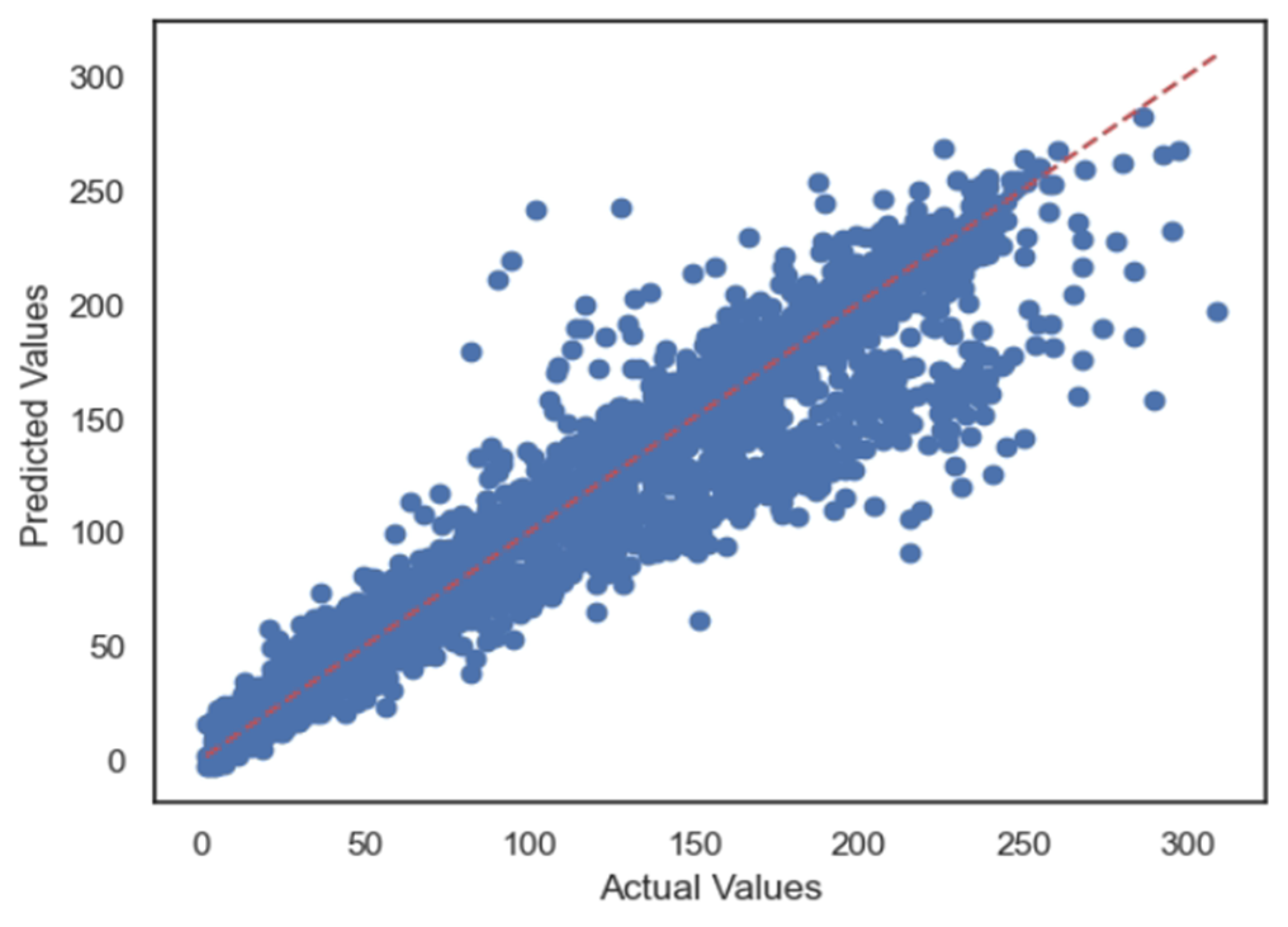
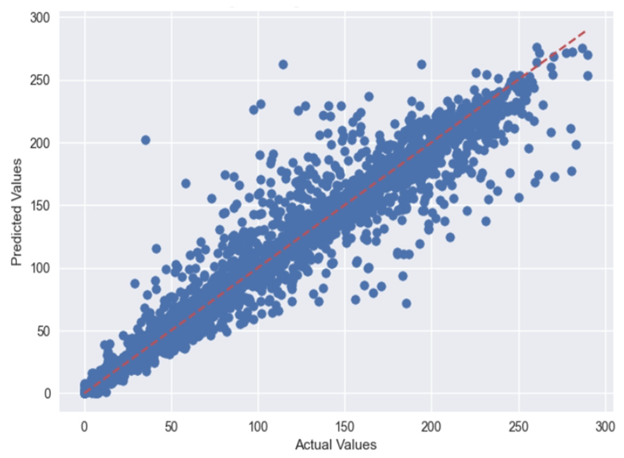
Figure 10 depicts the actual vs. predicted plots using the MLP regressor, and Figure 11 depicts the actual vs. predicted plots using GBR for Case 1.

Figure 10.
Actual and predicted plots using MLP.
Figure 10.
Actual and predicted plots using MLP.
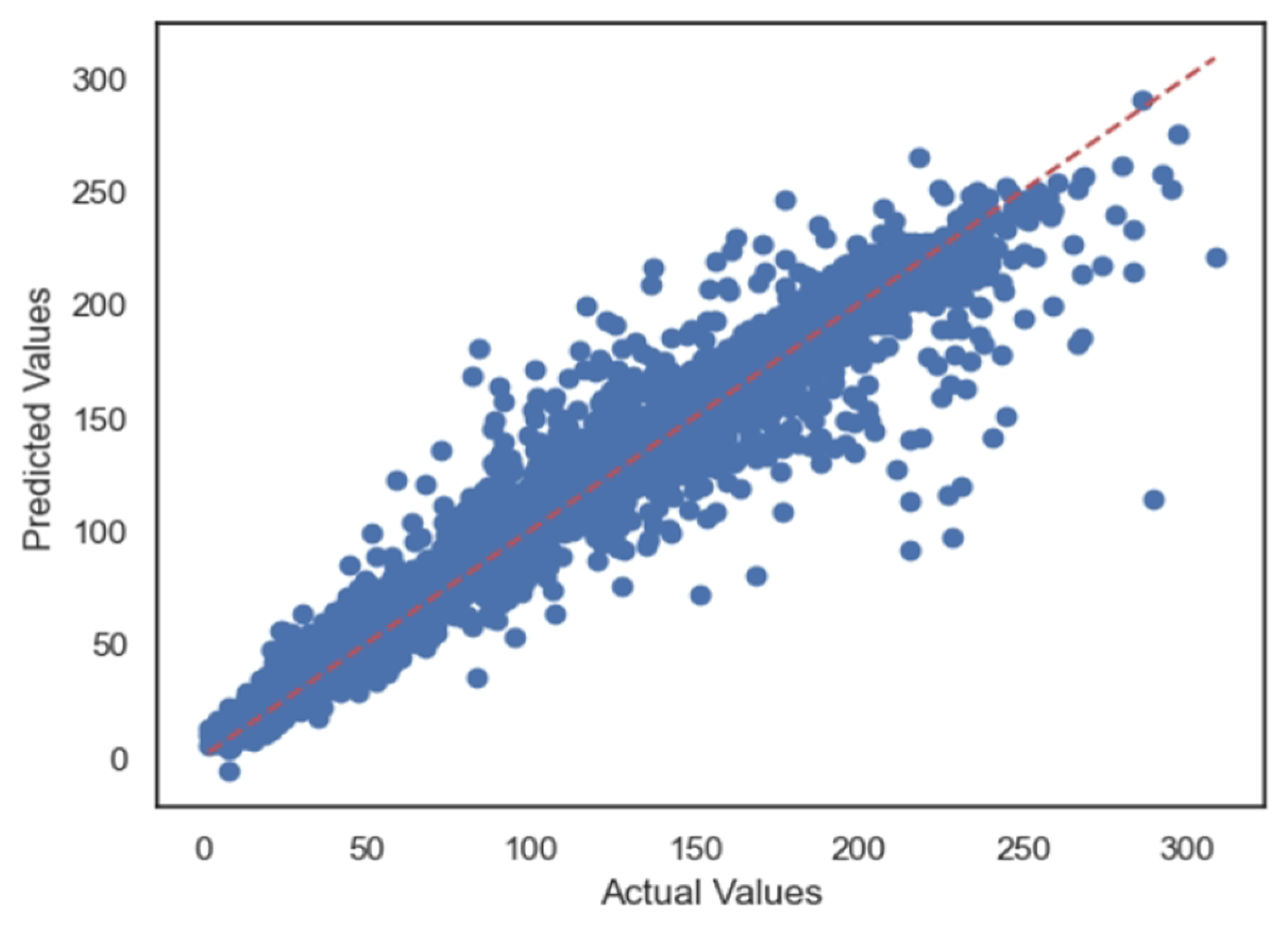
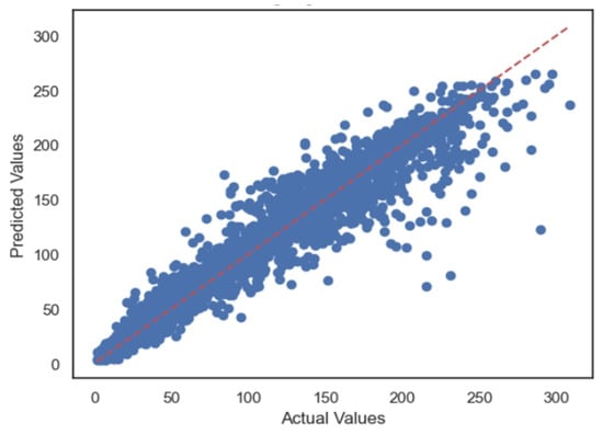
Figure 11.
Actual and predicted plots using GBR.
Figure 11.
Actual and predicted plots using GBR.

Figure 12 depicts the actual vs. predicted plots using RFR, and Figure 13 depicts the actual vs. predicted plots using DTR for Case 1.
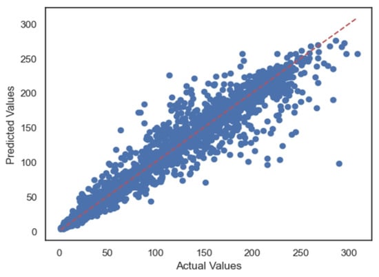
Figure 12.
Actual and predicted plots using RFR.
Figure 12.
Actual and predicted plots using RFR.


Figure 13.
Actual and predicted plots using DTR.
Figure 13.
Actual and predicted plots using DTR.
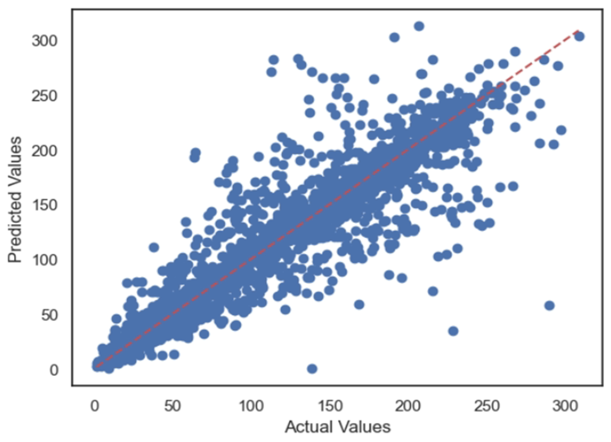
Figure 14 depicts the actual vs. predicted plots using KNR for Case 1.

Figure 14.
Actual and predicted plots using KNR.
Figure 14.
Actual and predicted plots using KNR.
5.2. Case 2:—Data Frame without Wind (Km/h) and PR% Features
Dropping rows from the dataset with NaN values in the PR% column, the row count of the dataset remains 14,220 from 25,656. To improve the performance of regression models, PR% with maximum NaN values and wind (Km/h) with a weak correlation with the power feature are dropped. The regression matrices are presented in Table 4.
Table 4.
MAE, MSE, RMSE, and R2 error outcomes in Case 2.
The efficacy and performance of the various ML regression models are presented in the form of MAE, MSE, RMSE, and R2 scores. Figure 15 of the article depicts the MAE scores obtained from various regression methods. The vertical axis represents the numeric values ranging from 0 to 18, and the values of MAE obtained using each regressor model are presented in the plot.
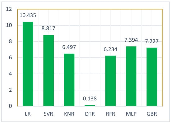
Figure 15.
MAE score plots of Case 2.
In contrast, Figure 16 depicts the MSE scores obtained from various regression methods. The vertical axis represents the numeric values ranging from 0 to 700, and the values of MSE obtained using each regressor model are presented in the plot.
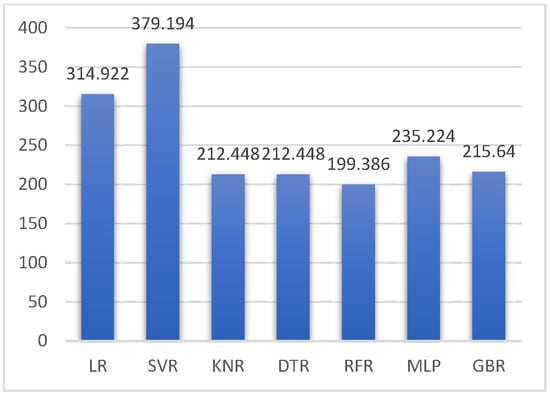
Figure 16.
MSE score plots of Case 2.
Similarly, Figure 17 depicts the RMSE scores obtained using various regression methods. The vertical axis represents the numeric values ranging from 0 to 30, and the values of RMSE obtained using each regressor model are presented in the plot.
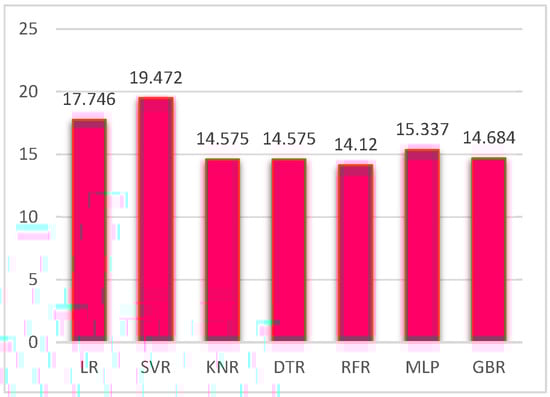
Figure 17.
RMSE score plots of Case 2.
Figure 18 illustrates the R2 values acquired from numerous regression approaches. The vertical axis indicates the numeric values ranging from 0.82 to 1.0, and the values of R2 obtained using each regressor model are shown in the plot.
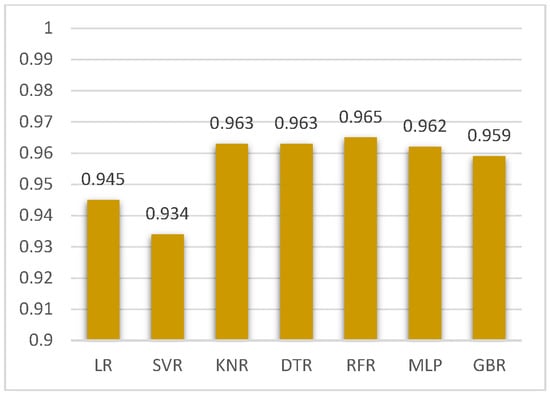
Figure 18.
R2 score plots of Case 2.
Figure 19 depicts the actual vs. predicted plots using LR; Figure 20 depicts the actual vs. predicted plots using SVR for Case 2.
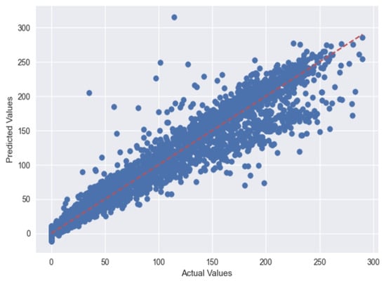
Figure 19.
Actual and predicted plots using LR in Case 2.
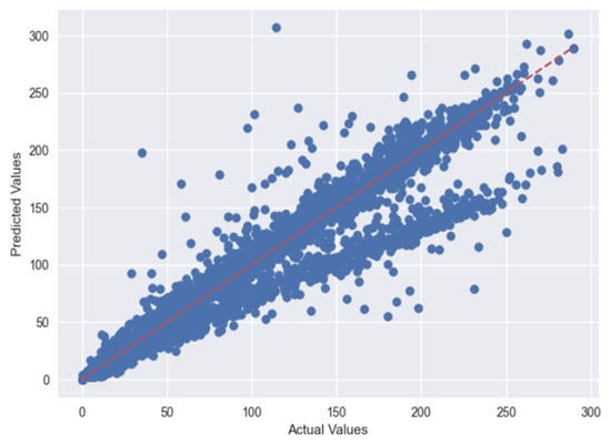
Figure 20.
Actual and predicted plots using SVR in Case 2.
Figure 21 depicts the actual vs. predicted plots using MLP, and Figure 22 depicts the actual vs. predicted plots using GBR for Case 2.

Figure 21.
Actual and predicted plots using MLP in Case 2.

Figure 22.
Actual and predicted plots using GBR in Case 2.
Figure 23 depicts the actual vs. predicted plots using RFR, and Figure 24 depicts the actual vs. predicted plots using DTR for Case 2.
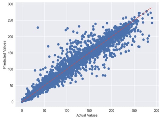
Figure 23.
Actual and predicted plots using RFR in Case 2.

Figure 24.
Actual and predicted plots using DTR in Case 2.
Figure 25 depicts the actual vs. predicted plots using LR for Case 2.
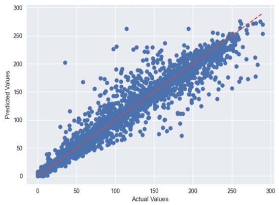
Figure 25.
Actual and predicted plots using KNR in Case 2.
6. Discussion
This section highlights a comparison of existing state-of-the-art regression modelling for PV power prediction using the R2 regression metric in Table 5.
Table 5.
Comparison analysis of various research articles vs. proposed methodology.
Compared to the cited research articles in Table 5, the proposed model has outperformed various regression methodologies in PV power prediction. However, the novelty of the model is determined by the portability of the best-performing regression method. The proposed model has harnessed 0.9650 of R2 value and uses a novel preprocessing strategy and steps. The feature engineering step in the proposed model used co-relation values to extract important features from the dataset.
7. Conclusions
This study demonstrates the propensity of the regression models to forecast PV power generation in PV systems. The Sharda PV dataset offers a variety of properties that have helped the proposed model significantly understand the correlation between these variables, which are significant in a majority of PV datasets used in research. The model’s efficacy and accuracy point to it becoming a crucial component in how enterprises develop and operate AI-powered PV grid systems. Given the opportunity for extra parameters in the dataset for model training, the proposed model could achieve higher success rates in addition to metrological properties. It is concluded that the proposed model can be useful for future research and serves as a foundation for improving PV power predictions. Numerous studies have examined the impact and participation of different deep learning models and ensemble approaches, and the findings have been encouraging. The authors intend to use deep learning methods and ensemble methods in future to develop and improve the model and its efficiency. Using the proposed model for datasets with a wide variety of feature vectors is also possible in the future.
Author Contributions
Methodology, N.U.I.; Software, N.U.I.; Investigation, B.U.D.A. and S.A.K.; Resources, S.L.; Data curation, S.L. and S.H.N.; Writing—original draft, B.U.D.A. and S.A.K.; Writing—review & editing, S.H.N.; Supervision, H.F. All authors have read and agreed to the published version of the manuscript.
Funding
This research received no external funding.
Data Availability Statement
The data presented in this study are available on request from the corresponding author.
Acknowledgments
Authors acknowledge Sharda University for the dataset.
Conflicts of Interest
The authors declare no conflict of interest.
References
- Kuzlu, M.; Cali, U.; Sharma, V.; Güler, Ö. Gaining insight into solar photovoltaic power generation forecasting utilizing explainable artificial intelligence tools. IEEE Access 2020, 8, 187814–187823. [Google Scholar] [CrossRef]
- Behera, M.K.; Majumder, I.; Nayak, N. Solar photovoltaic power forecasting using optimized modified extreme learning machine technique. Eng. Sci. Technol. Int. J. 2018, 21, 428–438. [Google Scholar] [CrossRef]
- Yang, H.-T.; Huang, C.-M.; Huang, Y.-C.; Pai, Y.-S. A weather-based hybrid method for 1-day ahead hourly forecasting of solar power output. IEEE Trans. Sustain. Energy 2014, 5, 917–926. [Google Scholar] [CrossRef]
- Zhou, H.; Rao, M.; Chuang, K.T. Artificial intelligence approach to energy management and control in the HVAC process: An evaluation, development and discussion. Dev. Chem. Eng. Miner. Process. 1993, 1, 42–51. [Google Scholar] [CrossRef]
- De Benedetti, M.; Leonardi, F.; Messina, F.; Santoro, C.; Vasilakos, A. Anomaly detection and predictive maintenance for photovoltaic systems. Neurocomputing 2018, 310, 59–68. [Google Scholar] [CrossRef]
- Elsaraiti, M.; Merabet, A. A comparative analysis of the arima and lstm predictive models and their effectiveness for predicting wind speed. Energies 2021, 14, 6782. [Google Scholar] [CrossRef]
- Lee, S.; Nengroo, S.H.; Jin, H.; Doh, Y.; Lee, C.; Heo, T.; Har, D. Anomaly detection of smart metering system for power management with battery storage system/electric vehicle. ETRI J. 2023, 45, 650–665. [Google Scholar] [CrossRef]
- Etxegarai, G.; López, A.; Aginako, N.; Rodríguez, F. An analysis of different deep learning neural networks for intra-hour solar irradiation forecasting to compute solar photovoltaic generators’ energy production. Energy Sustain. Dev. 2022, 68, 1–17. [Google Scholar] [CrossRef]
- Javanmard, M.E.; Ghaderi, S. A hybrid model with applying machine learning algorithms and optimization model to forecast greenhouse gas emissions with energy market data. Sustain. Cities Soc. 2022, 82, 103886. [Google Scholar] [CrossRef]
- Shedbalkar, K.H.; More, D. Bayesian Regression for Solar Power Forecasting. In Proceedings of the 2022 2nd International Conference on Artificial Intelligence and Signal Processing (AISP), Vijayawada, India, 12–14 February 2022; IEEE: Piscataway, NJ, USA, 2022; pp. 1–4. [Google Scholar]
- Nengroo, S.H.; Kamran, M.A.; Ali, M.U.; Kim, D.-H.; Kim, M.-S.; Hussain, A.; Kim, H.J. Dual battery storage system: An optimized strategy for the utilization of renewable photovoltaic energy in the United Kingdom. Electronics 2018, 7, 177. [Google Scholar] [CrossRef]
- Dash, P.; Majumder, I.; Nayak, N.; Bisoi, R. Point and interval solar power forecasting using hybrid empirical wavelet transform and robust wavelet kernel ridge regression. Nat. Resour. Res. 2020, 29, 2813–2841. [Google Scholar] [CrossRef]
- Nengroo, S.H.; Lee, S.; Jin, H.; Har, D. Optimal Scheduling of Energy Storage for Power System with Capability of Sensing Short-Term Future solar Power Production. In Proceedings of the 2021 11th International Conference on Power and Energy Systems (ICPES), Shanghai, China, 18–20 December 2021; IEEE: Piscataway, NJ, USA, 2021; pp. 172–177. [Google Scholar]
- Alfadda, A.; Adhikari, R.; Kuzlu, M.; Rahman, S. Hour-ahead solar power forecasting using SVR based approach. In Proceedings of the 2017 IEEE Power & Energy Society Innovative Smart Grid Technologies Conference (ISGT), Washington, DC, USA, 23–26 April 2017; IEEE: Piscataway, NJ, USA, 2017; pp. 1–5. [Google Scholar]
- Persson, C.; Bacher, P.; Shiga, T.; Madsen, H. Multi-site solar power forecasting using gradient boosted regression trees. Sol. Energy 2017, 150, 423–436. [Google Scholar] [CrossRef]
- Abuella, M.; Chowdhury, B. Solar power forecasting using support vector regression. arXiv 2017, arXiv:1703.09851. [Google Scholar]
- Huang, J.; Perry, M. A semi-empirical approach using gradient boosting and k-nearest neighbors regression for GEFCom2014 probabilistic solar power forecasting. Int. J. Forecast. 2016, 32, 1081–1086. [Google Scholar] [CrossRef]
- Lin, K.-P.; Pai, P.-F. Solar power output forecasting using evolutionary seasonal decomposition least-square support vector regression. J. Clean. Prod. 2016, 134, 456–462. [Google Scholar] [CrossRef]
- Bacher, P.; Madsen, H.; Nielsen, H.A. Online short-term solar power forecasting. Sol. Energy 2009, 83, 1772–1783. [Google Scholar] [CrossRef]
- Nengroo, S.H.; Jin, H.; Kim, I.; Har, D. Special Issue on Future Intelligent Transportation System (ITS) for Tomorrow and Beyond. Appl. Sci. 2022, 12, 5994. [Google Scholar] [CrossRef]
- Jin, H.; Nengroo, S.H.; Kim, I.; Har, D. Special issue on advanced wireless sensor networks for emerging applications. Appl. Sci. 2022, 12, 7315. [Google Scholar] [CrossRef]
- Al-Qahtani, F.H.; Crone, S.F. Multivariate k-nearest neighbour regression for time series data—A novel algorithm for forecasting UK electricity demand. In Proceedings of the 2013 International Joint Conference on Neural Networks (IJCNN), Dallas, TX, USA, 4–9 August 2013; IEEE: Piscataway, NJ, USA, 2013; pp. 1–8. [Google Scholar]
- El hadj Youssef, W.; Abdelli, A.; Kharroubi, F.; Dridi, F.; Khriji, L.; Ahshan, R.; Machhout, M.; Nengroo, S.H.; Lee, S. A Secure Chaos-Based Lightweight Cryptosystem for the Internet of Things. IEEE Access 2023, 11, 123279–123294. [Google Scholar] [CrossRef]
- Jin, H.; Nengroo, S.H.; Lee, S.; Har, D. Power Management of Microgrid Integrated with Electric Vehicles in Residential Parking Station. In Proceedings of the 2021 10th International Conference on Renewable Energy Research and Application (ICRERA), Istanbul, Turkey, 26–29 September 2021; IEEE: Piscataway, NJ, USA, 2021; pp. 65–70. [Google Scholar]
- Lee, S.; Nengroo, S.H.; Jin, H.; Doh, Y.; Lee, C.; Heo, T.; Har, D. Power management in smart residential building with deep learning model for occupancy detection by usage pattern of electric appliances. In Proceedings of the 2023 5th International Electronics Communication Conference, Osaka City, Japan, 21–23 July 2023; pp. 84–92. [Google Scholar]
- Lee, S.; Jin, H.; Nengroo, S.H.; Doh, Y.; Lee, C.; Heo, T.; Har, D. Smart Metering System Capable of Anomaly Detection by Bi-directional LSTM Autoencoder. In Proceedings of the 2022 IEEE International Conference on Consumer Electronics (ICCE), Las Vegas, NV, USA, 7–9 January 2022; IEEE: Piscataway, NJ, USA, 2022; pp. 1–6. [Google Scholar]
- Lee, S.; Nengroo, S.H.; Jung, Y.; Kim, S.; Kwon, S.; Shin, Y.; Lee, J.; Doh, Y.; Heo, T.; Har, D. Factory Energy Management by Steam Energy Cluster Modeling in Paper-Making. In Proceedings of the 2023 11th International Conference on Smart Grid (icSmartGrid), Paris, France, 4–7 June 2023; IEEE: Piscataway, NJ, USA, 2023; pp. 1–5. [Google Scholar]
- Rifat, M.S.H.; Niloy, M.A.; Rizvi, M.F.; Ahmed, A.; Ahshan, R.; Nengroo, S.H.; Lee, S. Application of Binary Slime Mould Algorithm for Solving Unit Commitment Problem. IEEE Access 2023, 11, 45279–45300. [Google Scholar] [CrossRef]
- Lai-Dang, Q.-V.; Nengroo, S.H.; Jin, H. Learning dense features for point cloud registration using a graph attention network. Appl. Sci. 2022, 12, 7023. [Google Scholar] [CrossRef]
- Munawar, U.; Wang, Z. A framework of using machine learning approaches for short-term solar power forecasting. J. Electr. Eng. Technol. 2020, 15, 561–569. [Google Scholar] [CrossRef]
- Mishra, M.; Dash, P.B.; Nayak, J.; Naik, B.; Swain, S.K. Deep learning and wavelet transform integrated approach for short-term solar power prediction. Measurement 2020, 166, 108250. [Google Scholar] [CrossRef]
- Aslam, M.; Lee, S.-J.; Khang, S.-H.; Hong, S. Two-stage attention over LSTM with Bayesian optimization for day-ahead solar power forecasting. IEEE Access 2021, 9, 107387–107398. [Google Scholar] [CrossRef]


Disclaimer/Publisher’s Note: The statements, opinions and data contained in all publications are solely those of the individual author(s) and contributor(s) and not of MDPI and/or the editor(s). MDPI and/or the editor(s) disclaim responsibility for any injury to people or property resulting from any ideas, methods, instructions or products referred to in the content. |
© 2024 by the authors. Licensee MDPI, Basel, Switzerland. This article is an open access article distributed under the terms and conditions of the Creative Commons Attribution (CC BY) license (https://creativecommons.org/licenses/by/4.0/).