Charging Behavior Portrait of Electric Vehicle Users Based on Fuzzy C-Means Clustering Algorithm

Abstract

The rapid increase in electric vehicles (EVs) has led to a continuous expansion of electric vehicle (EV) charging stations, imposing significant load pressures on the power grid. Implementing orderly charging scheduling for EVs can mitigate the impact of large-scale charging on the power grid. However, the charging behavior of EVs significantly impacts the efficiency of orderly charging plans. By integrating user portrait technology and conducting research on optimized scheduling for EV charging, EV users can be accurately classified to meet the diverse needs of various user groups. This study establishes a user portrait model suitable for park areas, providing user group classification based on the user response potential for scheduling optimization. First, the FCM and feature aggregation methods are utilized to classify the quantities of features of EV users, obtaining user portrait classes. Second, based on these classes, a user portrait inventory for each EV is derived. Third, based on the priority of user response potential, this study presents a method for calculating the feature data of different user groups. The individual data information and priorities from the user portrait model are inputted into the EV-optimized scheduling model. The optimization focuses on the user charging cost and load fluctuation, with the non-dominated sorting genetic algorithm II utilized to obtain the solutions. The results demonstrate that the proposed strategy effectively addresses the matching issue between the EV user response potential and optimal scheduling modes without compromising the normal use of EVs by users. This classification approach facilitates the easier acceptance of scheduling tasks by participating users, leading to optimized outcomes that better meet practical requirements.

1. Introduction

With the proposal of the national “dual carbon” goal, EVs have obvious advantages in protecting the environment, saving energy, reducing emissions, and alleviating human dependence on petroleum [1,2]. As of 2021, the global ownership of EVs has reached 16.5 million, and the projected global market share of EVs is expected to reach USD 190 billion by 2030 [3,4]. The increasing scale of the charging load of EVs will significantly affect the operation and planning of regional power grids [5,6]. The assessment of the impacts of EV charging scheduling has received extensive attention recently [7]. Under a reasonable scheduling strategy, EVs can not only help the power grid relieve the pressure on the power grid during unordered charging [8,9,10,11] but also provide auxiliary services such as frequency modulation and backup power for the power grid [12,13]. However, the complex charging behaviors of EV users directly impact the practical implementation of charging scheduling [14,15]. The accurate analysis of the charging behavior of EVs has become the primary issue in EV charging scheduling [16].

Plenty of researchers have conducted extensive research on the charging behavior of EVs, with a specific emphasis on strategies to reduce the overall charging costs for users and mitigate the potential impacts on grid stability caused by high-demand charging. The charging behaviors of EVs have differentiated time, urgency, and flexibility [17]. Ref. [18] summarized that the charging behaviors of EVs are related to the user’s thoughts, preferences, and habits. Ref. [19] made a statistical analysis on the charging behavior of EV users in Ireland, revealing that the charging patterns of EV owners are time-dependent and unaffected by location. Ref. [20] found that private EV owners choose night charging with lower electricity prices, which should mean lower overnight electricity prices. The findings in [21] indicated that factors such as charging time, the distance to a charging station, charging cost, remaining battery energy, and maximum battery rechargeable energy all play a significant role in influencing drivers’ charging decisions. Different charging behaviors have a significant impact on the load curve of the power grid [22]. Predictions for the orderly charging load of EVs have been made through the analysis of EV charging behavior [23]. Based on the analysis of EV charging behavior, the burden on the electrical grid can be alleviated by shifting charging times [24]. Actually, several scholars have made great efforts to classify EV users. Chen J. et al. [25] studied models of EV charging stations, which were categorized into five types based on travel purposes: home, work, shopping, social interaction, and others.

The analysis of EV users either employs a user group approach or focuses on typical vehicles. The research referenced in [26,27,28] concentrates on the behavior of EV user groups, overlooking the differences between each EV. Research on each EV focuses on the behavioral features of typical vehicles and obtains the charging behavior of each EV user through probability analysis [29], traffic travel law simulation [30,31,32], and big data processing [33,34].

Compared to research on user group behavior, the study strategy of focusing on typical vehicles proves to be more accurate when analyzing EV behavior [35]. However, research from the perspective of typical vehicles alone overlooks the diversity of group vehicle behaviors and fails to accommodate the vast scale of EV users, presenting limitations.

The analysis of EV charging behavior mostly adopts the clustering method [36]. Clustering is one of the basic algorithms of unsupervised machine learning. Common clustering methods include K-means clustering, the density-based spatial clustering of applications with noise (DBSCAN), fuzzy c-means clustering (FCM), the Gaussian mixture model (GMM), etc. In cluster analysis, FCM is a soft clustering algorithm. It can automatically divide clusters based on the distance between sample points and is more flexible than other clustering methods [37,38]. The study clusters the charging start time, charging end time, charging time, and charging amount, classifies EV users, and predicts EV charging behavior [39,40].

In the field of power load analysis, user portrait technology accurately portrays the features of power consumers using labeled indicators related to energy consumption and electricity usage [41]. By integrating user portrait technology with research on optimizing EV charging schedules, EV users can be effectively classified to meet the varying needs of different user groups. This study proposes a combined approach that integrates both group and individual user behavior analysis, which can satisfy the behavior analysis of large-scale vehicle users while also enhancing the accuracy of user group behavior analysis. This study establishes a user response portrait model and proposes a precise portrait strategy for EVs in a campus setting. This strategy provides user group classification based on response potential for scheduling optimization, making it easier for participating users to accept scheduling tasks, resulting in more realistic optimization outcomes. The research content is shown in Figure 1 below. The main contributions of this study are as follows:

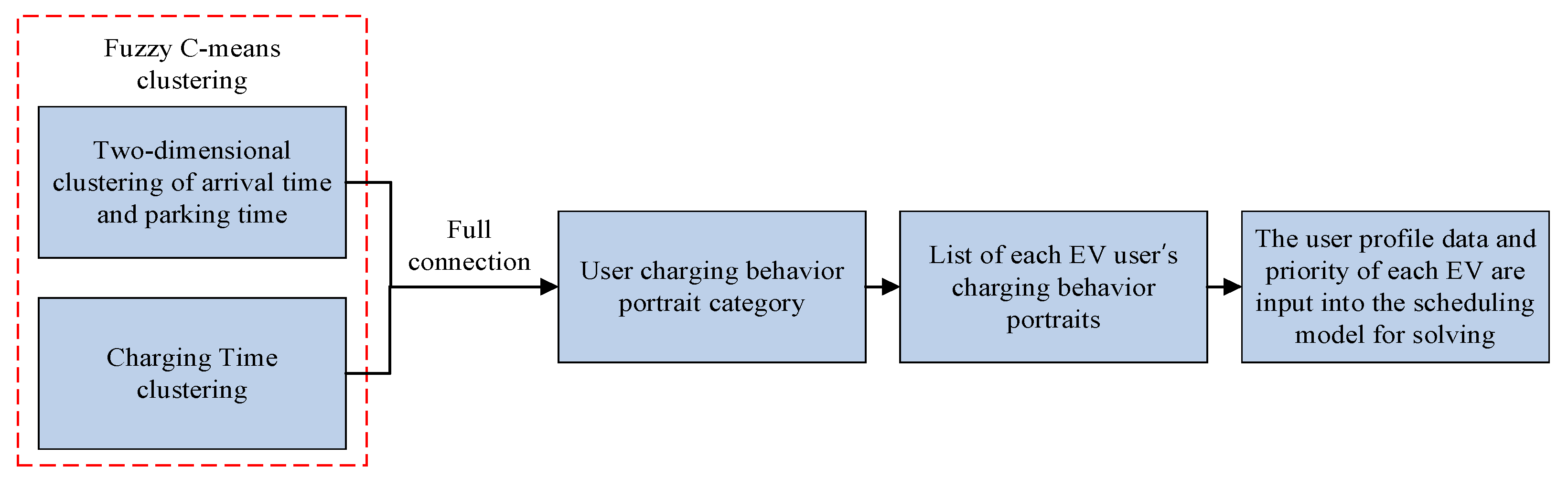
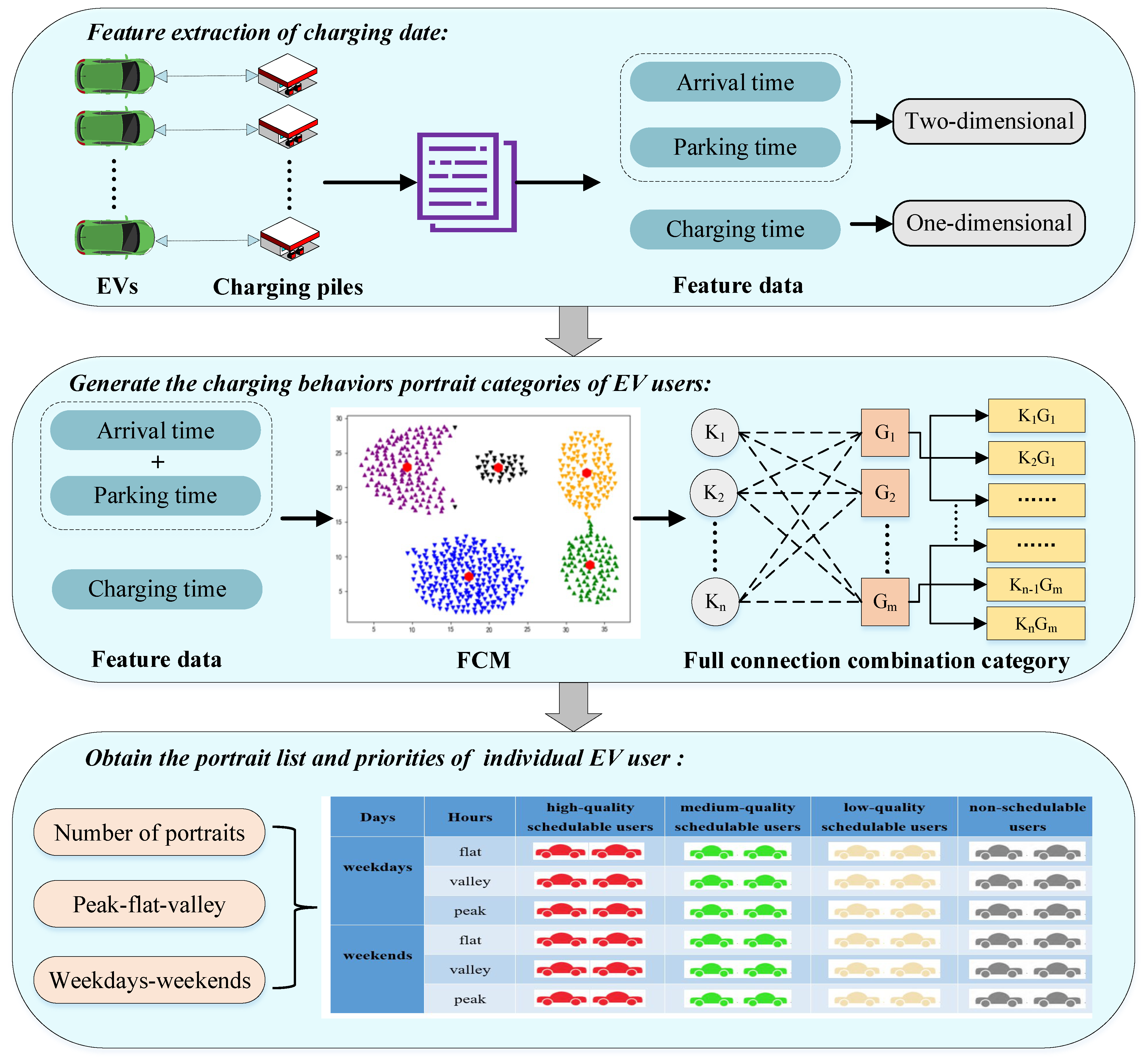
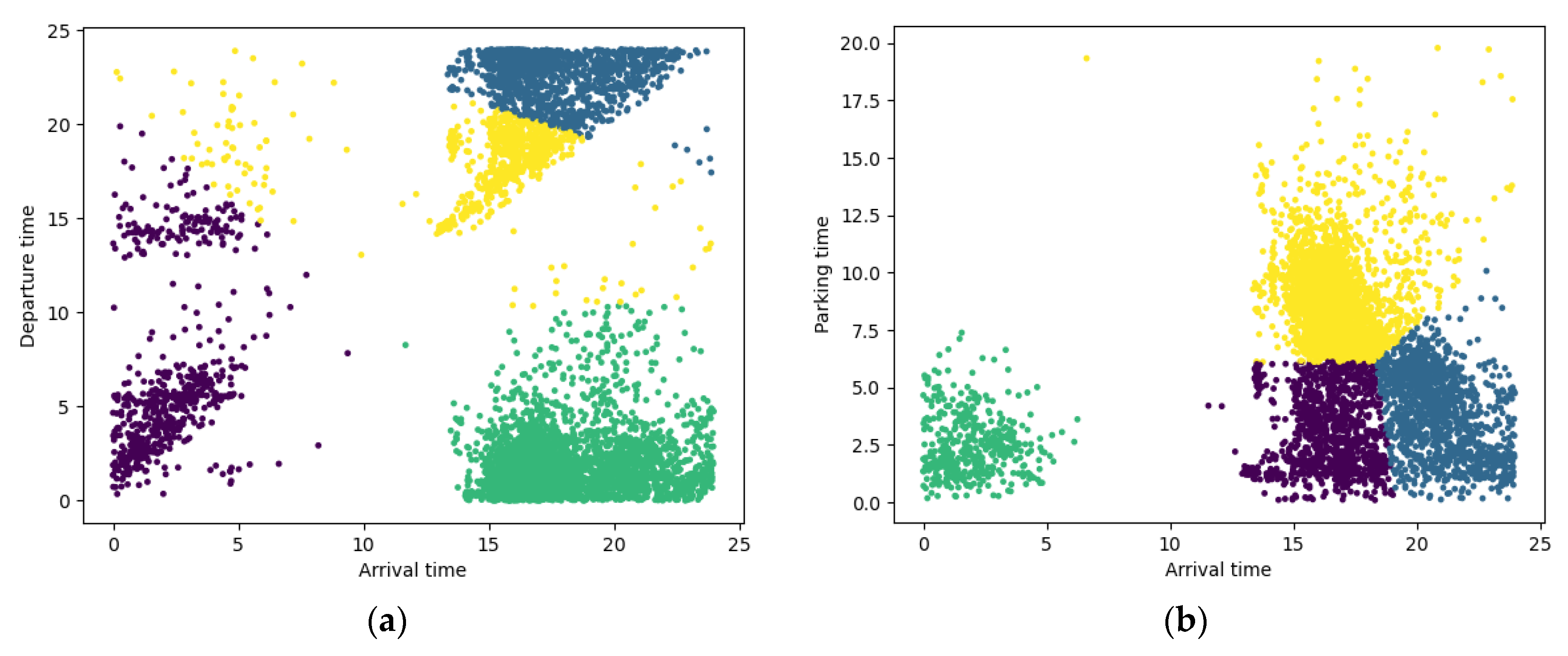
• The charging behavior portraits of EV users are characterized using FCM. The two-dimensional clustering results of the arrival time and parking time of EVs and the clustering results of charging time are aggregated by features, and the charging portrait categories of EVs in the park are obtained.
• This study introduces a portrait model that combines group portrait categories with individual EVs. Each portrait category corresponds to a different range of features, and the charging data of each EV may include one or several portrait categories, thus generating a list of user portraits for each EV. Based on the duration of schedulable time associated with each portrait category, EV users are categorized into four types: high-quality schedulable users, medium-quality schedulable users, low-quality schedulable users, and irregular users.
• In order to enhance the accuracy of the user portraits, this study conducted further statistics based on the charging patterns on weekdays and weekends. The statistics were categorized into weekday charging, weekend charging, and weekday–weekend charging for each EV. This study introduces the classification of dispatchable EVs and their priorities during the peak/flat/valley load periods.
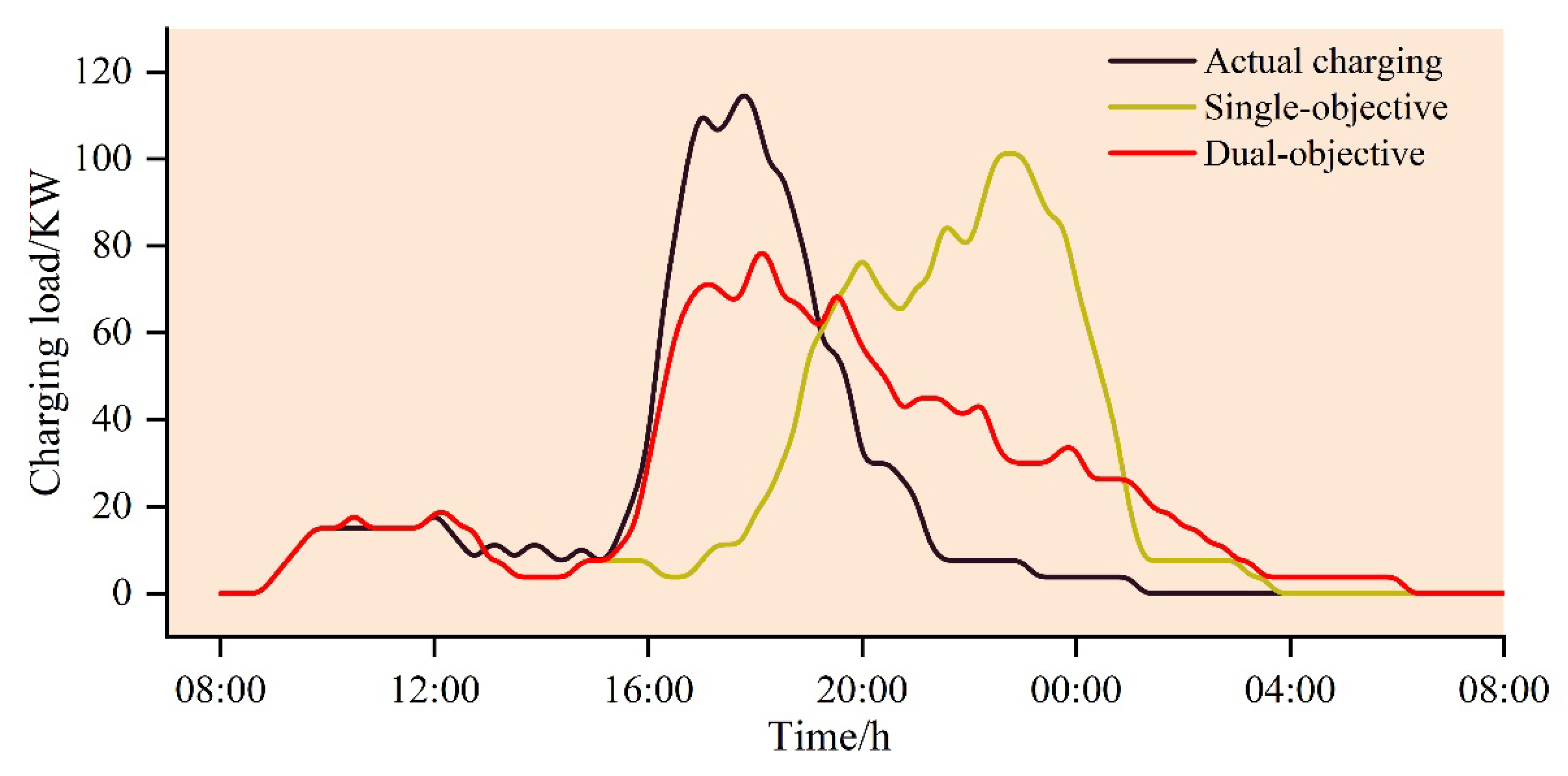
• Based on the priority of user response potential, this study presents a method for calculating the feature data of different user groups. The data are inputted into the EV scheduling optimization model for computation and solution, resulting in optimized scheduling outcomes for each user group. While ensuring user satisfaction is not compromised, the diverse needs of the power grid can be met based on the priority of user groups. This study validates the feasibility of certain user group portraits through three charging scheduling scenarios. The experimental results demonstrate that when considering the charging cost of EV users as a single objective function, the charging cost is reduced by 47.42% compared to unstructured charging. When both the charging cost and load fluctuation of EV users are considered as dual objective functions, the charging cost of EV users and the load fluctuation of the charging station are reduced, respectively, by 41.76% and 31.07%.

2. Research Framework and Methodology

The research framework of this study is shown in Figure 2. The first part of the research framework—the EV users’ charging behavior portrait categories—was obtained. The charging behaviors of multiple EV users in the park were reasonably classified by clustering and feature aggregation, and the charging portrait categories of EVs in the park were obtained. The second part of the research framework, the charging behavior of each EV, can be characterized using one or multiple user profile categories. The orderly scheduling priority of EVs is determined by considering both the proportion of each EV portrait and the scheduling time. Moreover, the dispatchable EVs and their priority during the peak/flat/valley load periods are further studied. The specific steps in the two parts are shown in Figure 2.

2.1. EV Users’ Charging Behavior Portrait Categories

2.1.1. Collection and Preprocessing of Data

The necessary dataset for this research needed to be collected. Data preprocessing involves various tasks such as data cleaning, calculation, transformation, and normalization. Data cleaning included the removal and filling of missing data. Some EV charging data are sparse and considered irregular users; thus, these were excluded from the clustering analysis. Abnormal information in the original dataset was corrected accordingly. In case of missing features, either elimination or filling with the median value was performed for the data points. Incorrect data, such as the charging time exceeding the stay time, were removed from consideration. Data calculation entails deriving useful information through computations. Data transformation involves converting different types of data into numerical formats recognizable by clustering algorithms. Lastly, data normalization was conducted to scale the original data within the range 0–1 in order to eliminate impacts of amplitude.

2.1.2. Feature Extraction

When analyzing user arrival and departure times, it is crucial to account for instances where EV users do not arrive and depart within the same calendar day. The parking time of each EV is calculated based on arrival time, departure time, and the date difference between the two time points, regardless of overnight stays or visits spanning multiple days.

$$T_p=T_d-T_a+24\ast D_{date}$$

(1)

where $T_p$ is the parking time, $T_a$ is the arrival time, and $T_d$ is the departure time. $D_{date}$ is the difference in dates between the arrival time and the departure time. In this study, the arrival time, parking time, and charging time from the data were chosen as feature parameters.

2.1.3. FCM Clustering

The FCM algorithm is a clustering algorithm. In this algorithm, the degree of affiliation of each sample point with all class centroids is determined through the optimization of a specific objective function. Upon the acquisition of these membership values, they were utilized as a foundational criterion for the categorization of the sample dataset.

The difference between the FCM algorithm and traditional clustering algorithms is that the former changes the “either/or” phenomenon of clustering, and an object can belong to multiple categories in different degrees. Compared with K-means hard clustering, FCM clustering provides more flexible clustering results. Considering the complexity of EV users’ charging behaviors, FCM clustering was used in this study to analyze EV charging behaviors. The three key parameters of FCM clustering are the number of clusters, the center of mass of clusters, and the cluster corresponding to data points.

(1)

Objective function.

The objective function of clustering is essentially the sum (the sum of squares of errors) of the Euclidean distances from various points to various classes. FCM clustering is the calculation of the minimum value of the objective function under the condition that the membership constraint function is met. The process of clustering solves the minimum objective function and reduces the error value of the objective function through repeated iterative operations. When the objective function converges, the final clustering result is obtained, and the formulas of the objective function are as follows:

$$J_m={\displaystyle \sum _{i=1}^N{\displaystyle \sum _{j=1}^C{u}_{ij}^m}}{\Vert x_i-v_j\Vert }^2, 1\le m<\infty$$

(2)

Constraints:

$${\displaystyle \sum _{j=1}^C{u}_{ij}=1,\forall i=1,2\cdots N}$$

(3)

where $m$ is the fuzzy index, $N$ is the data volume, and $c$ is the number of clustering centers. $v_j$ represents the $j$-th center, $x_i$ represents the $i$-th sample, and $u_{ij}$ represents the membership degree of the sample $x_i$ to the clustering center. $v_j$.$\parallel \ast \parallel$ can be any measure that represents the similarity (distance) of data, and the most common one is the Euclidean norm.

(2)

The membership degree matrix $u_{ij}$ and cluster center $v_j$.

The membership matrix represents the degree to which each sample point belongs to each class. For a single sample, $x_i$, its membership to each cluster adds up to 1. The objective function is related to Euclidean distance. When the objective function reaches the minimum, the Euclidean distance is the shortest. This guarantees the clustering principle of the highest intra-group similarity and the lowest inter-group similarity. The formulas of the membership degree matrix and cluster center are as follows:

$$u_{ij}=\frac{1}{{\displaystyle \sum _{k=1}^C{\left(\frac{\parallel x_i-v_j\parallel }{\parallel x_i-v_k\parallel }\right)}^{\frac{2}{m-1}}}}$$

(4)

$$v_j=\frac{{\displaystyle \sum _{i=1}^N{u}_{ij}^m{x}_i}}{{\displaystyle \sum _{i=1}^n{u}_{ij}^m}}$$

(5)

where $u_{ij}$ and $v_j$ are interrelated. FCM clustering is a process of iteratively calculating membership $u_{ij}$ and cluster centers $v_j$ until they reach an optimal level.

(3)

The termination condition of iteration.

$$\max \left|u_{ij}^{t+1}-u_{ij}^t\right|<\epsilon$$

(6)

where $t$ is the number of iteration steps, and $\epsilon$ is the error threshold. $u_{ij}$ and $v_j$ are updated in the iteration until the maximum change in the membership degree before and after two iterations does not exceed the error threshold, and, at this time, the comparative optimal (local optimal or global optimal) state is reached. The process eventually converges to the local minimum or saddle point of the target $J_m$.

The detailed description of each step is described as follows:

Step 1.

Initialize the matrix determined by the membership function $U_0$ (initialized between random values [0, 1]) while satisfying the constraints of Formula (3).

Step 2.

Calculate the central value of the cluster $v_j$ according to Formula (5).

Step 3.

Calculate the new membership matrix $u_{ij}$ according to Formula (4).

Step 4.

Calculate the change in the objective function this time and the last time according to Formula (2). If the change is less than a certain threshold, then stop the algorithm; otherwise, go to Step 2.

This clustering process is divided into the following two parts:

The arrival time and parking time of EVs are clustered as $K_1,K_2\dots \dots K_n$ using the two-dimensional FCM algorithm.

$$f_{FCM}(T_a \& T_p)=\{K_1,K_2,\dots ,K_n\}$$

(7)

The one-dimensional fuzzy FCM algorithm is used to calculate the charging time of EVs to obtain $G_1,G_2\cdots \cdots G_m$.

$$f_{FCM}(T_c)=\{G_1,G_2,\dots ,G_m\}$$

(8)

where $f_{FCM}(T_a \& T_p)$ is the result of arrival time and parking time clustering, and $f_{FCM}(T_c)$ is the result of charging time length clustering.

2.1.4. Feature Aggregation

When opting for three-dimensional clustering, it becomes challenging to distinguish between categories. Based on literature references and data analysis, two-dimensional clustering involving arrival time and parking time is selected, and the results are combined with the clustering of charging time for feature aggregation.

Feature aggregation refers to clustering different feature quantities or feature vectors separately and then combining all clustering results into new categories. Through feature aggregation, related features in the original data can be combined to reduce the dimensionality and complexity of the data, extracting more representative and informative features. This helps improve the performance and accuracy of models as well as uncover deeper relationships between data. Feature aggregation is commonly used in feature engineering and data preprocessing processes.

According to the clustering results $K_1,K_2\dots \dots K_n$ of the arrival time and parking time of EV users and the clustering results $G_1,G_2\dots \dots G_n$ of the charging time of EV users, feature aggregation was conducted to form portrait categories to describe the charging behavior of EVs, as shown in Figure 3.

By using feature aggregation and eliminating irrelevant categories, all user portrait categories could be identified accurately. By analyzing the relationship between parking time and charging time, the feasible scheduling time for each portrait category could be established, usually by deducting the charging time from the parking time. A longer scheduling time indicates higher optimal scheduling behavior within the user’s charging portrait category.

2.2. Analysis of the Charging Behavior of Each EV

(1)

EV charging on weekdays and weekends.

Different users have different patterns of charging behavior on weekdays and weekends, which can be generally divided into three categories: charging on weekdays, charging on weekends, and charging on both weekdays and weekends.

(2)

The charging behavior portrait of each EV.

Strictly, the complexity of each EV user’s charging behavior cannot be fully represented by individual portraits. Each portrait category corresponds to different feature quantities (selected arrival time, parking time, and charging time), and the charging data information of each EV user matches one or more portrait categories. The list of the user charging behavior portrait also differs. Here, the charging behavior portrait of each EV is listed according to the user’s charging behavior portrait category.

(3)

Determine the rules of the user’s charging behavior portrait.

The list of EV users’ charging behavior portraits for each EV may contain multiple portraits. However, if there are too many portraits in the process, there will be many difficulties in the subsequent study of EV users’ charging behavior usage. In order to guarantee the accuracy of the portraits of EV users’ charging behaviors and provide a fast method for orderly charging scheduling, one or several portraits of EV users’ charging behaviors with a large proportion are selected as the final portraits of this EV. Based on this, if the set portrait rules are met, all EVs are divided into regular charging EV users; otherwise, they are divided into irregular charging EV users.

Based on the clustering process, criteria for assessing the priority of EV users have been established as follows:

• If the percentage of any single portrait category data reaches between L and 100%, the user is classified as a high-quality user.
• If the combined percentage of any two portrait category data reaches between L and 100%, the user is classified as a medium-quality user.
• If the combined percentage of any three portrait category data reaches between L and 100%, the user is classified as a low-quality user.
• Users who do not fall into the above categories are classified as irregular users.

Based on these criteria, users were classified as high-quality, medium-quality, low-quality, or irregular users.

The response potential of different user groups affects the dispatch efficiency of the power grid. The response capability of high-quality users is higher than that of medium-quality users, and the response capability of medium-quality users is higher than that of low-quality users. When EVs are dispatched into the power grid, priority is given to users with higher priority levels, as the dispatch results are more likely to be accepted by users, avoiding impacting user satisfaction and travel usage. Irregular users cannot learn from vehicle user behavior and, thus, are not selected for dispatch.

3. Case Study

In order to test the effect of the model, the dataset selected for this study was ACN-Data, which is a public dataset used for EV charging research. The ACN-Data data were collected from two real-world adaptive charging network facilities in California. The adaptive charging network facility on the Caltech campus is in a parking lot and has 54 EVSEs (EV supply equipment or charging stations; EV power supply devices or parks) and a 50 kW DC fast charger. (All the experimental parts are executed using Python 3.9 on an Intel (R) Core (TM) i5-10500 CPU 3.10 GHz system with 16 GB RAM. Additionally, keras2.7 and sklearn0.0 post 12 are selected as the main deep learning framework for model training).

In this study, the data from one year (a total of 6555 pieces of data from 28 October 2018 to 28 October 2019) were used, and 53 vehicles with abundant charging data were selected to analyze users’ charging behaviors.

3.1. EV Users’ Charging Behavior Portrait Categories

3.1.1. Data Preprocessing

After the abnormal data were removed, 6283 pieces of data were available, including the charging data of 53 vehicles (charging pile number, vehicle number, arrival time, start time of charging, stop time of charging, departure time, etc.).

3.1.2. Feature Extraction

Considering that the arrival date and departure date may not be the same day, in order to avoid introducing errors in the results, the parking time was selected and obtained through calculation. In Figure 4a, the clustering results of arrival time and departure time exhibit clusters with close inter-cluster distances and relatively dispersed points within the clusters, indicating poor classification effectiveness. On the other hand, in Figure 4b, the clustering results of arrival time and parking time clearly delineate four distinct categories. Meanwhile, the charging time of EVs was selected by considering the difference in EV users’ charging power and battery capacity. 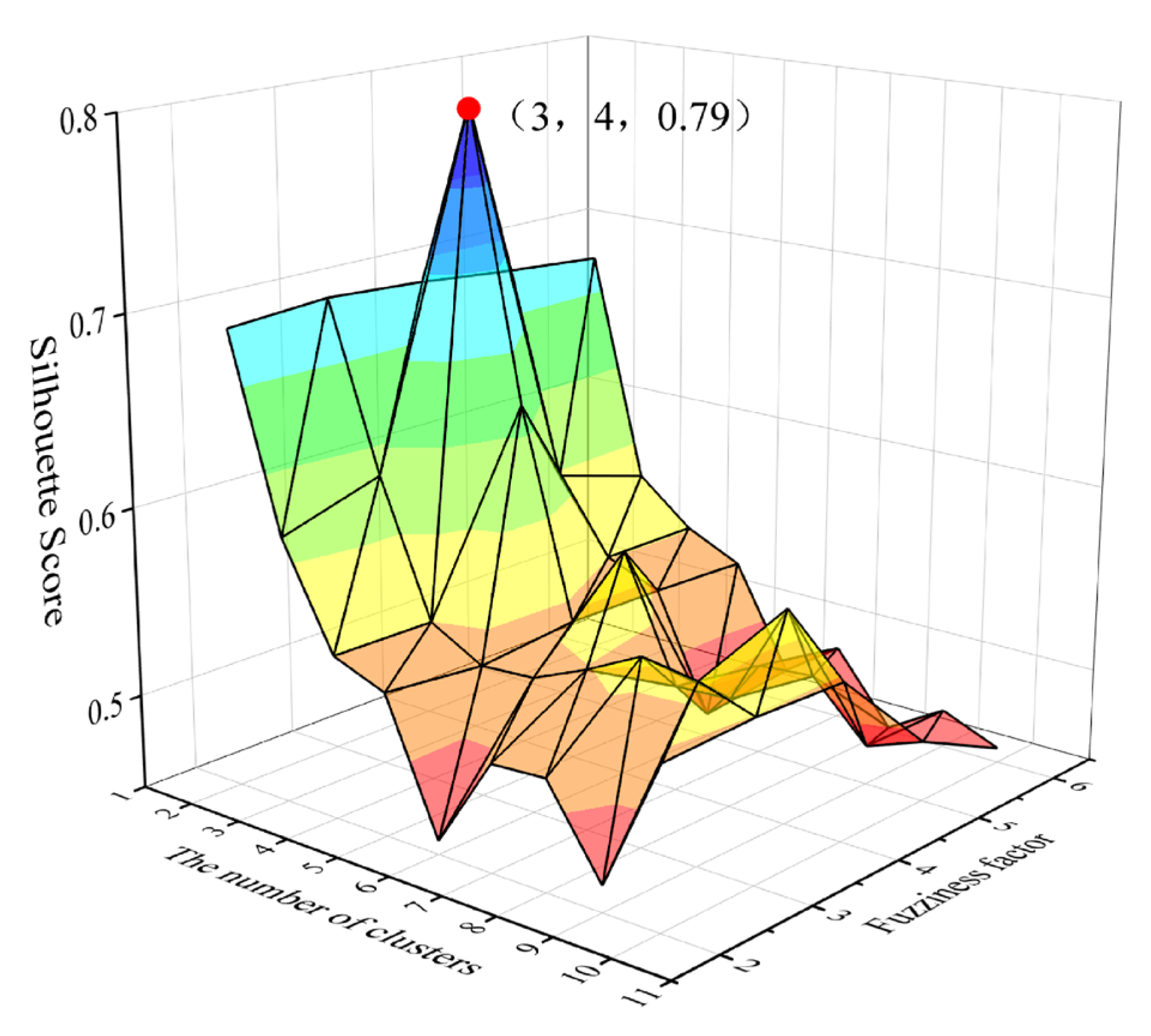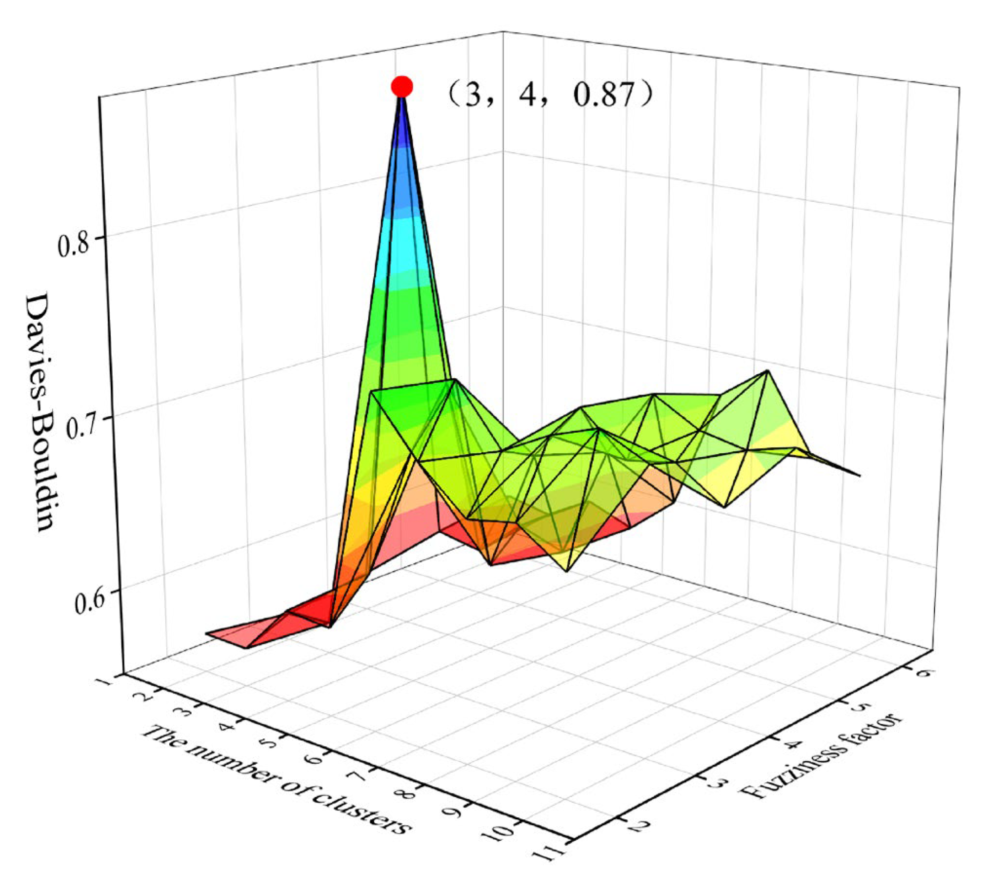The arrival time, parking time, and charging time of EV users at the charging pile were selected as the feature quantities with which to describe the charging behavior portrait of EV users and were converted into a digital format that could be used for clustering.

3.1.3. FCM Clustering

The silhouette score is one of the commonly used evaluation metrics for clustering, and the specific formula is shown below:

$$S=\frac{1}{n}{\displaystyle \sum _{i=1}^n\frac{b(x_i)-a(x_i)}{max\{b(x_i),a(x_i)\}}}$$

(9)

where $n$ represents the total number of data points in the cluster set, $x_i$ denotes the clustered data, $a\left(x_i\right)$ is the average distance between $x_i$ and the other points within the same cluster set, and $b\left(x_i\right)$ is the average distance between $x_i$ and the points in the other different cluster sets; the silhouette score ranges from −1 to 1, where a higher value indicates better clustering performance.

The Calinski–Harabaz score is also one of the commonly used metrics for measuring clustering effectiveness, with the specific formula as follows:

$$s\left(k\right)=\frac{tr(B_k)}{tr(W_k)}\frac{m-k}{k-1}$$

(10)

where $m$ represents the number of samples in the training set, $k$ denotes the number of clusters, $B_k$ is the covariance matrix between clusters, $W_k$ is the covariance matrix within clusters, and $tr(\cdot )$ denotes the trace of a matrix. A larger Calinski–Harabaz factor indicates better clustering effectiveness.

Firstly, two-dimensional FCM clustering was performed on arrival time and parking time. The parameters of the FCM clustering were optimized, including the number of clusters and the fuzziness factor. Figure 5 and

Table 1. The value of the silhouette score of the two-dimensional FCM under different numbers of clusters and different fuzziness factors.

	Fuzziness Factor	2	3	4	5	6
K
2		0.389443	0.395071	0.393793	0.392867	0.392487
3		0.532903	0.531693	0.529861	0.459066	0.234224
4		0.631191	0.382821	0.373935	0.367385	0.272961
5		0.410918	0.405724	0.398312	0.392735	0.195995
6		0.386903	0.344528	0.321615	0.312594	0.306506
7		0.372883	0.337231	0.353385	0.317599	0.142264
8		0.364074	0.337235	0.315556	0.306669	0.294148
9		0.358419	0.327525	0.277566	0.269329	0.171575
10		0.3556	0.330718	0.305587	0.283643	0.27148

display the silhouette score of the two-dimensional FCM under different numbers of clusters and different fuzziness factors. Figure 6 and

Table 2. The value of the Calinski–Harabaz score of the two-dimensional FCM under different numbers of clusters and different fuzziness factors.

	Fuzziness Factor	2	3	4	5	6
K
2		1.297386	1.308402	1.302959	1.29969	1.265925
3		1.348359	0.616996	0.618025	0.858865	0.616264
4		1.474923	0.85197	0.851415	0.845798	1.662239
5		1.119099	0.780511	0.796129	0.806442	0.763778
6		0.995778	0.861625	0.950117	0.9807	0.793255
7		1.155263	0.860409	0.963581	1.011551	0.838428
8		1.092277	0.876527	0.88891	1.016422	0.844842
9		1.210399	0.922233	1.061232	1.037081	0.884294
10		1.07599	0.936428	1.017053	1.057625	0.884567

display the Calinski–Harabaz score of the two-dimensional FCM under different numbers of clusters and different fuzziness factors.

From Figure 5 and Figure 6, it can be observed that when the silhouette score and fuzziness factor are set to 2 and 4, respectively, FCM achieves the best clustering results. According to the analysis of the results of multiple experiments, in order to achieve better classification results, the two-dimensional clustering of arrival time and parking time is divided into four categories, and the charging time is divided into three categories. The results are presented in Figure 4b.

For a more intuitive representation, the clustering results are shown in a normal distribution diagram (Figure 7).

Secondly, one-dimensional FCM clustering was conducted for EV charging time. Figure 8 and

Table 3. The value of the silhouette score of the one-dimensional FCM under different numbers of clusters and different fuzziness factors.

	Fuzziness Factor	2	3	4	5	6
K
2		0.691652	0.695154	0.691652	0.686091	0.681525
3		0.590455	0.607002	0.790455	0.576179	0.56041
4		0.536281	0.535715	0.636281	0.536453	0.536589
5		0.525425	0.520158	0.525425	0.524821	0.522881
6		0.457113	0.522049	0.571373	0.462612	0.468237
7		0.506349	0.534602	0.506349	0.498334	0.489293
8		0.508161	0.549598	0.508161	0.500806	0.451887
9		0.463691	0.54531	0.563691	0.470788	0.470259
10		0.533726	0.53577	0.533726	0.482042	0.457723

display the silhouette score of the one-dimensional FCM under different numbers of clusters and different fuzziness factors. Figure 9 and

Table 4. The value of the Calinski–Harabaz score of the one-dimensional FCM under different numbers of clusters and different fuzziness factors.

	Fuzziness Factor	2	3	4	5	6
K
2		0.57263	0.565634	0.57263	0.581957	0.588573
3		0.572094	0.568296	0.872094	0.577003	0.583342
4		0.602113	0.605636	0.702113	0.600107	0.599057
5		0.600321	0.682988	0.600321	0.590946	0.589008
6		0.737542	0.73023	0.672308	0.658926	0.612362
7		0.706368	0.696925	0.706368	0.699832	0.685206
8		0.682917	0.711881	0.682917	0.684912	0.705973
9		0.68834	0.722074	0.68834	0.679799	0.659787
10		0.670146	0.709694	0.670146	0.687916	0.655985

display the Calinski–Harabaz scores of the one-dimensional FCM under different numbers of clusters and different fuzziness factors.

From Figure 8 and Figure 9, it can be observed that when the silhouette score and fuzziness factor are set to 3 and 4, respectively, FCM achieves the best clustering results. Based on the difference in EV users’ electricity demand and charging power, the charging times of EVs were selected as the feature quantities for clustering analysis, and the multi-user’s charging time was divided into classes. Figure 10 shows the normal distribution of charging time.

3.1.4. Generate User Charging Behavior Profile Categories

Considering the complexity of the users’ charging behavior, according to the cluster of arrival times and parking times, as well as the cluster of charging times, a new cluster was generated by using feature aggregation to form the portrait category of the overall users’ charging behavior. According to the parameters mean value and variance that determine the normal distribution curve, this study takes each feature quantity for each cluster datum as the numerical range of this cluster, indicating that 68% of the data in this set fall within this numerical range.

According to the rationality of the value and the principle that parking time is longer than charging time, any unreasonable user portraits were removed, and nine categories were formed through reasonable combination. Then, graphs were generated for each category with a normal distribution, as shown in Figure 11.

3.1.5. Schedulable Time of User Charging Behavior Profile Category

The time that can be scheduled in the charging process can be obtained according to the portrait, and the value of parking time subtracted from the charging time is the scheduling time of each portrait type. The longer the scheduling time, the better the flexibility and schedulability of the scheduling of reasonable and orderly charging of EVs, and the better the portrait type of a user’s charging behavior.

Table 5. The scheduling time by user charging behavior profile category.

Portrait Category	K1G1	K1G2	K2G1	K2G2	K3G1	K3G2	K4G1	K4G2	K4G3
Scheduling duration	0:00–1:55	0:25–4:13	0:00–1:49	0:00–2:53	0:00–0:53	0:00–1:43	3:07–7:04	5:35–9:15	0:00–2:37
Data volume	338	964	283	833	101	371	821	1999	543
Arrival time	19:15–22:07	19:35–22:20	14:34–17:42	14:58–17:46	0:34–3:02	0:46–3:19	15:09–17:49	15:37–18:03	15:03–17:35

shows the scheduling time duration by user portrait category.

According to the time-sharing pricing of regional peak load in California, USA, the electricity consumption period can be divided into the valley period (23:00–8:00), peak period (12:00–19:00), and flat period. According to the peak–valley period and dispatching time of the power grid, in which the arrival time is located, the priority ranking of the categories of user charging behavior portraits is shown in

Table 6. Charging scheduling priority based on user charging behavior profile category.

Time of Arrival	User Behavior Portrait Prioritization
Valley period	K3G1, K3G2
Flat period	K1G1, K1G2
Peak period	K2G1, K2G2, K4G1, K4G2, K4G3

.

3.2. Each User’s Charging Behavior Analysis

3.2.1. User Charging Behavior Analysis Based on Weekdays and Weekends

According to EV users’ travel preferences on weekdays and weekends, the daily charging frequency can be roughly divided into three categories: charging on weekdays, charging on weekdays and weekends, and charging on weekends. A total of 53 vehicles were classified (below) according to the number of trips per day, as shown in

Table 7. Analysis of daily trips of EVs.

Weekday–Weekend Charging Categories	User ID
Weekdays	515, 558, 559, 560, 562, 620, 668, 676, 832, 1095, 1124, 1137, 1534, 1912, 1082, 567, 714, 69, 2170, 1126, 632, 2461, 850, 569, 1470, 858, 1104, 945, 1001, 1154, 1164, 1524, 431, 818, 712, 1099, 324, 1366, 1154
Weekdays and Weekends	1108, 777, 609, 1202, 1222, 754, 1135, 1083, 838, 891, 1161, 743, 1746, 1133
Weekends	248

.

3.2.2. User Charging Behavior Portrait of Each Car

Based on the complexity of EV users’ charging behaviors for each vehicle, this study describes the behaviors of a single vehicle and determines the charging behavior portraits of each EV user by using the proportion of nine categories. A vehicle cannot be completely represented by a user charging behavior portrait category. According to the criteria in the article, L is set to 70. In Appendix A, if the percentage of any single portrait category data reaches 70–100%, the user is classified as a high-quality schedulable user and marked in red. If the combined percentage of any two portrait category data reaches 70–100%, the user is classified as a medium-quality schedulable user and marked in green. If the combined percentage of any three portrait category data reaches 70–100%, the user is classified as a low-quality schedulable user and marked in blue. Users who do not fall into the above categories are classified as irregular users and are marked in purple.

3.3. EV Optimal Scheduling Model

Smart charging of EVs can help reduce user costs and grid fluctuations [42,43,44]. Smart charging involves establishing objective functions, constraints, and optimization plans. By combining methods to profile the charging behavior of EV users, we obtained feature data for each user, and these were input into the EV scheduling model. Based on user priority, one or more user groups could be selected for scheduling. In order to enhance the efficiency of EV dispatch, it is recommended to exclude irregular users; the remaining user groups can be chosen based on the grid’s demand and user satisfaction. On the basis of meeting the energy and time needs of EV users, we assume constant power, adjusting the charging time to achieve smart charging scheduling. The scheduling period is 24 h, with a step size of 15 min. We establish three charging scheduling scenarios: uncontrolled charging, single-objective charging scheduling with user cost as the objective function, and multi-objective charging scheduling with user cost and charging station load fluctuation as objective functions. The genetic algorithm (GA) and non-dominated sorting genetic algorithm II (NSGA-II) were used to solve the single-objective and multi-objective charging scheduling models, respectively.

3.3.1. The Calculation Method of Feature Quantities

Based on the EV user profile model, the feature data of each EV user’s charging behavior were obtained using the following formulas:

$$\mathrm{Arrival} \mathrm{time}: A_{{EV}_i}={\displaystyle \sum _{j=1}^{k}P(A_{ij}}){\delta }_{A_{ij}}$$

(11)

$$\mathrm{Parking} \mathrm{time}: P_{{EV}_i}={\displaystyle \sum _{j=1}^{k}P(A_{ij}}){\delta }_{P_{ij}}$$

(12)

$$\mathrm{Charging} \mathrm{demand}: Q_{{EV}_i}={\displaystyle \sum _{j=1}^{k}P(A_{ij}}){\delta }_{Q_{ij}}$$

(13)

where $A_{{EV}_i}$, $P_{{EV}_i}$, and $Q_{{EV}_i}$ are the feature parameter values representing the arrival time, parking time, and charging demand of the $i-\mathrm{th}$ EV, respectively, and ${\delta }_{A_{ij}}$, ${\delta }_{P_{ij}}$, and, ${\delta }_{Q_{ij}}$ are the standard deviations of EV data information for the $j-\mathrm{th}$ class of the $i-\mathrm{th}$ EV. $P(A_{ij})$ is the proportion of the $j-\mathrm{th}$ class of EV data information for the $i-\mathrm{th}$ EV.

3.3.2. Time-of-Use Price (TOU)

The TOU corresponding to the Caltech campus was chosen [45].

Table 8. The time-of-use price of summer weekdays.

Periods	Price/(kWh)
00:00–08:00	0.0562
08:00–12:00	0.0925
12:00–19:00	0.2675
19:00–23:00	0.0925
23:00–24:00	0.0562

shows the TOU of summer weekdays. It can be seen from Table 8 that the peak price time is from 12:00 to 19:00, and the valley price time is from 23:00 to 08:00 (the next day).

3.3.3. Decision Variables

In the scheduling scenario, the start charging time and charging time of EVs are crucial for efficient scheduling. The decision variables in this context are defined as follows:

$$\left\{{\overline{s}}_1,{\overline{s}}_2,\dots {\overline{s}}_i,\dots ,{\overline{s}}_N;c_1,c_2,\dots c_i,\dots ,c_N\right\}$$

where ${\overline{s}}_i$ is the start charging time of the $i-\mathrm{th}$ EV. $c_i$ is the length of the charging time of the $i-\mathrm{th}$ EV.

3.3.4. Objective Function

The first objective function minimizes the total charging cost for EV users. Based on the time-of-use electricity price data, the charging cost for each EV user can be calculated. By summing up the charging costs for all users, the total charging cost for EV users can be obtained, thereby defining the first objective function. The formula is as follows:

$$f_1=\min \left\{{\displaystyle \sum _{i=1}^N{\displaystyle \sum _{t=1}^T{c}_{pt}{p}_{it}△t}}\right\}$$

(14)

where $c_{pt}$ represents the electricity price for the $t-\mathrm{th}$ time period. $p_{it}$ represents the charging power of the $i-\mathrm{th}$ EV during the $t-\mathrm{th}$ time period. $△t$ represents the duration of each time period.

The second objective function minimizes the fluctuation in charging station load. It can measure the fluctuation in the charging station load by calculating the variance of the load curve within a 24 h scheduling period. A smaller variance value indicates a lower level of load fluctuation. The formula for this objective function is as follows:

$$\left\{\begin{array}{c}{f}_2=\frac{1}{T}{\displaystyle \sum _{t=1}^T\left(P_{EVt}-\overline{P_{EV}}\right)}\\ P_{EVt}={\displaystyle \sum _{i=1}^N{P}_{EVi}{L}_{ti}}\\ \overline{P_{EV}}=\frac{1}{T}{\displaystyle \sum _{t=1}^T{P}_{EVt}}\end{array}\right.$$

(15)

where $f_2$ represents the variance of the load curve of EVs within the region, $P_{EVt}$ is the total power consumption of EVs at time $t$, $\overline{P_{EV}}$ is the average power consumption of EVs within the region during the day, $P_{EVi}$ is the charging power of the $i-\mathrm{th}$ EV, and $L_{ti}$ represents the charging status of the $i-\mathrm{th}$ EV at time $t$.

3.3.5. Constraints

(1)

Charging time constraint:

During the scheduling process of EV charging, the charging time should not exceed the departure time. The formula is as follows:

$${\overline{s}}_i+c_i\le {\tilde{d}}_i$$

(16)

${\tilde{d}}_i$ is the parking time for the $i-\mathrm{th}$ EV.

(2)

Integer programming constraints:

The decision variables in the EV charging scheduling model are considered as an integer programming problem, where the values of the decision variables are restricted to integers or fixed steps:

$${\tilde{s}}_i\le {\overline{s}}_i\le {\tilde{d}}_i$$

(17)

$$0\le c_i\le 24$$

(18)

(3)

Charging Power Constraint:

$$p{c}_i\eta \ge {\tilde{e}}_i$$

(19)

where $p$ is the charging power of the charging pile, $\eta$ is the EV charging efficiency, and ${\tilde{e}}_i$ is the charging demand of t the $i-\mathrm{th}$ EV.

3.3.6. The Experimental Results

The non-dominated sorting genetic algorithm II (NSGA-II) was employed to solve the EV charging scheduling model; NSGA-II is an improved version of the non-dominated sorting genetic algorithm (NSGA) [46].

The following figures compare the results of three different charging scheduling models, namely GA and NSGA-II. Figure 12 shows the iteration process of the single-objective charging scheduling model using GA; Figure 13 displays the Pareto optimal solution set obtained by the NSGA-II algorithm for the multi-objective scheduling model. Both GA and NSGA-II successfully obtained optimal solutions during the charging scheduling model optimization process.

In Figure 14, the graph represents the cost of charging and the variance of the load curve for three different charging scheduling scenarios.

Table 9. The objective function values of two comparative charging scheduling models and the actual charging scenario.

Scheduling Model	Overall Charging Cost (USD)	Standard Deviation
Actual charging	104.25	41.5524 kW
Single objective	54.8169	38.1269 kW
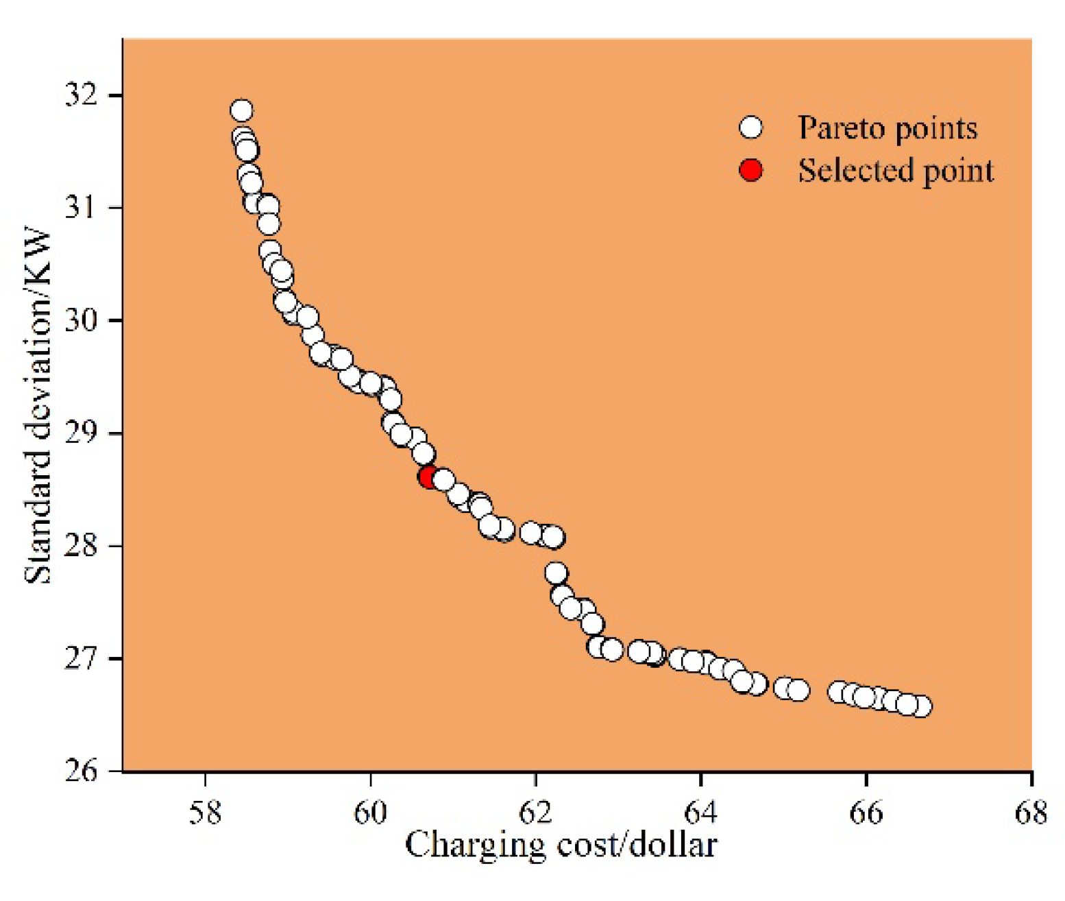
Dual objective	60.7204	28.6401 kW

shows the optimization results obtained by considering the cost of charging for EV users as the single objective function. As a result, the EV user’s charging cost was reduced by 47.42%, and the variance of the load curve decreased by 8.24%. In the case of considering both the EV user’s charging cost and the variance of the load curve as the objective functions, the EV user’s charging cost was reduced by 41.76%, and the variance of the load curve decreased by 31.07%.

These findings demonstrate the effectiveness of the GA and NSGA-II algorithms in optimizing the charging scheduling process for EVs. The optimization results indicate significant improvements in reducing the charging cost for users and minimizing the fluctuations in the load curve.

The results highlight the effectiveness of optimizing EV charging scheduling by considering EV user behavior. The optimization outcomes clearly indicate significant improvements in reducing both EV charging costs and load curve fluctuations.

4. Results and Analysis

The charging behavior portrait categories of EV users were obtained by combining the charging behavior analysis methods for the groups of users and each EV. One or more user charging behavior portrait categories were used to describe the charging behavior of each EV. The accuracy of the charging behavior analysis of EV users was improved.

Based on user priority, one or more user groups can be selected for scheduling. In order to enhance the efficiency of EV dispatch, it is recommended to exclude irregular users; the remaining user groups can be chosen based on the grid’s demand and user satisfaction.

As shown in

Table 10. Charging scheduling sequence based on user charging behavior profile.

	Weekday EVs		Weekend EVs
Vehicle ID	515, 558, 559, 560, 562, 620, 668, 676,832, 1095, 1124, 1137, 1534, 1912, 1083, 567, 714, 69, 2170, 1126, 632, 2461, 850, 569, 1470, 588, 1104, 945, 1001, 1154, 1164, 1524, 431, 818, 712, 1099, 324, 1366, 1154, 777, 609, 1202, 1222, 754, 1135, 1083, 838, 891, 1161, 743, 1746, 1133, 1108		777, 609, 248, 1222, 754, 1135, 1083, 838, 891, 1161, 743, 1746, 1133, 1108, 1202
Valley period (23:00–8:00)	Category 1	1099, 754	754
	Category 2	1133, 1746, 1161, 777, 1164	1133, 1746, 1161, 777
	Category 3	1108, 1202	1108, 1202
	Irregular EVs	1135, 838	1135, 838
Flat period (8:00–12:00) (19:00–23:00)	Category 1	324, 1083, 567, 858, 1126	1083
	Category 2	743, 676, 712, 559, 1164, 620, 69, 891, 558, 818, 714, 945, 1912, 562, 1534, 1104, 1095, 632, 1133, 1124, 560, 1222	743, 891, 1133, 1222
	Category 3	2170, 1366, 1108, 668, 1154, 2461, 569, 850, 431, 832	1108
	Irregular EVs	1524, 1001, 1470, 248	248
Peak period (12:00–19:00)	Category 1	609	609
	Category 2	1746, 1124, 1161, 777, 560, 1222, 562	1161, 777, 1222
	Category 3	1202, 832, 1366, 668, 431, 850	1202
	Irregular EVs	515, 838, 1083, 1137, 1135	838, 1135

, the schedulability of orderly charging for EVs is influenced by the regularity of the EV user’s charging behavior. The table likely presents different levels or categories of user charging behavior regularity and the corresponding strength of schedulability for orderly charging.

(1)

High-quality schedulable EV users (Category 1):

According to Table 10, the most prominent profile categories for these EV users account for more than 70% of the total. The EV users’ behavior indicates a high degree of schedulability in EV charging and discharging scheduling and demand-side response. By dividing the charging periods into peak/flat/valley and weekdays/weekends, it becomes feasible to precisely analyze the scheduling potential of each EV during any specific time segment. This analysis facilitates the creation of optimal scheduling plans for the entire scheduling model.

(2)

Medium-quality schedulable EV users (Category 2):

According to Table 10, these EV users’ two most prominent profile categories account for more than 70% of the total. The EV user’s behavior can be classified into two distinct categories, showing a decrease in regularity and an increase in the randomness of charging behavior. The dispatchability of medium-quality schedulable users is lower compared to that of high-quality schedulable users. If the charging and discharging schedules of high-quality dispatch users fail to meet the power grid’s requirements, further dispatching of medium-quality dispatch users should be considered.

(3)

Low-quality schedulable EV users (Category 3):

According to Table 10, these EV users’ three most prominent profile categories account for more than 70% of the total. The user’s behavior can be categorized into three distinct profiles, with an increase in randomness in charging behavior and a decrease in regularity. The dispatchability of medium-quality dispatch users is higher compared to that of low-quality dispatch users. In the case where the charging and discharging schedules of medium-quality dispatch users are unable to meet the power grid’s requirements, further dispatching of low-quality dispatch users should be considered.

(4)

Irregular users:

Table 10 shows that the sum of the three highest user profile categories in this user category is less than 70%. This user category has a larger number of charging behavior categories, with at least three or more charging behaviors. This indicates a high level of randomness and poor regularity in their charging behavior, further implying that the charging behavior of this user category cannot be analyzed effectively.

According to the analysis in the paper, the regularity of charging habits decreases sequentially from high-quality users to medium-quality users and then to low-quality users. During the scheduling process of EVs with the power grid, it is important to prioritize users with higher priority levels. Such scheduling results are more likely to be accepted by users, thus avoiding any negative impact on user satisfaction and their travel needs. Irregular users, who do not exhibit predictable vehicle usage patterns, are not selected for scheduling due to the inability to learn their behavior.

The impact of user profile classification on the power grid can be manifested in the following aspects:

• Resource allocation: By accurately identifying irregular users as well as high-, medium-, and low-quality schedulable users, resources such as charging stations and grid capacity can be allocated more effectively. High-priority schedulable users could be given priority access to fast charging stations or reserved time slots, while irregular users could be scheduled based on the availability of resources, reducing waiting times, and congestion at charging stations.
• Grid stability: High-priority schedulable users can help grid operators better manage and predict electricity demand. Encouraging these users to charge during periods of low demand or when the generation of renewable energy is high can improve the stability of the grid and maximize the integration of renewable energy sources.
• Demand response programs: Differentiating between user types also enables the implementation of customized demand response programs for each group. Strategies for participating in demand response programs can be formulated based on the priority levels of users, helping to balance grid demand. For irregular users, incentive measures can be introduced to encourage them to adjust their charging patterns, optimizing grid interaction.

Based on the discussion above, this study proposes a method that combines user profiling technology with optimized scheduling for EVs. By utilizing the user profiling model, four different priority levels of user groups are identified, allowing for differentiated settings within the scheduling model. According to the load curve of the scheduling model, it is evident that the user groups meeting the grid demand response play a role in peak shaving and valley filling, validating the feasibility of this strategy. This model significantly enhances the targeted scheduling of EV charging and discharging, improving the interaction efficiency between EVs and the grid.

5. Conclusions

In order to further explore the charging behavior of EVs, this study proposes a method that combines user profiling technology with an EV optimization scheduling model to achieve the precise classification of EV users. The individual feature data, priorities, and group profiles of users are fed into the EV optimization model. The NSGA-II algorithm was employed to solve the scheduling model, and experimental results prove the effectiveness of the proposed optimization strategy. The conclusions are as follows:

(1)

Based on the user profile model, four types of user groups and their priorities were identified, which formed the basis for the differentiated settings of users in the EV scheduling model.

(2)

According to the different priorities of the user groups, the feature values of each EV user were calculated and input into the scheduling model.

(3)

By comparing the EV scheduling model before and after optimization, adjusting the charging times of users effectively reduces charging costs, stabilizes grid load fluctuations, and improves the efficiency of orderly charging, preliminarily verifying the effectiveness of the strategy.

(4)

Based on satisfying user electricity demand and assessing the potential for user response, this study validates the feasibility of certain user group portraits through three charging scheduling scenarios. The experimental results demonstrate that when considering the charging cost of EV users as a single objective function, the charging cost is reduced by 47.42% compared to unstructured charging. When both the charging cost and load fluctuation of EV users are considered as dual objective functions, the charging cost of EV users and the load fluctuation of the charging station are reduced by 41.76% and 31.07%, respectively.

In the future, based on the method of this study, further research will be conducted on integrating renewable energy sources while optimizing EV scheduling to meet the demands of the power grid.

References

- Saleh, M.; Milovanoff, A.; Posen, I.D.; MacLean, H.L.; Hatzopoulou, M. Energy and greenhouse gas implications of shared automated electric vehicles. Transp. Res. Part D Transp. Environ. 2022, 105, 103233. [Google Scholar] [CrossRef]
- Ji, Z.; Huang, X. Plug-in electric vehicle charging infrastructure deployment of China towards 2020: Policies, methodologies, and challenges. Renew. Sustain. Energy Rev. 2018, 90, 710–727. [Google Scholar] [CrossRef]
- IEA. Global EV Outlook 2021; International Energy Agency: Paris, France, 2021. [Google Scholar]
- O’Connell, A.; Flynn, D.; Keane, A. Rolling Multi-Period Optimization to Control Electric Vehicle Charging in Distribution Networks. IEEE PES Gen. Meet. Conf. Expo. 2014, 29, 340–348. [Google Scholar]
- Axsen, J.; Bailey, J.; Castro, M.A. Preference and lifestyle heterogeneity among potential plug-in electric vehicle buyers. Energy Econ. 2015, 50, 190–201. [Google Scholar] [CrossRef]
- Münzel, C.; Plötz, P.; Sprei, F.; Gnann, T. How large is the effect of financial incentives on electric vehicle sales?—A global review and European analysis. Energy Econ. 2019, 84, 104493. [Google Scholar] [CrossRef]
- Yin, W.; Ming, Z.; Wen, T. Scheduling strategy of electric vehicle charging considering different requirements of grid and users. Energy 2021, 232, 121118. [Google Scholar] [CrossRef]
- Muhtadi, A.; Pandit, D.; Nguyen, N.; Mitra, J. Distributed energy resources based microgrid: Review of architecture, control, and reliability. IEEE Trans. Ind. Appl. 2021, 3, 2223–2235. [Google Scholar] [CrossRef]
- Chen, H.; Huang, B. Integrated G2V/V2G switched reluctance motor drive with sensing only switch-bus current. IEEE Trans. Power Electron. 2021, 8, 9372–9381. [Google Scholar] [CrossRef]
- Saber, H.; Ehsan, M.; Moeini-Aghtaie, M.; Fotuhi-Firuzabad, M.; Lehtonen, M. Network-constrained transactive coordination for plug-in electric vehicles participation in real-time retail electricity markets. IEEE Trans. Sustain. Energy 2021, 2, 1439–1448. [Google Scholar] [CrossRef]
- Dong, C.; Chu, R.; Morstyn, T.; McCulloch, M.D.; Jia, H. Online rolling evolutionary decoder-dispatch framework for the secondary frequency regulation of time-varying electrical-grid-electric-vehicle system. IEEE Trans. Smart Grid 2021, 1, 871–884. [Google Scholar] [CrossRef]
- Gan, L.; Topcu, U.; Low, S.H. Optimal decentralized protocol for electric vehicle charging. IEEE Trans. Power Syst. 2013, 2, 940–951. [Google Scholar] [CrossRef]
- Solanke, T.U.; Ramachandaramurthy, V.K.; Yong, J.Y.; Pasupuleti, J.; Kasinathan, K.; Rajagopalan, A. A review of strategic charging–discharging control of grid-connected electric vehicles. J. Energy Storage 2020, 28, 101193. [Google Scholar] [CrossRef]
- Yong, J.Y.; Tan, W.S.; Khorasany, M.; Razzaghi, R. Electric vehicles destination charging: An overview of charging tariffs, business models and coordination strategies. Renew. Sust. Energy. Rev. 2023, 184, 113534. [Google Scholar] [CrossRef]
- Cheng, S.; Wei, Z.; Shang, D.; Zhao, Z.; Chen, H. Charging Load Prediction and Distribution Network Reliability Evaluation Considering Electric Vehicles’ Spatial-Temporal Transfer Randomness. IEEE Access 2020, 8, 124084–124096. [Google Scholar] [CrossRef]
- Huang, A.; Mao, Y.; Chen, X.; Xu, Y.; Wu, S. A multi-timescale energy scheduling model for microgrid embedded with differentiated electric vehicle charging management strategies. Sustain. Cities Soc. 2024, 101, 105123. [Google Scholar] [CrossRef]
- Singh, S.; Vaidya, B.; Mouftah, H.T. Smart EV Charging Strategies Based on Charging Behavior. Front. Energy Res. 2022, 10, 773440. [Google Scholar] [CrossRef]
- Kim, J.D. Insights into residential EV charging behavior using energy meter data. Energy Pol. 2019, 129, 610–618. [Google Scholar] [CrossRef]
- Weldon, P.; Morrissey, P.; Brady, J.; O’Mahony, M. An investigation into usage patterns of electric vehicles in Ireland. Transp. Res Transp. Env. 2016, 43, 207–225. [Google Scholar] [CrossRef]
- Sun, X.-H.; Yamamoto, T.; Morikawa, T. Charge timing choice behavior of battery electric vehicle users. Transp. Res. Transp. Environ. 2015, 37, 97–107. [Google Scholar] [CrossRef]
- Zhou, Y.; Wen, R.; Wang, H.; Cai, H. Optimal battery electric vehicles range: A study considering heterogeneous travel patterns, charging behaviors, and access to charging infrastructure. Energy 2020, 197, 116945. [Google Scholar] [CrossRef]
- Gschwendtner, C.; Knoeri, C.; Stephan, A. The impacts of plug-in behavior on the spatial–temporal flexibility of electric vehicle charging load. Sustain. Cities Soc. 2023, 88, 104263. [Google Scholar] [CrossRef]
- Tian, J.; Lv, Y.; Zhao, Q.; Gong, Y.; Li, C.; Ding, H.; Yu, Y. Electric vehicle charging load prediction considering the orderly charging. Energy Rep. 2022, 8, 124–134. [Google Scholar] [CrossRef]
- Williams, B.; Bishop, D.; Hooper, G.; Chase, J. Driving change: Electric vehicle charging behavior and peak loading. Renew. Sustain. Energy Rev. 2024, 189, 113953. [Google Scholar] [CrossRef]
- Chen, J.; Ai, Q.; Xiao, F. Electric vehicle charging station planning based on user travel demand. Electr. Power Autom. Equip. 2016, 36, 34–39. [Google Scholar]
- Philipsen, R.; Brell, T.; Brost, W.; Eickels, T.; Ziefle, M. Running on empty—Users’ charging behavior of electric vehicles versus traditional refueling. Transp. Res. Part F Traffic Psychol. Behav. 2018, 59, 475–492. [Google Scholar] [CrossRef]
- Wei, W.; Wu, D.; Wu, Q.; Shafie-Khah, M.; Catalão, J.P.S. Interdependence between transportation system and power distribution system: A comprehensive review on models and applications. J. Mod. Power Syst. Clean Energy 2019, 7, 433–448. [Google Scholar] [CrossRef]
- Wei, W.; Mei, S.; Wu, L.; Shahidehpour, M.; Fang, Y. Optimal traffic-power flow in urban electrified transportation networks. IEEE Trans. Smart Grid 2017, 8, 84–95. [Google Scholar] [CrossRef]
- Yao, W.; Zhao, J.; Wen, F.; Dong, Z.; Xue, Y.; Xu, Y.; Meng, K. A multi-objective collaborative planning strategy for integrated power distribution and electric vehicle charging systems. IEEE Trans. Power Syst. 2014, 9, 1811–1821. [Google Scholar] [CrossRef]
- Wang, X.; Shahidehpour, M.; Jiang, C.; Li, Z. Coordinated planning strategy for electric vehicle charging stations and coupled traffic-electric networks. IEEE Trans. Power Syst. 2019, 34, 268–279. [Google Scholar] [CrossRef]
- Hou, K.; Xu, X.; Jia, H.; Yu, X.; Jiang, T.; Zhang, K.; Shu, B. A reliability assessment approach for integrated transportation and electrical power systems incorporating electric vehicles. IEEE Trans. Smart Grid 2018, 9, 88–100. [Google Scholar] [CrossRef]
- Meng, J.; Mu, Y.; Jia, H.; Wu, J.; Yu, X.; Qu, B. Dynamic frequency response from electric vehicles considering travelling behavior in the Great Britain power system. Appl. Energy 2016, 162, 966–979. [Google Scholar] [CrossRef]
- How, D.N.T.; Hannan, M.A.; Hossain Lipu, M.S.; Ker, P.J. State of charge estimation for lithium-ion batteries using model-based and data-driven methods: A review. IEEE Access 2019, 7, 136116–136136. [Google Scholar] [CrossRef]
- Xydas, E.; Marmaras, C.; Cipcigan, L.M.; Jenkins, N.; Carroll, S.; Barker, M. A A data driven approach for characterizing the charging demand of electric vehicles: A UK case study. Appl. Energy 2016, 162, 763–771. [Google Scholar] [CrossRef]
- Liu, Y.; Wang, J. Multi-source Data Driven Electric Vehicle User Identification Method. Electr. Power Syst. Autom. 2023, 35, 141–147. [Google Scholar]
- Bui, V.-H.; Hussain, A.; Zarrabian, S.; Kump, P.M.; Su, W. Clustering-based optimal operation of charging stations under high penetration of electric vehicles. Sustain. Energy Grids Netw. 2023, 36, 101178. [Google Scholar] [CrossRef]
- Xu, J.; Feng, G.; Zhao, T.; Sun, X.; Zhu, M. Remote sensing image classification based on semi-supervised adaptive interval Type-2 fuzzy C-Means algorithm. Comput. Geosci. 2019, 131, 132–143. [Google Scholar] [CrossRef]
- Li, S.; Cheng, Y.; Lin, S. A FCM-based deterministic forecasting model for fuzzy time series. Comput. Math. Appl. 2008, 12, 3052–3063. [Google Scholar] [CrossRef]
- Xiong, Y.; Wang, B.; Chu, C.-C.; Gadh, R. Vehicle grid integration for demand response with mixture user model and decentralized optimization. Appl. Energy 2018, 231, 481–493. [Google Scholar] [CrossRef]
- Chung, Y.-W.; Khaki, B.; Li, T.; Chu, C.; Gadh, R. Ensemble machine learning-based algorithm for electric vehicle user behavior prediction. Appl. Energy 2019, 254, 113732. [Google Scholar] [CrossRef]
- Chen, Y.; Li, Y.; Shen, Y. Industrial customer group portrait method based on potential quantization model of load control. Electr. Power Autom. Equip. 2021, 41, 208–216. [Google Scholar]
- Vagropoulos, S.I.; Keranidis, S.D.; Afentoulis, K.D.; Bampos, Z.N.; Laitsos, V.M. Electric vehicle smart charging business case-outcomes and prospects for electric vehicle aggregators. In Proceedings of the 2023 19th International Conference on the European Energy Market (EEM), Lappeenranta, Finland, 6–8 June 2023; pp. 1–7. [Google Scholar]
- Wang, R.; Mu, J.; Sun, Z.; Wang, J.; Hu, A. NSGA-II multi-objective optimization regional electricity price model for electric vehicle charging based on travel law. Energy Rep. 2021, 7, 1495–1503. [Google Scholar] [CrossRef]
- Yi, Z.; Liu, X.C.; Wei, R.; Chen, X.; Dai, J. Electric vehicle charging demand forecasting using deep learning model. J. Intell. Transp. Syst. 2022, 26, 690–703. [Google Scholar] [CrossRef]
- Lee, Z.J.; Pang, J.Z.; Low, S.H. Pricing EV charging service with demand charge. Electr. Power Syst. Res. 2020, 189, 106694. [Google Scholar] [CrossRef]
- He, Y.; Liu, Z.; Song, Z. Joint optimization of electric bus charging infrastructure, vehicle scheduling, and charging management. Transp. Res. D Transp. Environ. 2023, 117, 103653. [Google Scholar] [CrossRef]