
The Electrochemical Commercial Vehicle (ECCV) Platform
 , , and
Abstract
:1. Introduction
2. Challenges, Aim and Method
3. Overview of the Platform and Its Components
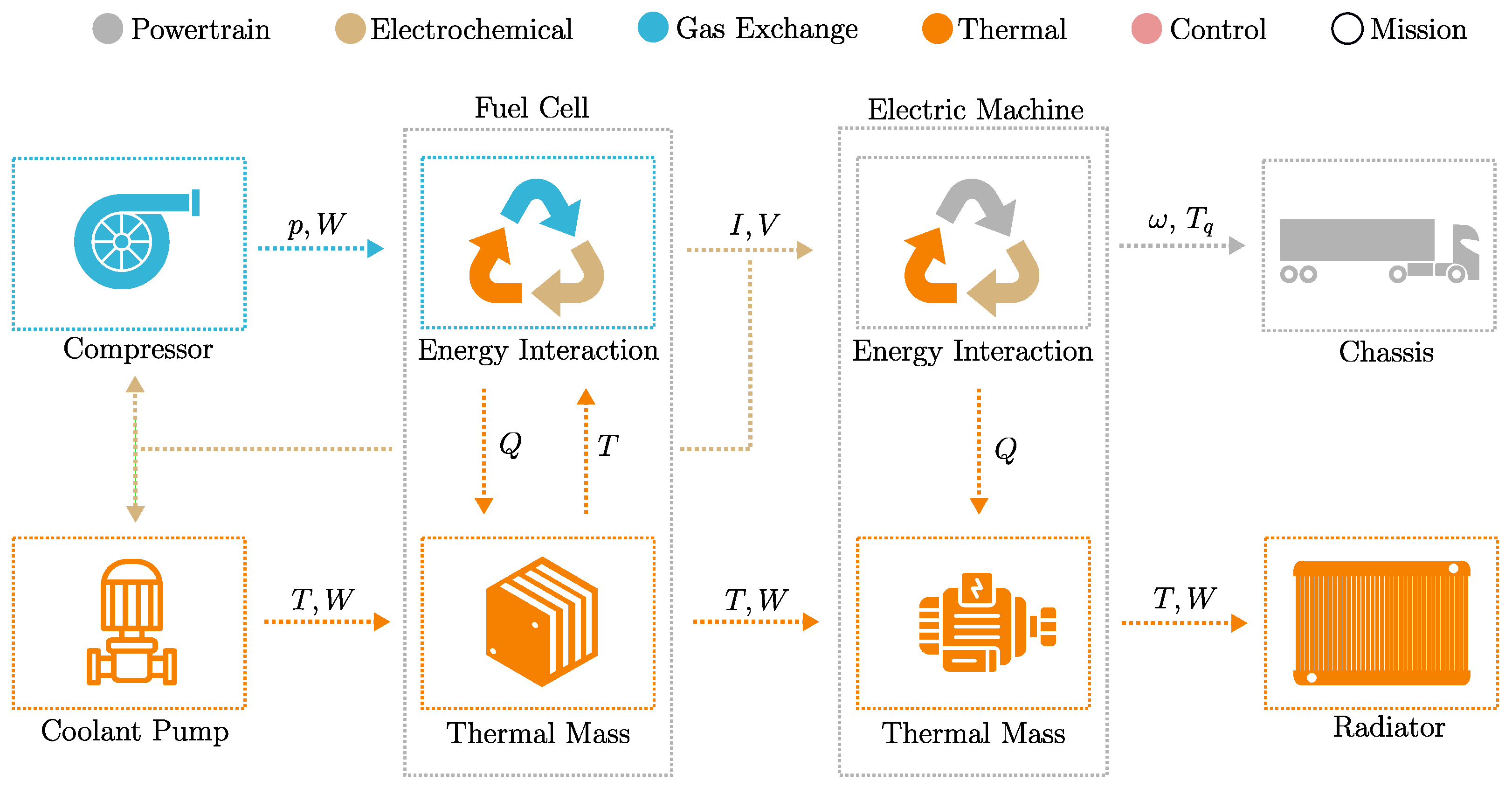
3.1. Library Structure and Model Interfaces
3.1.1. Driving Missions
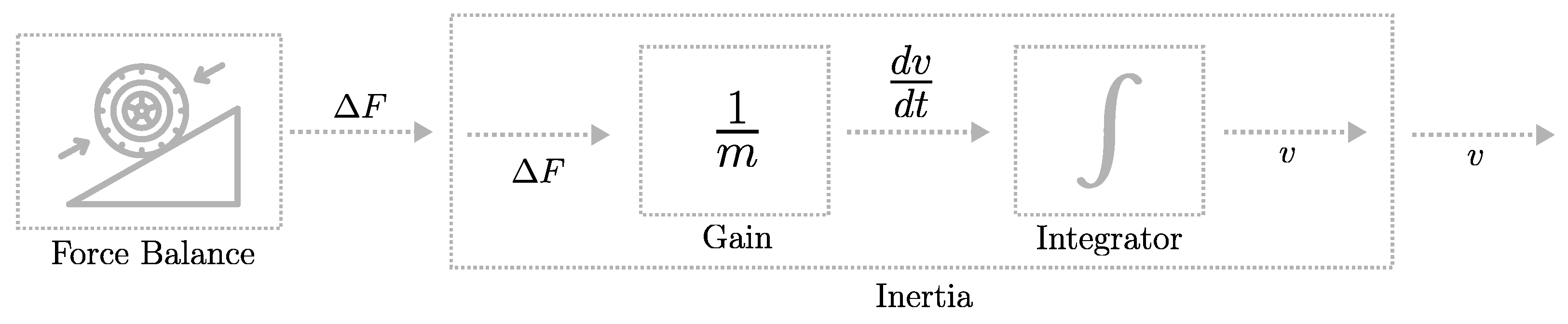
3.1.2. Powertrain
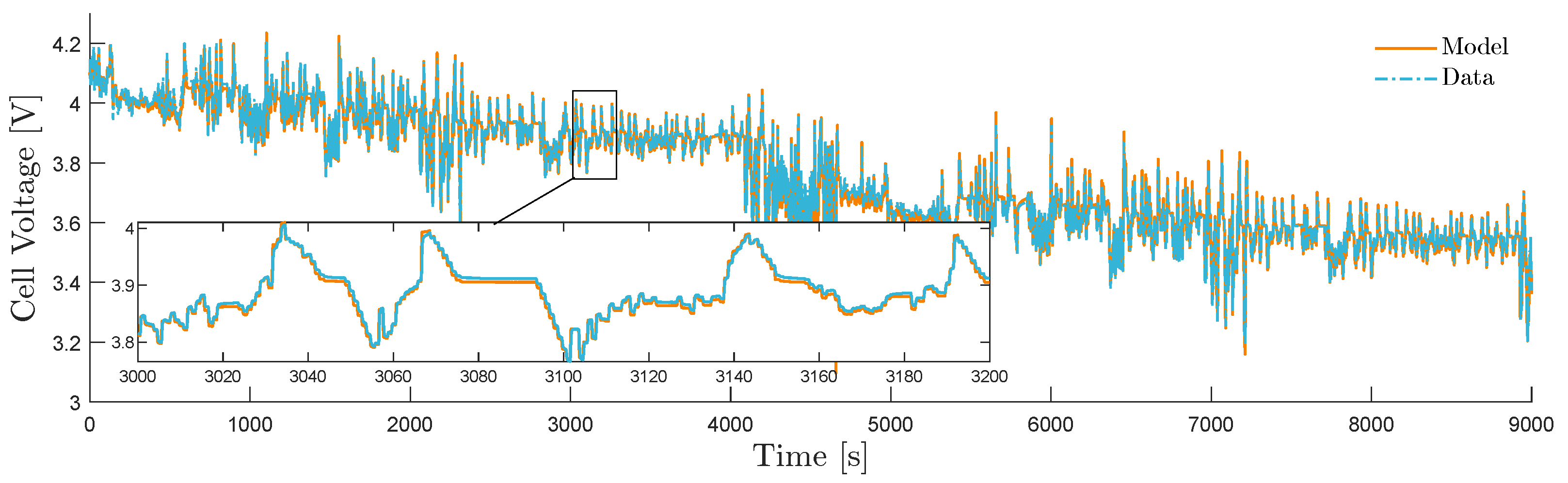
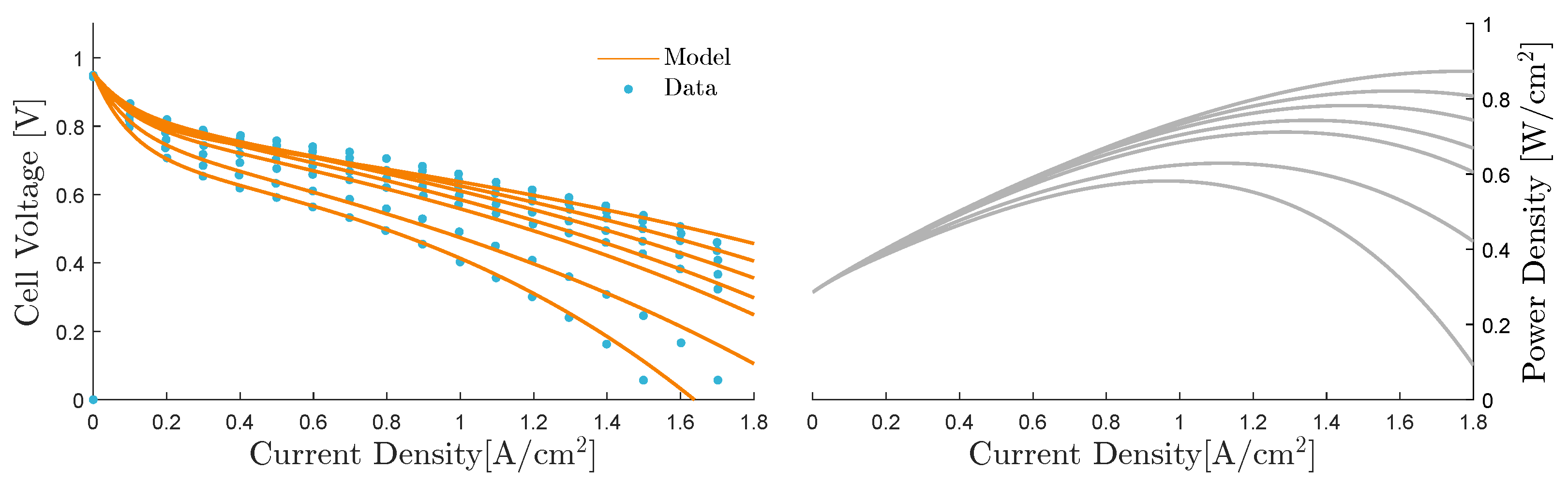
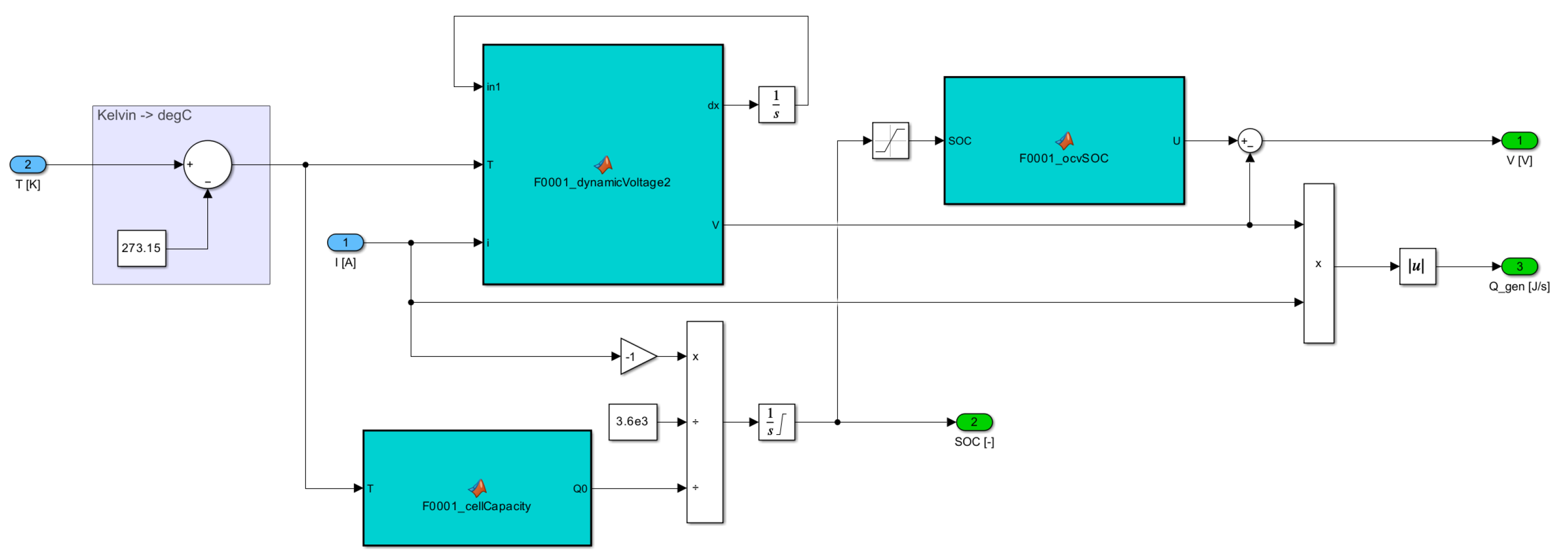
3.1.3. Electrochemical
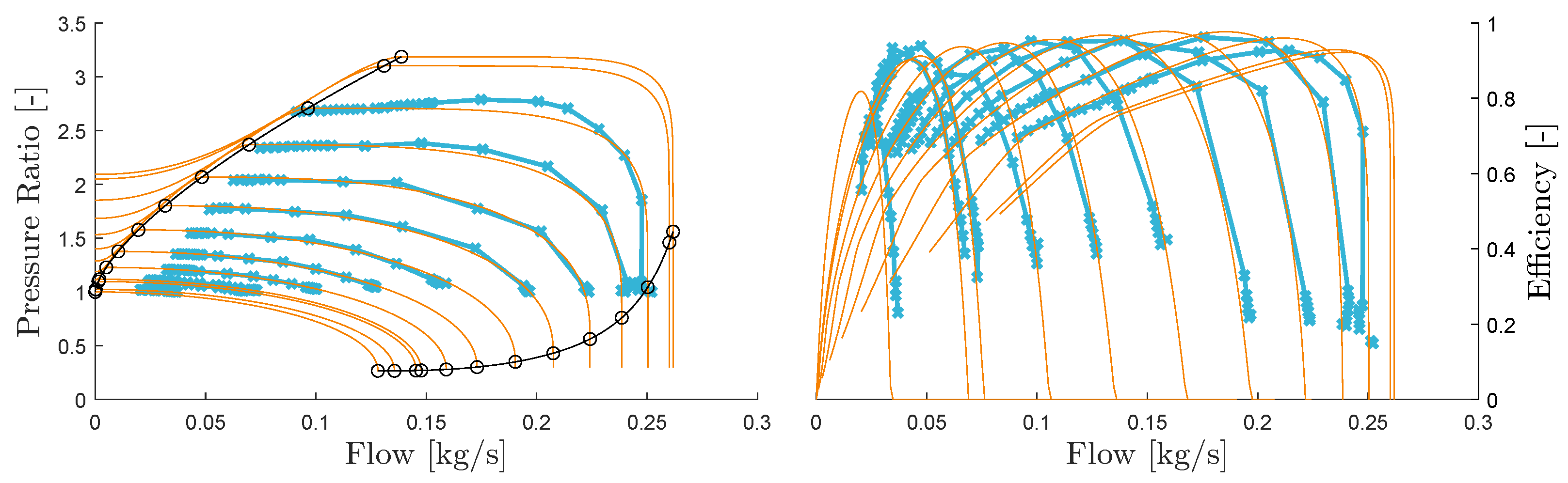
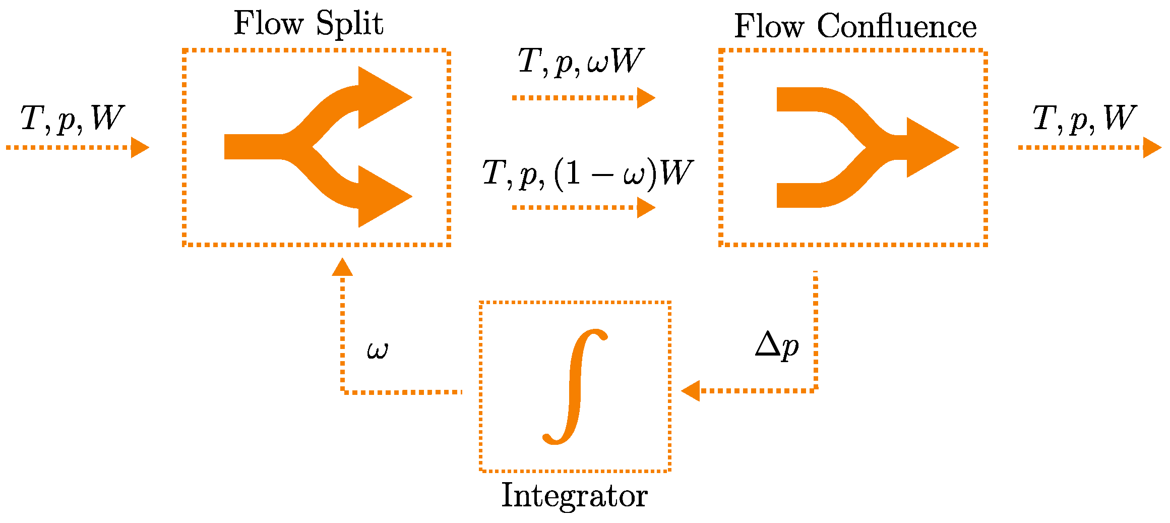
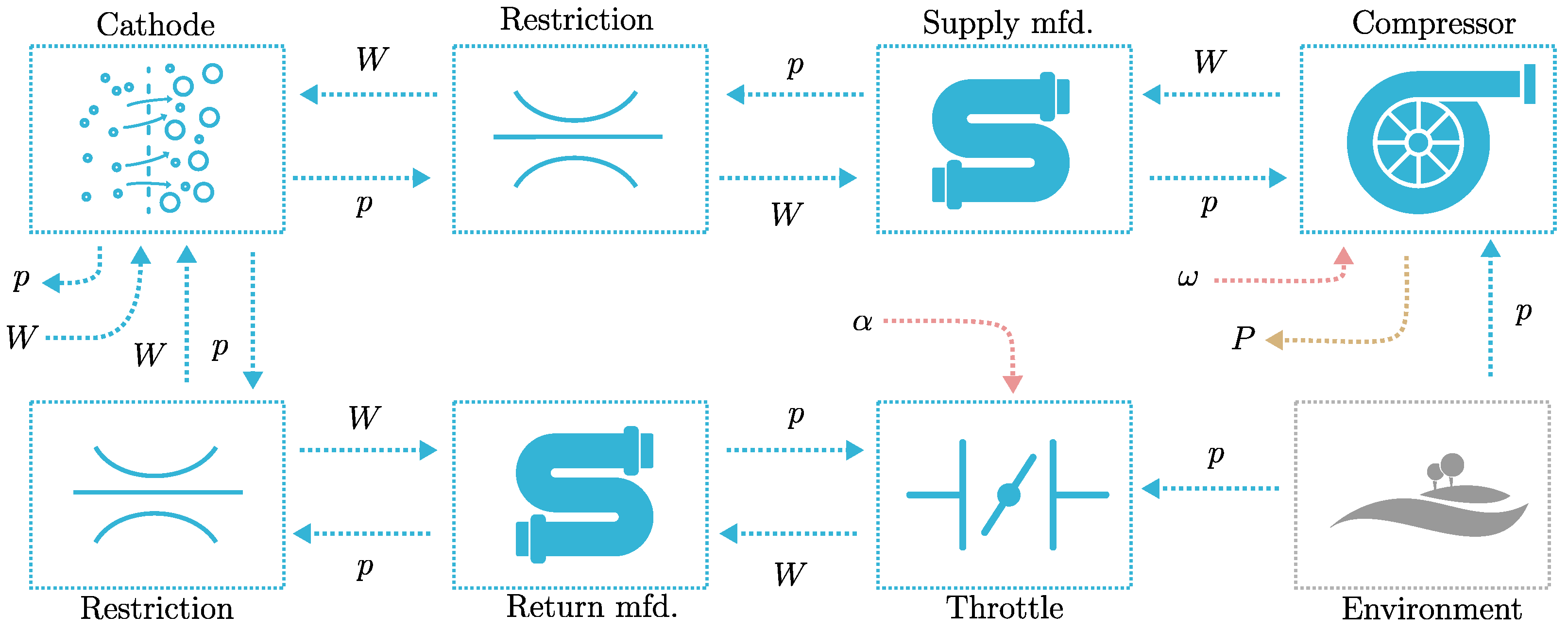
3.1.4. Gas Exchange
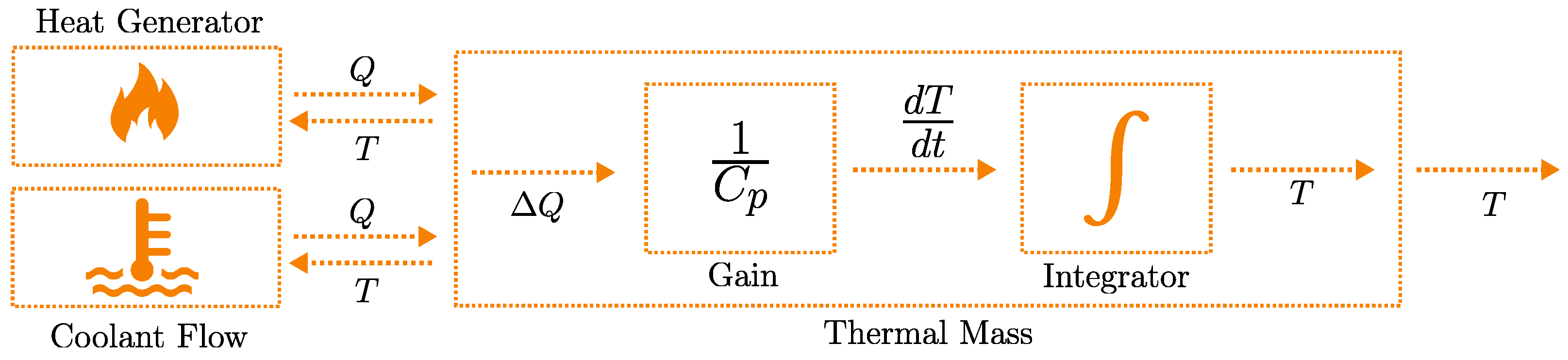
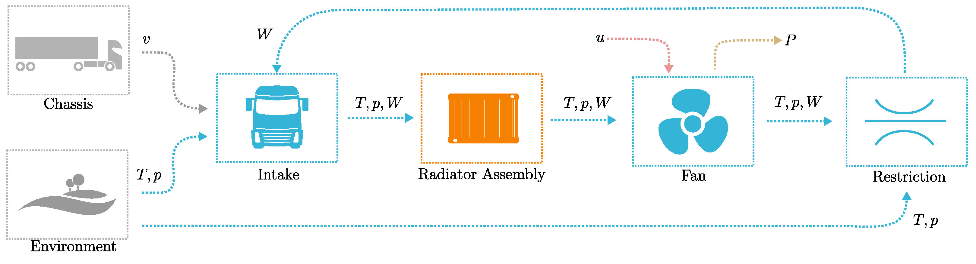
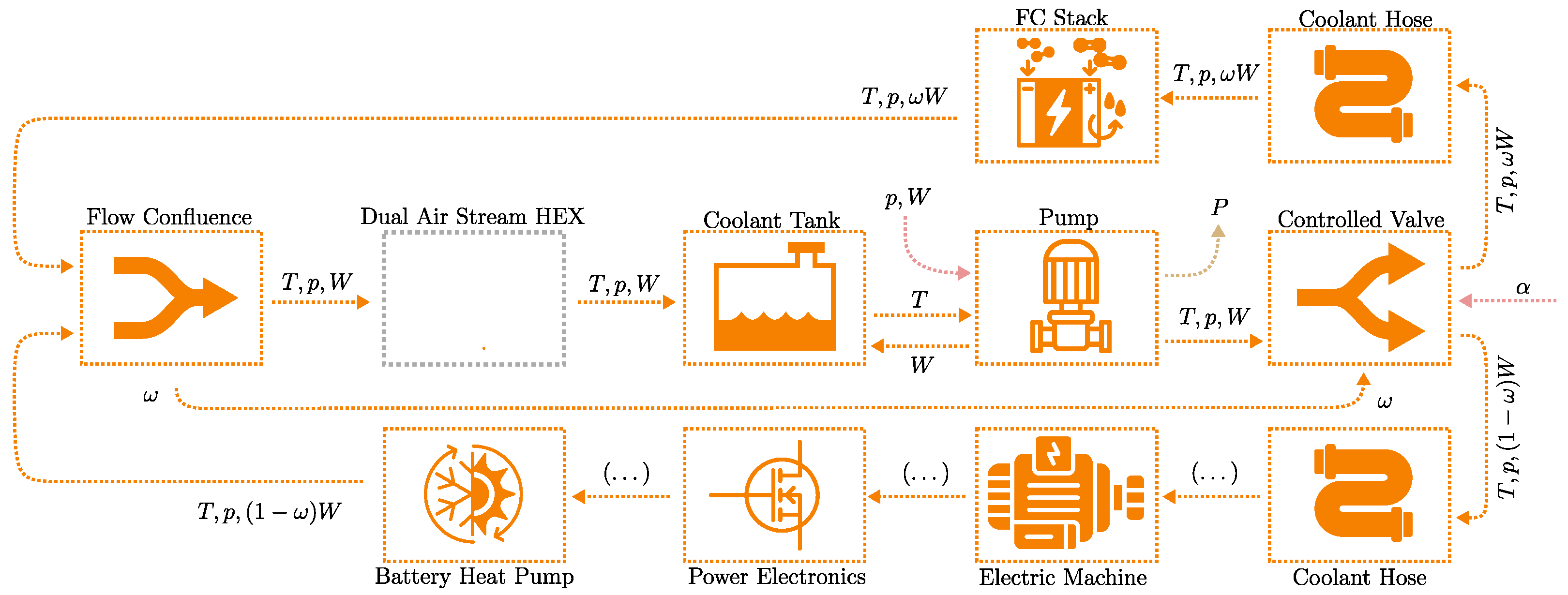
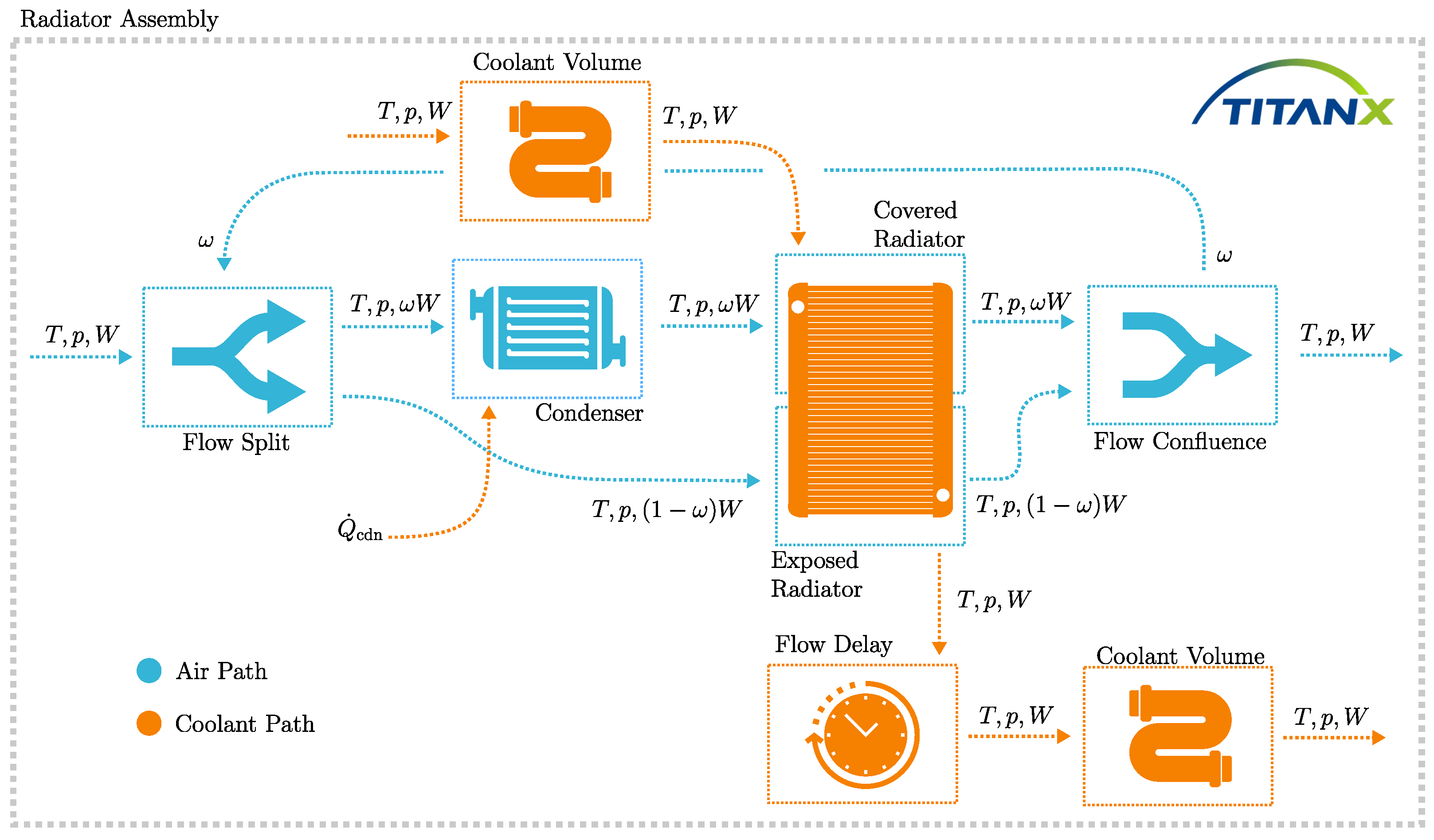
3.1.5. Thermal
3.1.6. Control
4. Vehicle System Example Models
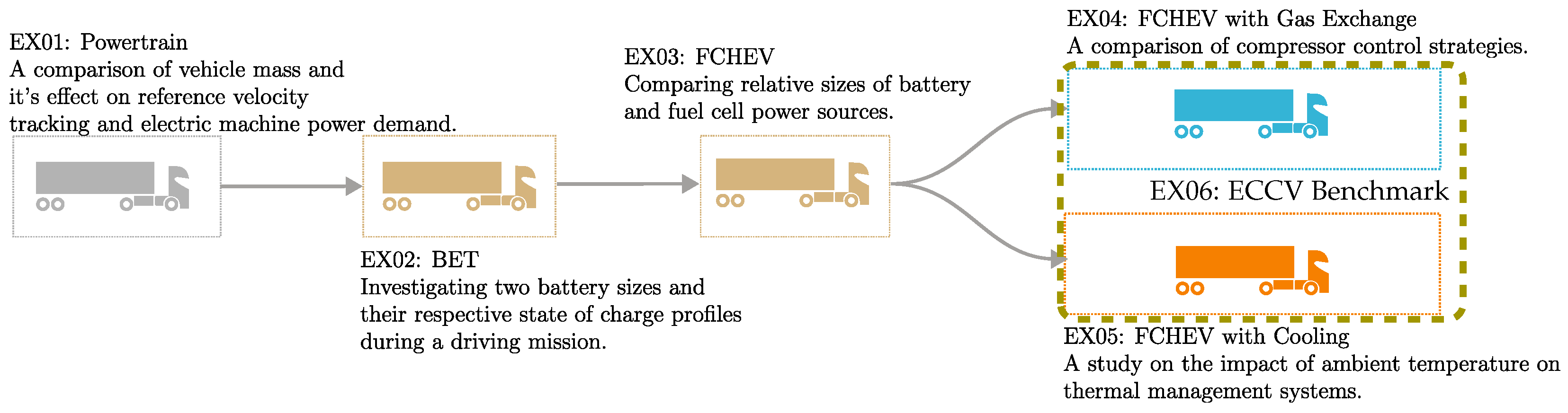
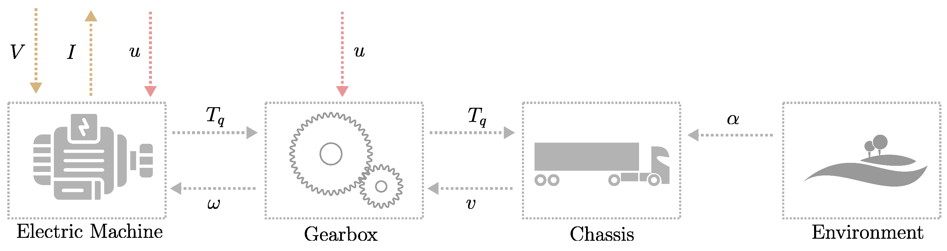
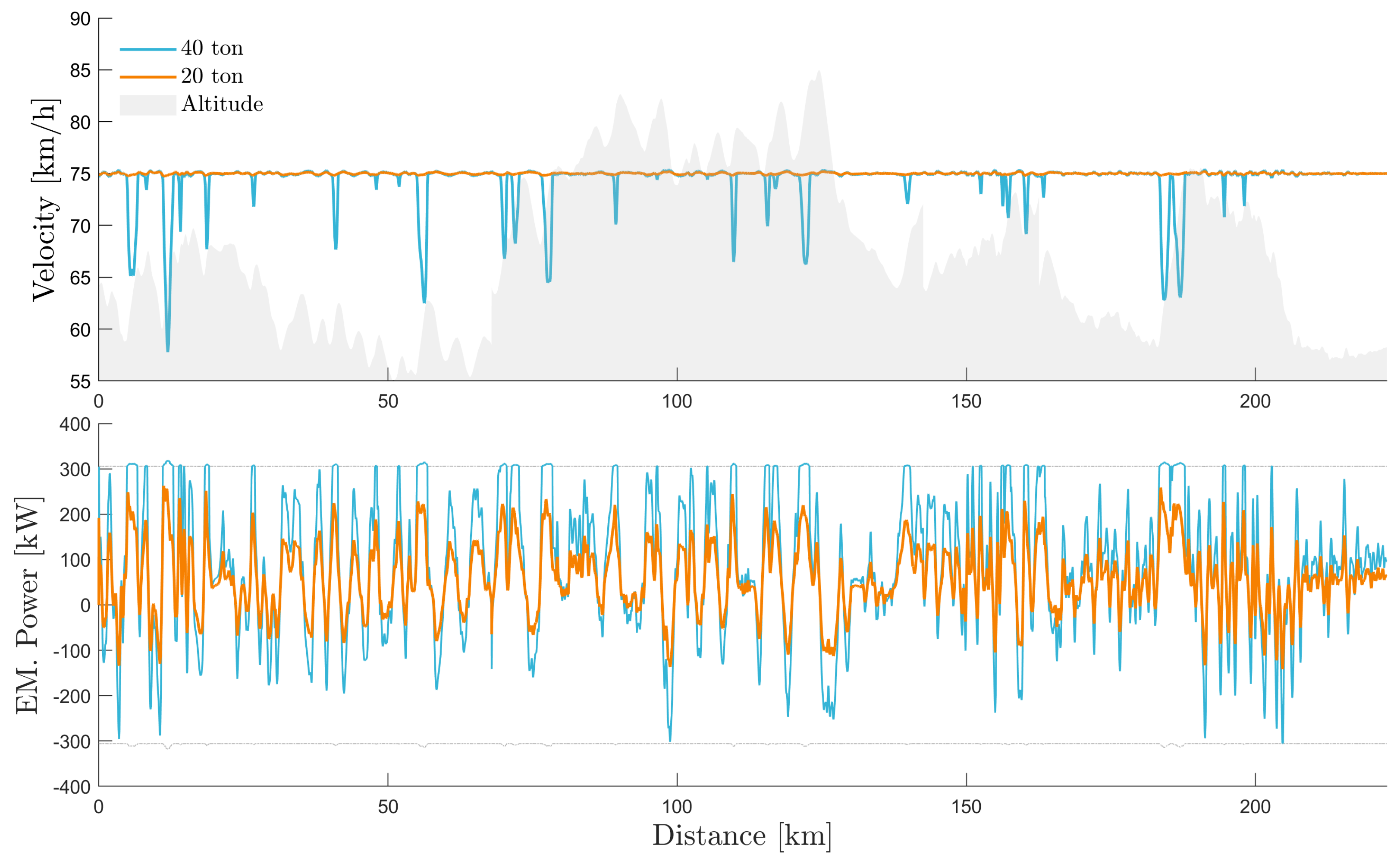
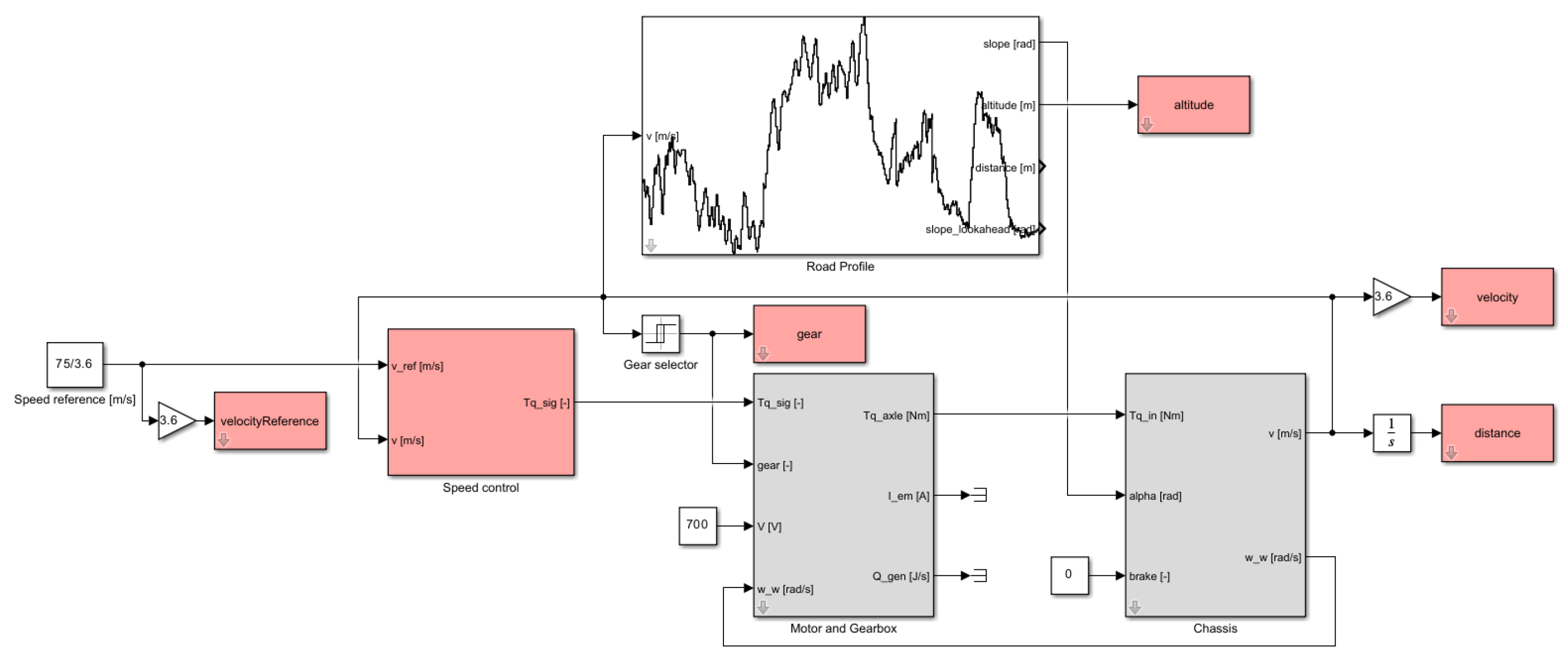
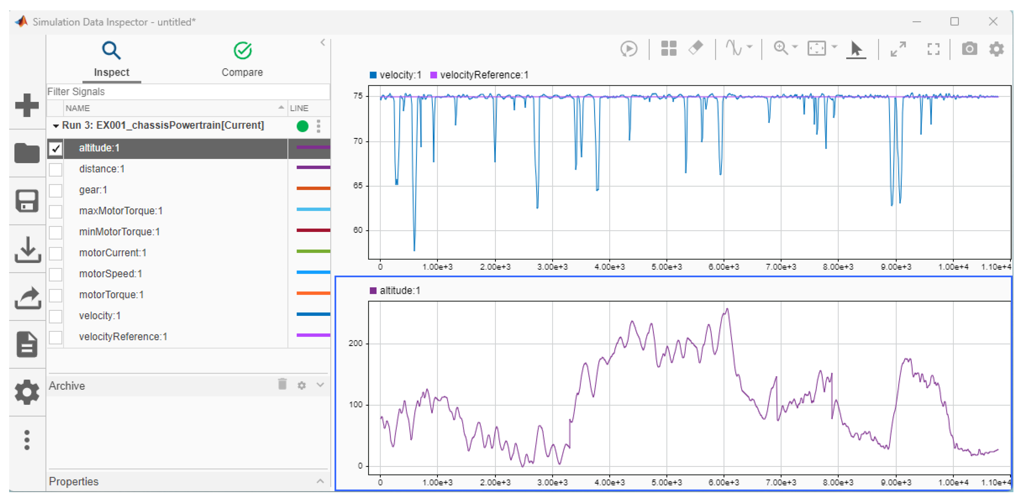
4.1. Example 1: Chassis and Powertrain
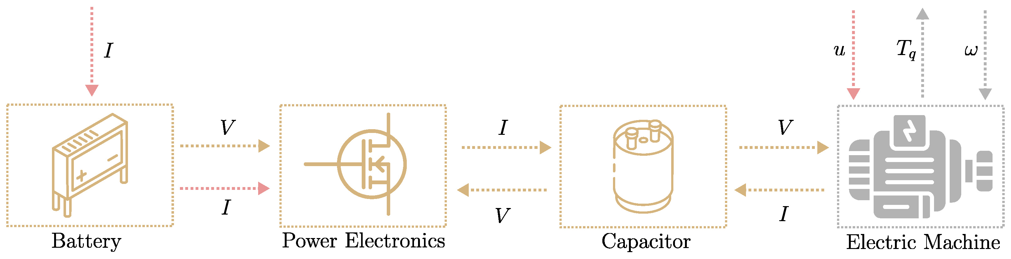
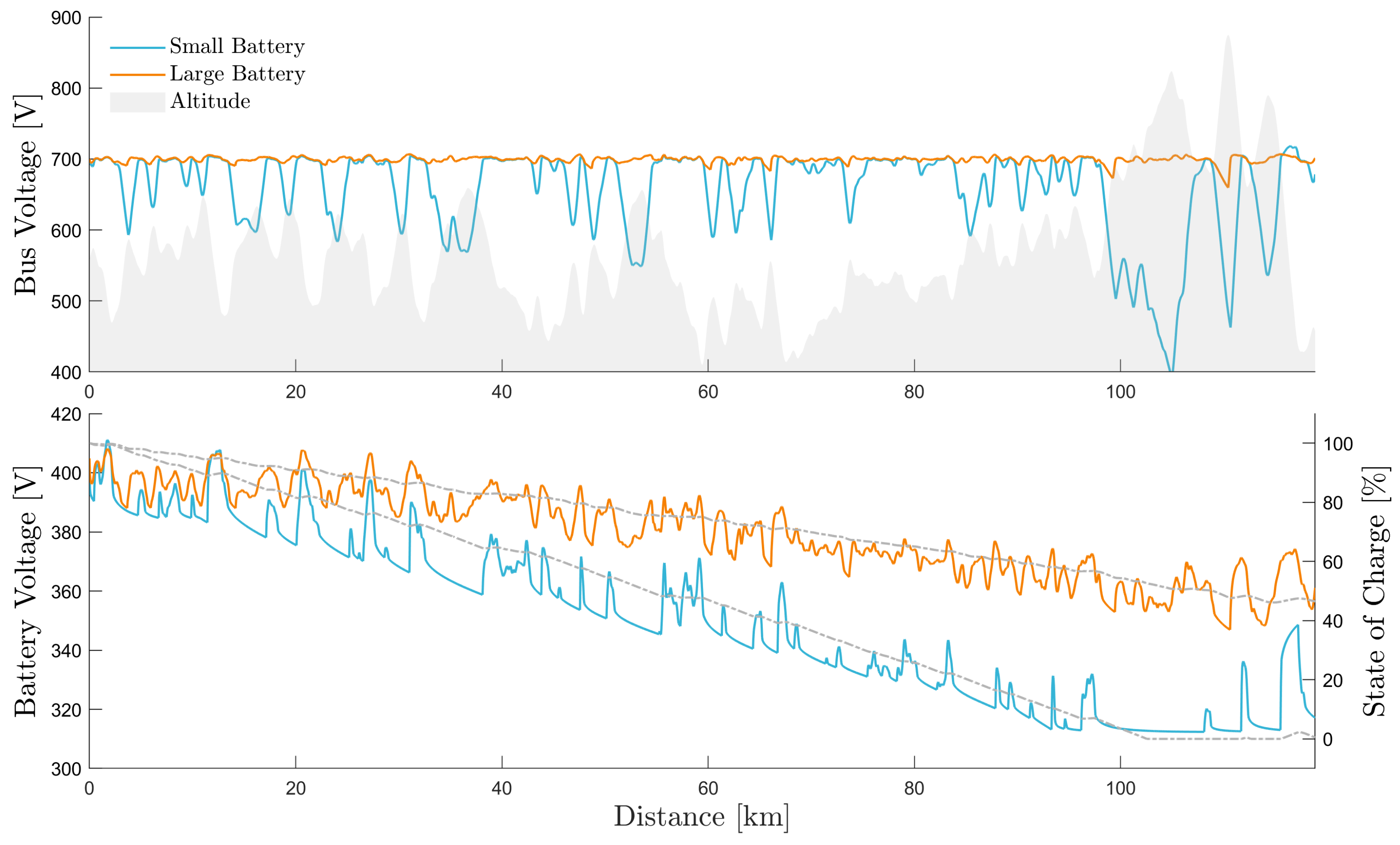
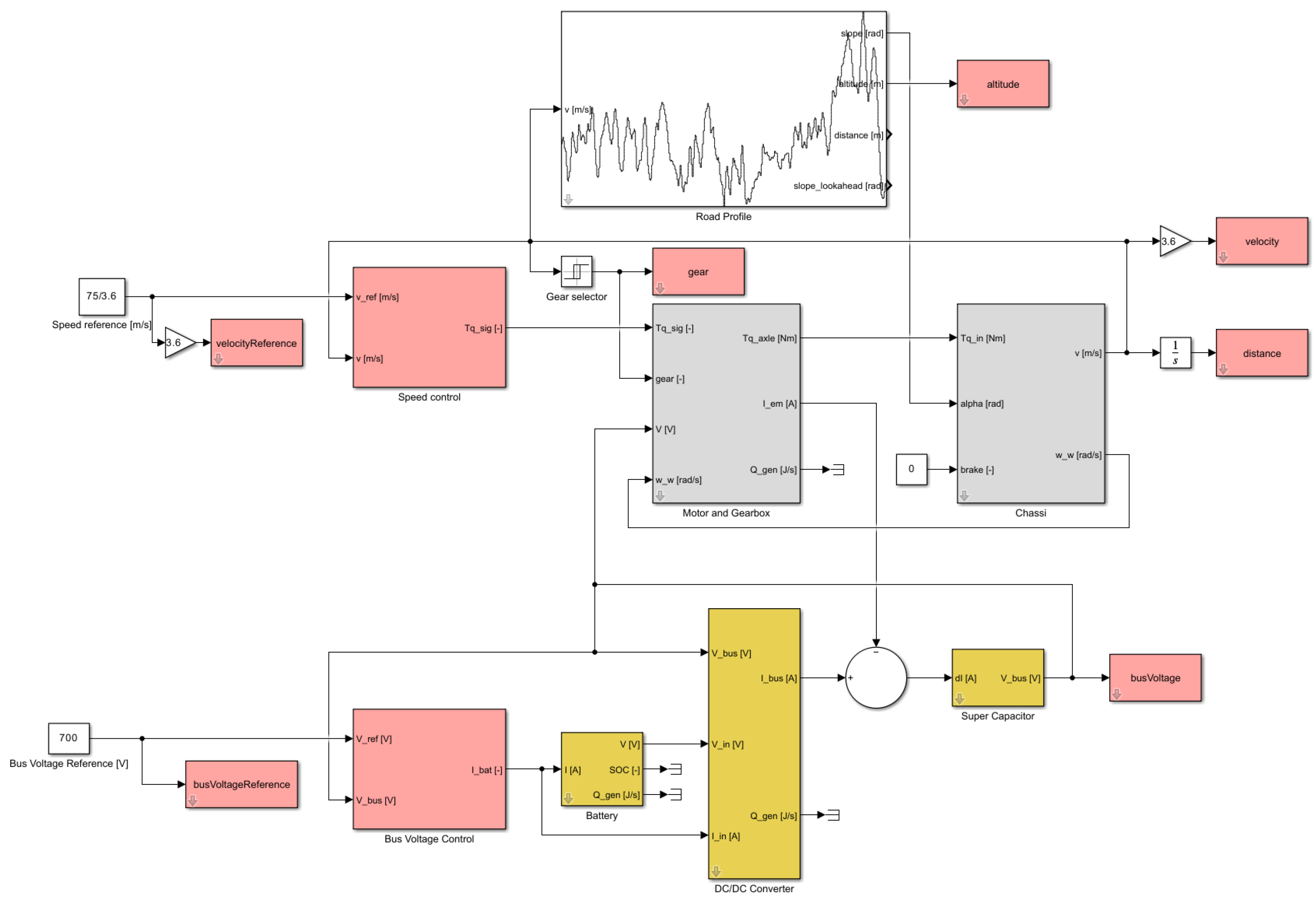
4.2. Example 2: Battery Electric Truck
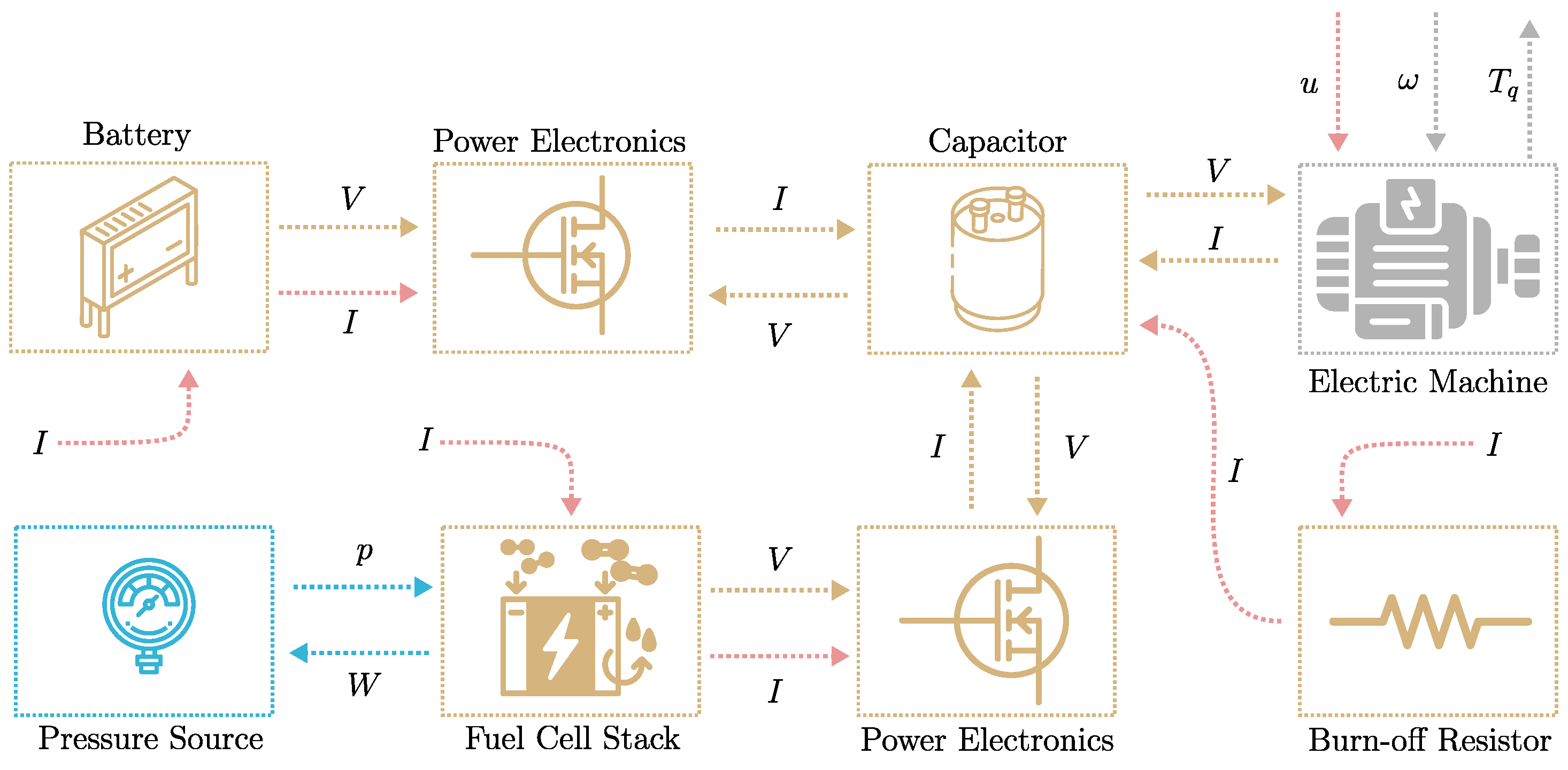
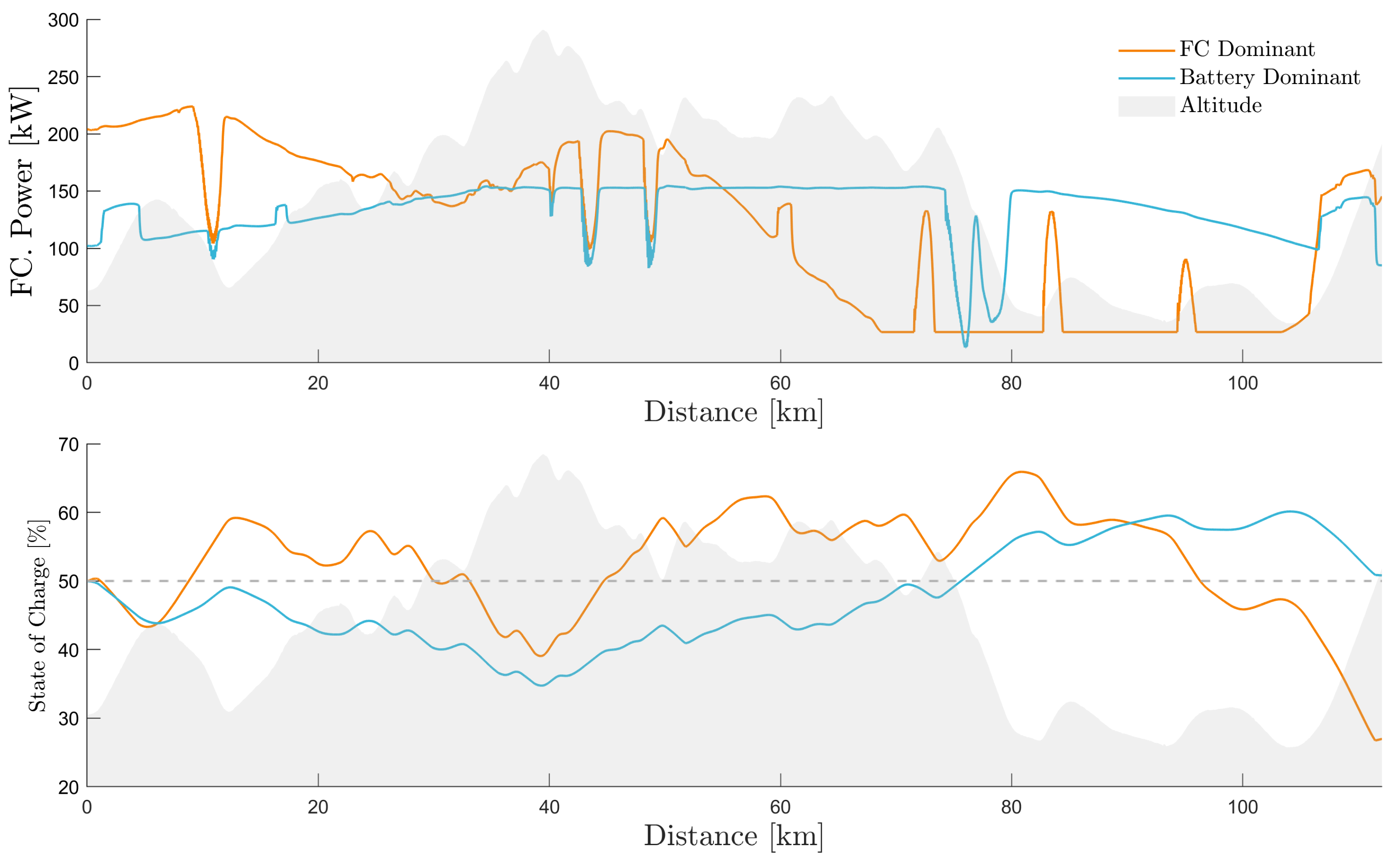
4.3. Example 3: FCHEV
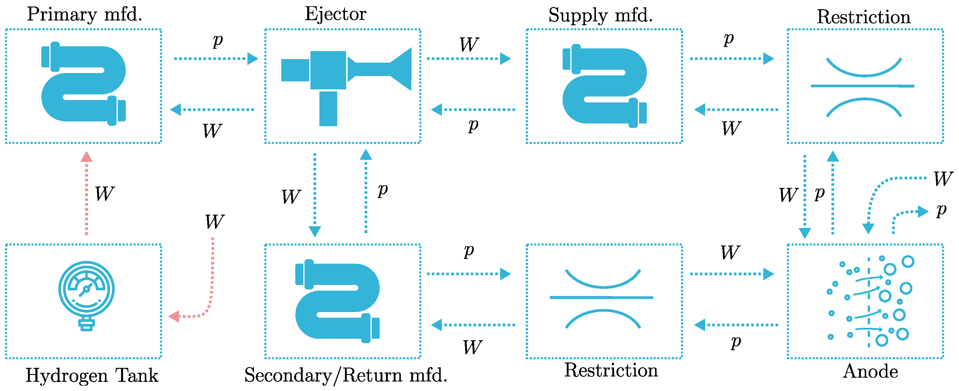
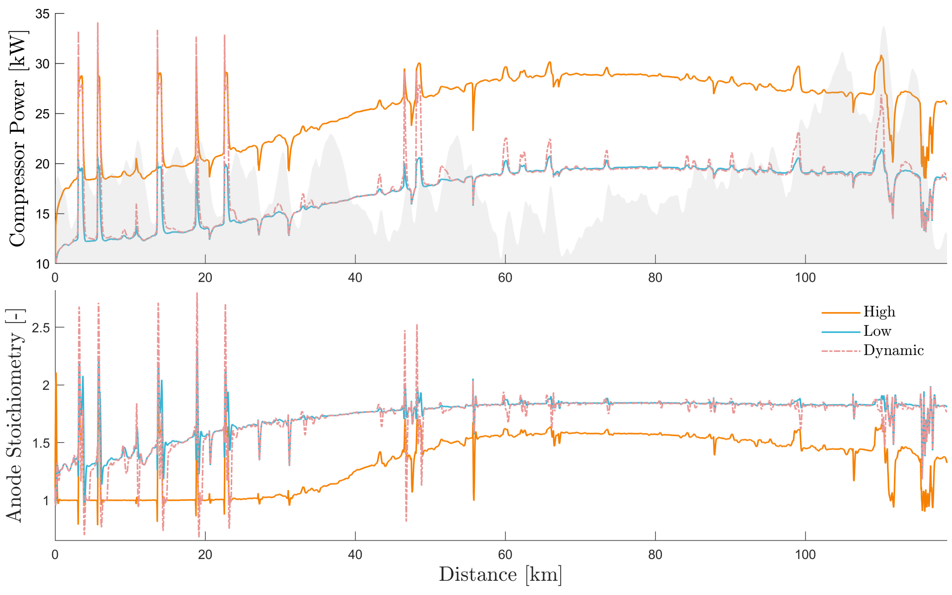
4.4. Example 4: FCHEV with Gas Exchange
4.5. Example 5: FCHEV with Cooling
4.6. Example 6: ECCV Control Benchmark
5. Results and Discussion
6. Conclusions
Author Contributions
Funding
Data Availability Statement
Acknowledgments
Conflicts of Interest
Appendix A. Simulink Implementation


References
- Luo, Y.; Wu, Y.; Li, B.; Mo, T.; Li, Y.; Feng, S.P.; Qu, J.; Chu, P.K. Development and application of fuel cells in the automobile industry. J. Energy Storage 2021, 42, 103124. [Google Scholar] [CrossRef]
- Peters, R.; Breuer, J.L.; Decker, M.; Grube, T.; Robinius, M.; Samsun, R.C.; Stolten, D. Future Power Train Solutions for Long-Haul Trucks. Sustainability 2021, 13, 2225. [Google Scholar] [CrossRef]
- Cullen, D.A.; Neyerlin, K.C.; Ahluwalia, R.K.; Mukundan, R.; More, K.L.; Borup, R.L.; Weber, A.Z.; Myers, D.J.; Kusoglu, A. New roads and challenges for fuel cells in heavy-duty transportation. Nat. Energy 2021, 6, 462–474. [Google Scholar] [CrossRef]
- Kast, J.; Vijayagopal, R.; Gangloff, J.J.; Marcinkoski, J. Clean commercial transportation: Medium and heavy duty fuel cell electric trucks. Int. J. Hydrogen Energy 2017, 42, 4508–4517. [Google Scholar] [CrossRef]
- Luo, Y.; Wu, Y.; Li, B.; Qu, J.; Feng, S.P.; Chu, P.K. Optimization and cutting-edge design of fuel-cell hybrid electric vehicles. Int. J. Energy Res. 2021, 45, 18392–18423. Available online: https://onlinelibrary.wiley.com/doi/pdf/10.1002/er.7094 (accessed on 4 February 2024). [CrossRef]
- Pardhi, S.; Chakraborty, S.; Tran, D.D.; El Baghdadi, M.; Wilkins, S.; Hegazy, O. A Review of Fuel Cell Powertrains for Long-Haul Heavy-Duty Vehicles: Technology, Hydrogen, Energy and Thermal Management Solutions. Energies 2022, 15, 9557. [Google Scholar] [CrossRef]
- Chen, Q.; Zhang, G.; Zhang, X.; Sun, C.; Jiao, K.; Wang, Y. Thermal management of polymer electrolyte membrane fuel cells: A review of cooling methods, material properties, and durability. Appl. Energy 2021, 286, 116496. [Google Scholar] [CrossRef]
- Wu, J.; Yuan, X.Z.; Martin, J.J.; Wang, H.; Zhang, J.; Shen, J.; Wu, S.; Merida, W. A review of PEM fuel cell durability: Degradation mechanisms and mitigation strategies. J. Power Sources 2008, 184, 104–119. [Google Scholar] [CrossRef]
- Yue, M.; Jemei, S.; Gouriveau, R.; Zerhouni, N. Review on health-conscious energy management strategies for fuel cell hybrid electric vehicles: Degradation models and strategies. Int. J. Hydrogen Energy 2019, 44, 6844–6861. [Google Scholar] [CrossRef]
- Alpaslan, E.; Çetinkaya, S.A.; Alpaydın, C.Y.; Korkmaz, S.A.; Karaoğlan, M.U.; Colpan, C.O.; Erginer, K.E.; Gören, A. A review on fuel cell electric vehicle powertrain modeling and simulation. Energy Sources Part A Recover. Util. Environ. Eff. 2021, 1–37. [Google Scholar] [CrossRef]
- Lohse-Busch, H.; Stutenberg, K.; Duoba, M.; Liu, X.; Elgowainy, A.; Wang, M.; Wallner, T.; Richard, B.; Christenson, M. Automotive fuel cell stack and system efficiency and fuel consumption based on vehicle testing on a chassis dynamometer at minus 18 degC to positive 35 degC temperatures. Int. J. Hydrogen Energy 2020, 45, 861–872. [Google Scholar] [CrossRef]
- Fischer, T.; Götz, F.; Berg, L.F.; Kollmeier, H.P.; Gauterin, F. Model based Development of a Holistic Thermal Management System for an Electric Car with a High Temperature Fuel Cell Range Extender. In Proceedings of the 11th International Modelica Conference, Versailles, France, 21–23 September 2015; pp. 127–133. [Google Scholar]
- Previati, G.; Mastinu, G.; Gobbi, M. Thermal Management of Electrified Vehicles, A Review. Energies 2022, 15, 1326. [Google Scholar] [CrossRef]
- Brooker, A.; Gonder, J.; Wang, L.; Wood, E.; Lopp, S.; Ramroth, L. FASTSim: A Model to Estimate Vehicle Efficiency, Cost and Performance. In Proceedings of the SAE 2015 World Congress & Exhibition, Detroit, MI, USA, 21–23 April 2015. [Google Scholar] [CrossRef]
- Gamma Technologies, LLC. GT-SUITE. 2024. Available online: https://www.gtisoft.com/ (accessed on 4 February 2024).
- Wang, Y.; Li, J.; Tao, Q.; Bargal, M.H.S.; Yu, M.; Yuan, X.; Su, C. Thermal Management System Modeling and Simulation of a Full-Powered Fuel Cell Vehicle. J. Energy Resour. Technol. 2019, 142, 061304. [Google Scholar] [CrossRef]
- Sandrini, G.; Gadola, M.; Chindamo, D. Longitudinal Dynamics Simulation Tool for Hybrid APU and Full Electric Vehicle. Energies 2021, 14, 1207. [Google Scholar] [CrossRef]
- Meyer, J.; Kiss, T.; Chaney, L. A New Automotive Air Conditioning System Simulation Tool Developed in MATLAB/Simulink. SAE Int. J. Passeng. Cars-Mech. Syst. 2013, 6, 826–840. [Google Scholar] [CrossRef]
- Kiss, T.; Lustbader, J. Comparison of the Accuracy and Speed of Transient Mobile A/C System Simulation Models. SAE Int. J. Passeng. Cars Mech. Syst. 2014, 7, 739–754. [Google Scholar] [CrossRef]
- Kiss, T.; Lustbader, J.; Leighton, D. Modeling of an Electric Vehicle Thermal Management System in MATLAB/Simulink; SAE Technical Paper 2015-01-1708; SAE International: Warrendale, PA, USA, 2015. [Google Scholar] [CrossRef]
- Titov, G.; Lustbader, J.; Leighton, D.; Kiss, T. MATLAB/Simulink Framework for Modeling Complex Coolant Flow Configurations of Advanced Automotive Thermal Management Systems; SAE Technical Paper 2016-01-0230; SAE International: Warrendale, PA, USA, 2016. [Google Scholar] [CrossRef]
- Titov, G.; Lustbader, J.A. Modeling Control Strategies and Range Impacts for Electric Vehicle Integrated Thermal Management Systems with MATLAB/Simulink. In Proceedings of the WCX™ 17: SAE World Congress Experience, Detroit, MI, USA, 4–6 March 2017. [Google Scholar] [CrossRef]
- Kirpes, B.; Danner, P.; Basmadjian, R.; Meer, H.d.; Becker, C. E-mobility systems architecture: A model-based framework for managing complexity and interoperability. Energy Inform. 2019, 2, 1–31. [Google Scholar] [CrossRef]
- Eriksson, L.; Thomasson, A.; Ekberg, K.; Reig, A.; Eifert, M.; Donatantonio, F.; D’Amato, A.; Arsie, I.; Pianese, C.; Otta, P.; et al. Look-ahead controls of heavy duty trucks on open roads—Six benchmark solutions. Control Eng. Pract. 2019, 83, 45–66. [Google Scholar] [CrossRef]
- Kollmeyer, P.; Hackl, A.; Emadi, A. Li-ion battery model performance for automotive drive cycles with current pulse and EIS parameterization. In Proceedings of the 2017 IEEE Transportation Electrification Conference and Expo (ITEC), Chicago, IL, USA, 22–24 June 2017; pp. 486–492. [Google Scholar] [CrossRef]
- Zhang, C.; Jiang, J.; Zhang, L.; Liu, S.; Wang, L.; Loh, P.C. A Generalized SOC-OCV Model for Lithium-Ion Batteries and the SOC Estimation for LNMCO Battery. Energies 2016, 9, 900. [Google Scholar] [CrossRef]
- Kollmeyer, P. Panasonic 18650PF Li-ion Battery Data. Mendeley Data 2018, V1. [Google Scholar] [CrossRef]
- MathWorks. MATLAB System Identification Toolbox. 2024. Available online: https://www.mathworks.com/ (accessed on 4 February 2024).
- Pukrushpan, J.T.; Peng, H.; Stefanopoulou, A.G. Control-Oriented Modeling and Analysis for Automotive Fuel Cell Systems. J. Dyn. Syst. Meas. Control 2004, 126, 14–25. [Google Scholar] [CrossRef]
- Leufvén, O.; Eriksson, L. A Surge and Choke Capable Compressor Flow Model—Validation and Extrapolation Capability. Control Eng. Pract. 2013, 21, 1871–1883. [Google Scholar] [CrossRef]
- Llamas, X.; Eriksson, L. LiU CPgui: A Toolbox for Parameterizing Compressor Models; Linköping University Electronic Press: Linköping, Sweden, 2018. [Google Scholar]
- Llamas, X.; Eriksson, L. Parameterizing Compact and Extensible Compressor Models Using Orthogonal Distance Minimization. J. Eng. Gas Turbines Power 2016, 139, 012601. [Google Scholar] [CrossRef]
- Kuo, J.K.; Hsieh, C.Y. Numerical investigation into effects of ejector geometry and operating conditions on hydrogen recirculation ratio in 80 kW PEM fuel cell system. Energy 2021, 233, 121100. [Google Scholar] [CrossRef]
- Wang, X.; Xu, S.; Xing, C. Numerical and experimental investigation on an ejector designed for an 80 kW polymer electrolyte membrane fuel cell stack. J. Power Sources 2019, 415, 25–32. [Google Scholar] [CrossRef]
- Holman, J. Heat Transfer, 10th ed.; McGraw-Hill Education: New York, NY, USA, 2010. [Google Scholar]


| Variable | Description | Variable | Description |
|---|---|---|---|
| W | Mass flow | P | Power |
| p | Pressure, partial pressure | I | Electrical current |
| V | Voltage | T | Temperature |
| Torque | Angular velocity, flow split fraction | ||
| F | Force | v | Longitudinal velocity |
| m | Mass | V | Volume |
| Q | Heat flow | Heat capacity | |
| u | System input | Road slope |
| Parameter | Ex. 1 | Ex. 2 | Ex. 3 | Ex. 4 | Ex. 5 | Unit |
|---|---|---|---|---|---|---|
| Mass | 20/40 | 40 | 40 | 40 | 40 | ton |
| EM Rated Power | 360 | 360 | 360 | 360 | 360 | kW |
| Speed Ref. | 75 | 75 | 75 | 75 | 75 | km/h |
| Bus Voltage Ref. | 700 | 700 | 700 | 700 | V | |
| Bat. Capacity | 450/900 | 360/180 | 360 | 360 | Ah | |
| Bat. Max. Current | 1 | 1 | 1 | 1 | C | |
| Conv. Efficiency | 0.99 | 0.99 | 0.99 | 0.99 | ||
| FC. Stack Power | 240/480 | 240 | 240 | kW | ||
| FC. Max. Current | 600 | 600 | 600 | A | ||
| FC. Pressure Ref. | 2.5 | 2.5/3.5 | 2.5 | bar | ||
| SOC. Ref. | 50 | 50 | 50 | % | ||
| Cath. Stoich. Ref. | 2 | |||||
| Amb. Temp. | 20 | 20/40 | °C | |||
| FC. Mass | 72 | kg | ||||
| FC. Heat Capacity | 420 | J/K | ||||
| Coolant Flow | 4 | kg/s | ||||
| Radiator Area | 1 | m2 | ||||
| Radiator Depth | 52 | mm |
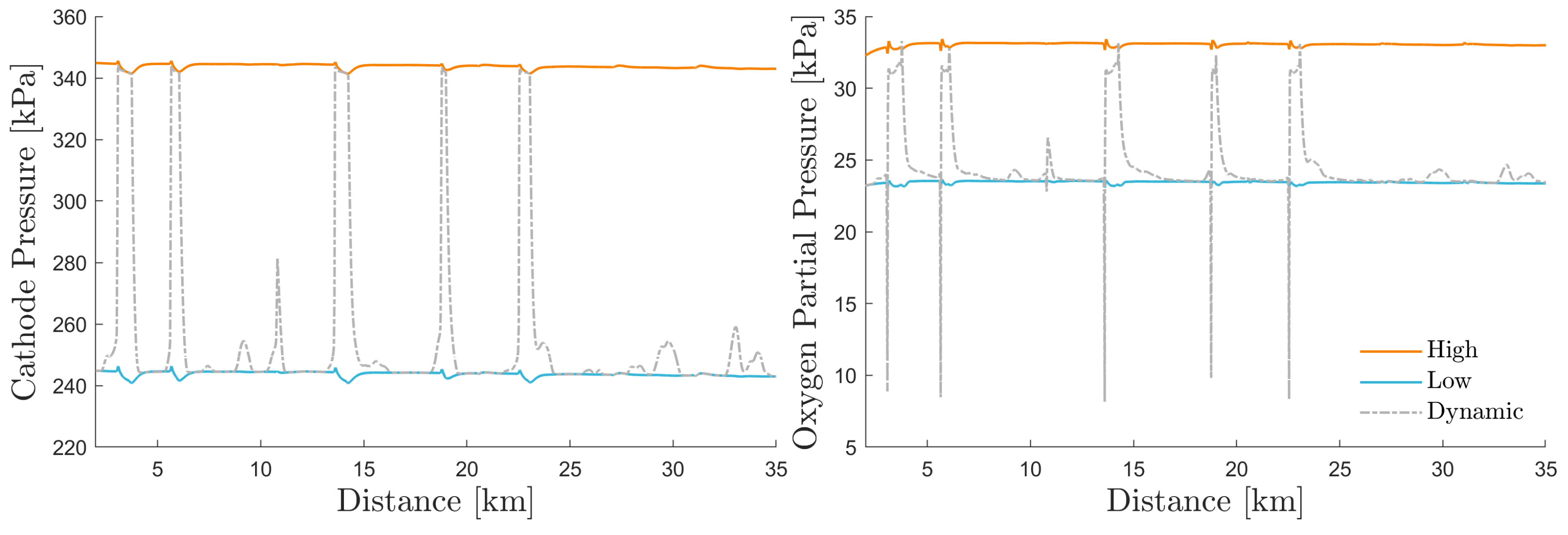
| Pressure | Low | Dynamic | High | |
|---|---|---|---|---|
| Pressure reference | 2.5 | 3.5 | bar | |
| Fuel Consumption | 13.00 | 12.89 | 12.57 | kg |
Disclaimer/Publisher’s Note: The statements, opinions and data contained in all publications are solely those of the individual author(s) and contributor(s) and not of MDPI and/or the editor(s). MDPI and/or the editor(s) disclaim responsibility for any injury to people or property resulting from any ideas, methods, instructions or products referred to in the content. |
© 2024 by the authors. Licensee MDPI, Basel, Switzerland. This article is an open access article distributed under the terms and conditions of the Creative Commons Attribution (CC BY) license (https://creativecommons.org/licenses/by/4.0/).
Share and Cite
Johansson, M.; Contet, A.; Erlandsson, O.; Holmbom, R.; Höckerdal, E.; Jonsson, O.L.; Jung, D.; Eriksson, L. The Electrochemical Commercial Vehicle (ECCV) Platform. Energies 2024, 17, 1742. https://doi.org/10.3390/en17071742
Johansson M, Contet A, Erlandsson O, Holmbom R, Höckerdal E, Jonsson OL, Jung D, Eriksson L. The Electrochemical Commercial Vehicle (ECCV) Platform. Energies. 2024; 17(7):1742. https://doi.org/10.3390/en17071742
Chicago/Turabian StyleJohansson, Max, Arnaud Contet, Olof Erlandsson, Robin Holmbom, Erik Höckerdal, Oskar Lind Jonsson, Daniel Jung, and Lars Eriksson. 2024. "The Electrochemical Commercial Vehicle (ECCV) Platform" Energies 17, no. 7: 1742. https://doi.org/10.3390/en17071742