
A Stochastic Methodology for EV Fast-Charging Load Curve Estimation Considering the Highway Traffic and User Behavior

 , ,
, ,
Abstract
:1. Introduction
2. Literature Review
Paper Contributions
- An adaptative MCS model to estimate user behavior variables of FCS entry probability and charging duration times, considering regional OD patterns, regional influence zones, EV market, user anxiety range, and initial SoC condition.
- Improvements on the traffic flow methodology, considering [17], estimating EVs traveling on the road or highway on a time domain. Since the inputs patterns are stochastic, a discrete matrix model is proposed, with adaptative sizes according to distances and average velocities.
- An FCS operation model, based on charger unit operation matrices, where it considers the charging duration frequency distribution. Like the queue theory model, but increases this approach with recognition of hourly seasonalities, using the traffic results lastly obtained and the relation between EV user and charger technologies.
- To discuss variables affecting FCS load curves on highways, uncertainty points, and analysis about how to apply this load information in planning studies. Also, sensibilities on empirical parameter incentive discussions about secondary influences on FCS operation efficiency.
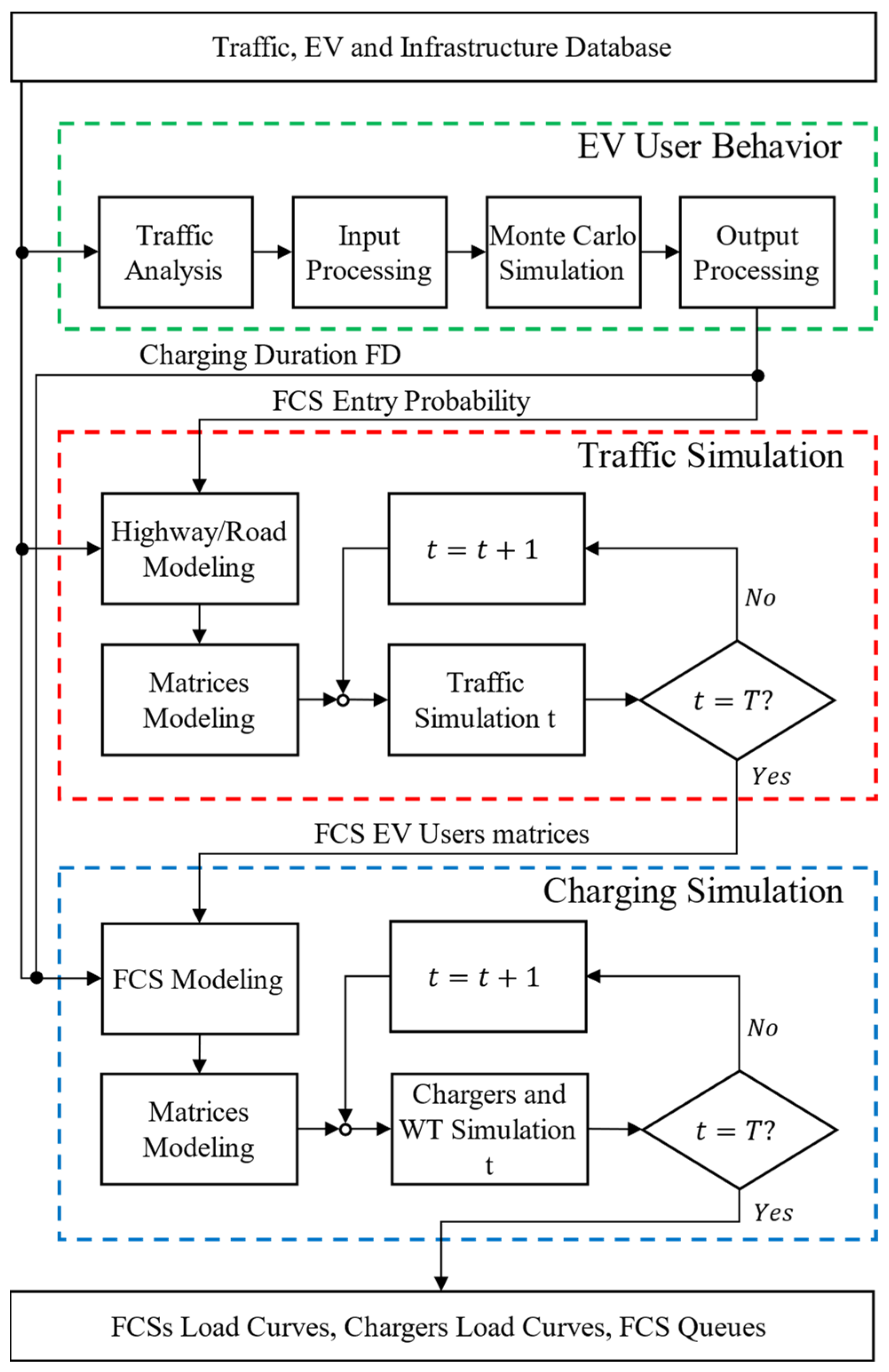
3. Methodology
3.1. EV User Behavior
| Algorithm 1: Pseudocode representation for the user behavior model, returning charging duration frequency distribution and entrance probability |
| Input Input While all FCS are not processed do While stopping criteria not satisfied do 1 to 100 do using (8,9,10,11,12) end and new scenarios using (13) , And , And then else end then Break end end Next FCS end to each FCS |
3.2. Traffic Simulation Model
| Algorithm 2: Pseudocode of the traffic simulation model, composed by the traffic flow and the EV entrance matrix calculation. |
according to (19) according to (15) according to (20) considering results from (22) do do then then else according to (20): do end end end end according to (23): do do then do = True then end end else end end end |
3.3. Fast-Charging Station Model
| Algorithm 3: Pseudocode of the fast-charging station model for the load curve and queue length estimation. |
| While all points are not processed do then according to (25) using (24) do c = 1 > 0 do using (28) = 1 do then Break end end then do end else end end end Calculate the FCS Load Curve using (29) Save the FCS Queue Length like (30) else Next end end |
4. Results and Discussion
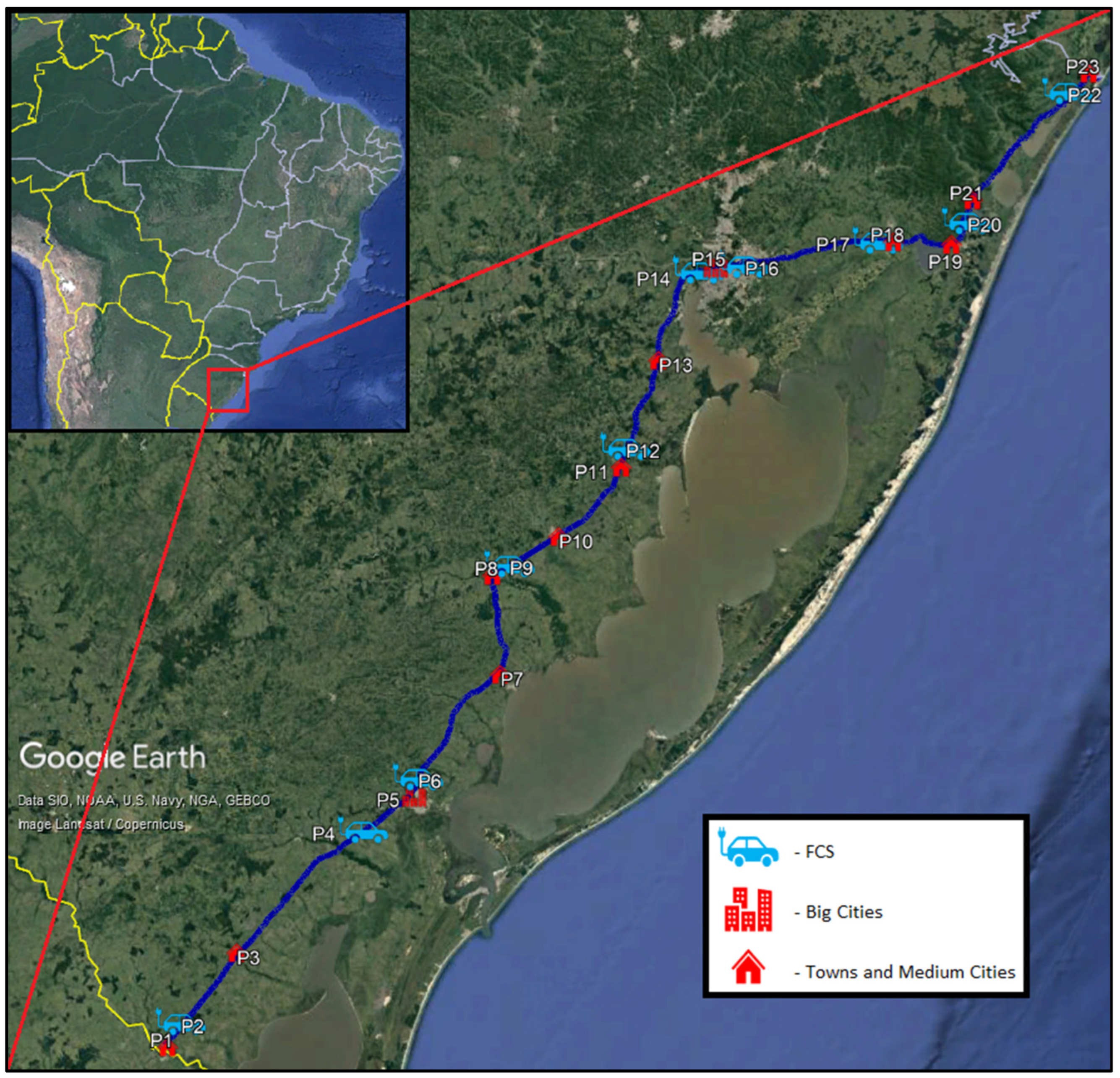
4.1. Case Study
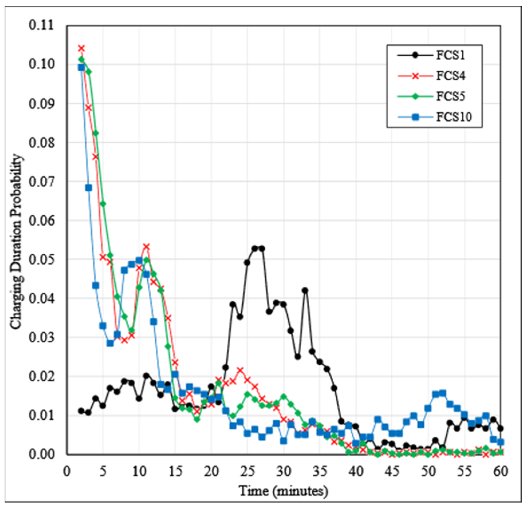
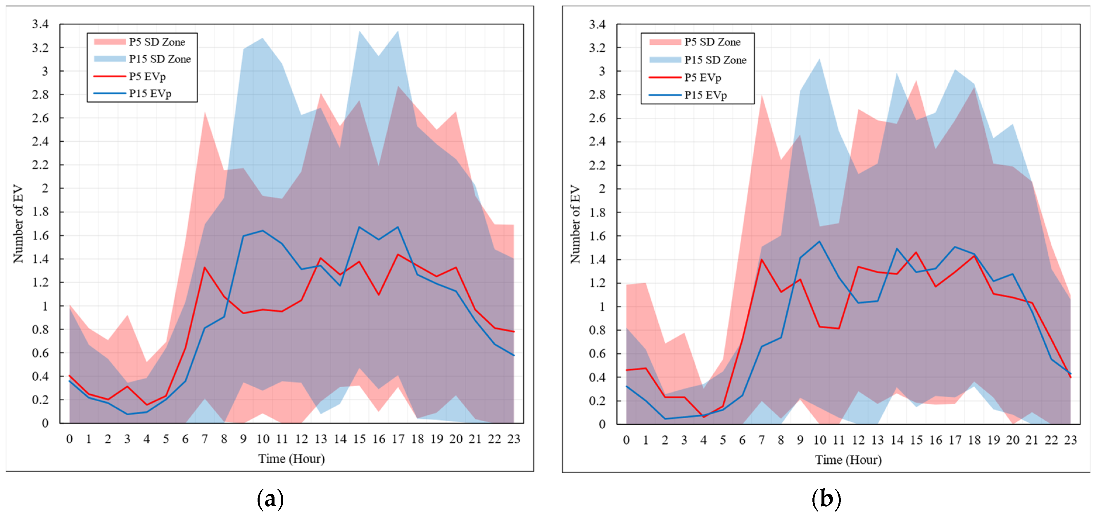
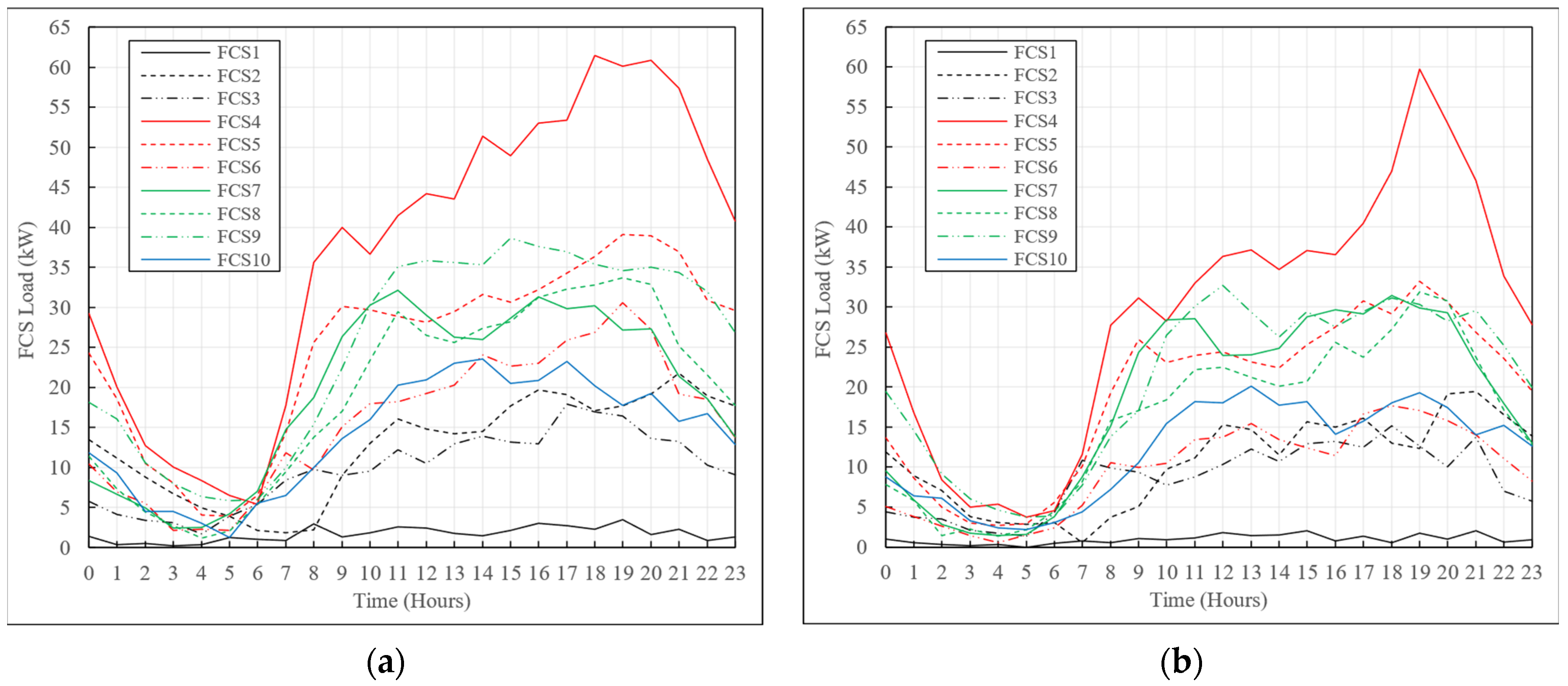
4.2. Base Case Results
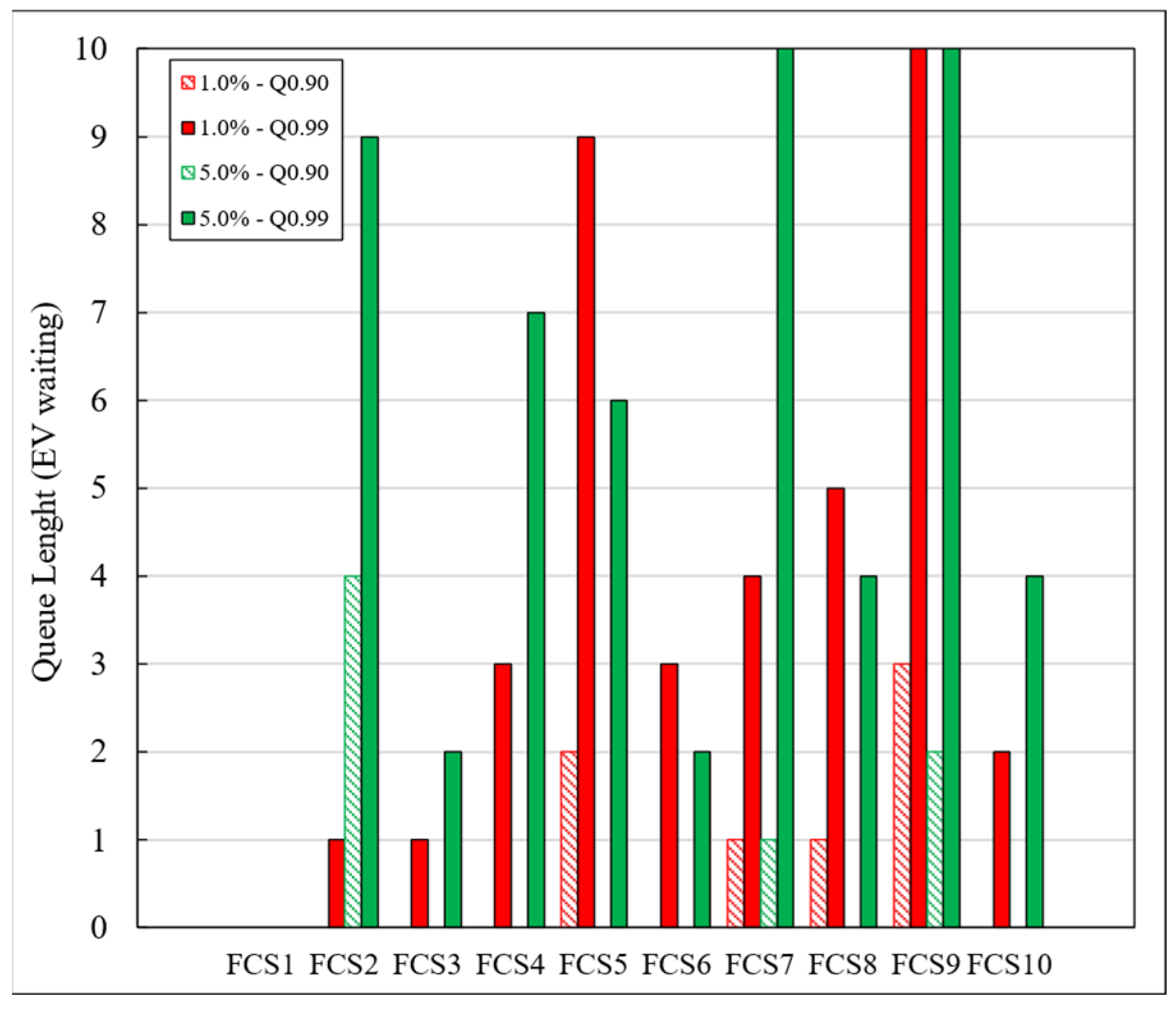
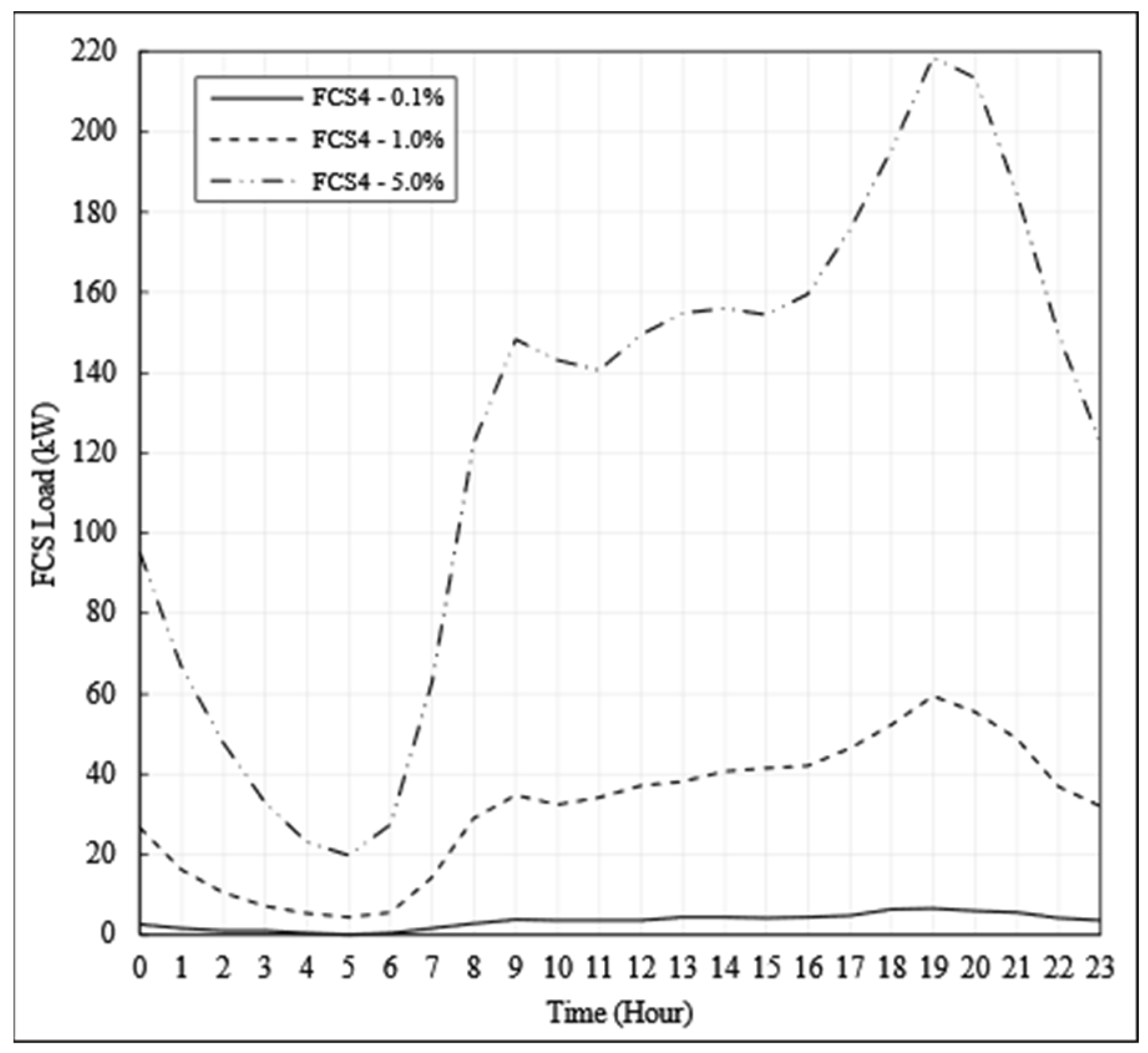
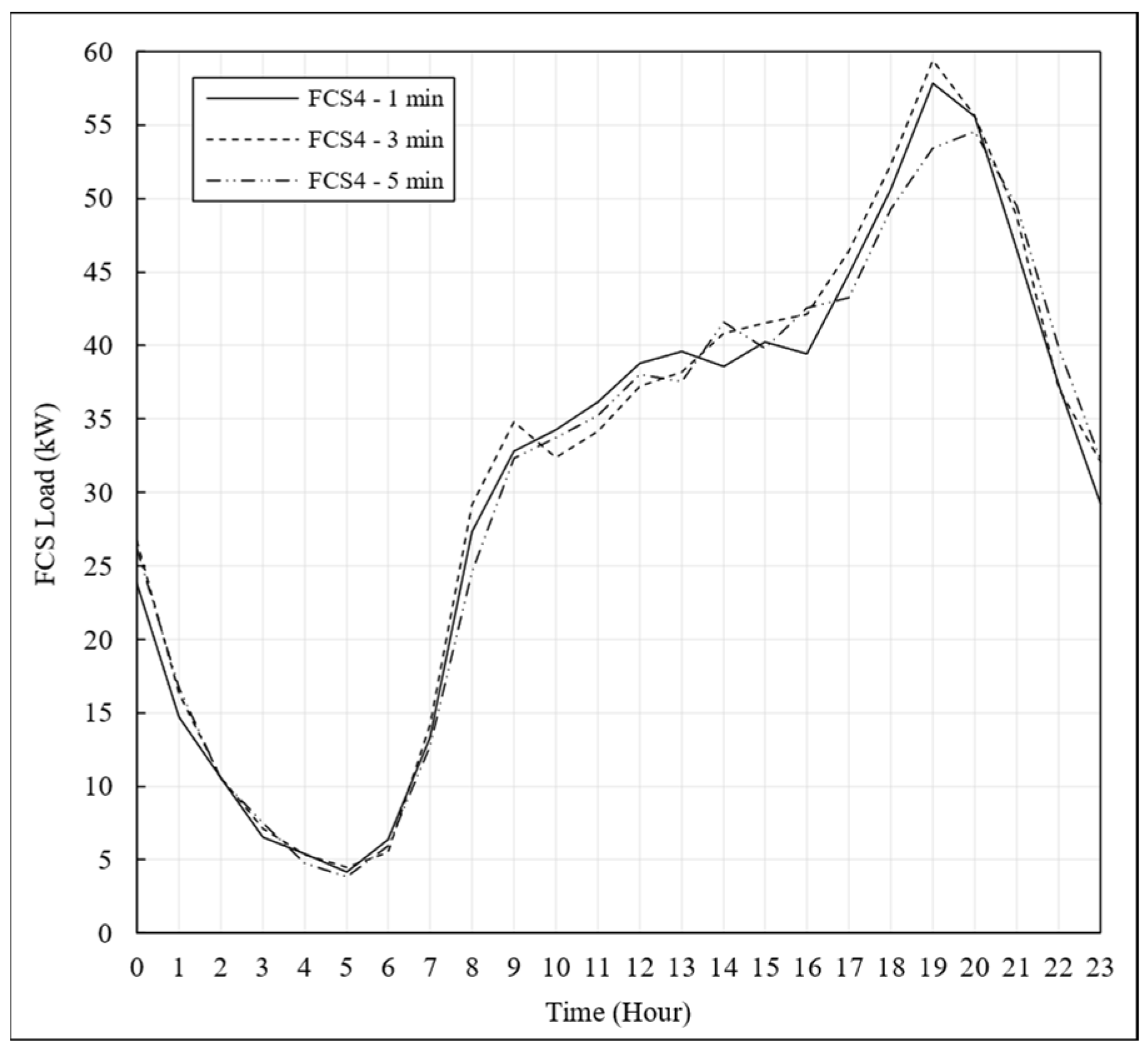
4.3. Sensibilities Analysis
5. Conclusions
5.1. Impact on EV Infrastructure
5.2. Impact on EV User Experience and Market
5.3. Impact on Policies
Author Contributions
Funding
Data Availability Statement
Conflicts of Interest
References
- Das, H.S.; Rahman, M.M.; Li, S.; Tan, C.W. Electric Vehicles Standards, Charging Infrastructure, and Impact on Grid Integration: A Technological Review. Renew. Sustain. Energy Rev. 2020, 120, 109618. [Google Scholar] [CrossRef]
- IEA. Global EV Outlook 2022; IEA Publications: Paris, France, 2022. [Google Scholar]
- Hardman, S.; Jenn, A.; Tal, G.; Axsen, J.; Beard, G.; Daina, N.; Figenbaum, E.; Jakobsson, N.; Jochem, P.; Kinnear, N.; et al. A Review of Consumer Preferences of and Interactions with Electric Vehicle Charging Infrastructure. Transp. Res. Part D Transp. Environ. 2018, 62, 508–523. [Google Scholar] [CrossRef]
- Dong, X.; Mu, Y.; Jia, H.; Wu, J.; Yu, X. Planning of Fast EV Charging Stations on a Round Freeway. IEEE Trans. Sustain. Energy 2016, 7, 1452–1461. [Google Scholar] [CrossRef]
- Colmenar-Santos, A.; de Palacio, C.; Borge-Diez, D.; Monzón-Alejandro, O. Planning Minimum Interurban Fast Charging Infrastructure for Electric Vehicles: Methodology and Application to Spain. Energies 2014, 7, 1207–1229. [Google Scholar] [CrossRef]
- Luo, C.; Huang, Y.-F.; Gupta, V. Stochastic Dynamic Pricing for EV Charging Stations With Renewable Integration and Energy Storage. IEEE Trans. Smart Grid 2018, 9, 1494–1505. [Google Scholar] [CrossRef]
- Motoaki, Y.; Shirk, M.G. Consumer Behavioral Adaption in EV Fast Charging through Pricing. Energy Policy 2017, 108, 178–183. [Google Scholar] [CrossRef]
- Burnham, A.; Dufek, E.J.; Stephens, T.; Francfort, J.; Michelbacher, C.; Carlson, R.B.; Zhang, J.; Vijayagopal, R.; Dias, F.; Mohanpurkar, M.; et al. Enabling Fast Charging—Infrastructure and Economic Considerations. J. Power Sources 2017, 367, 237–249. [Google Scholar] [CrossRef]
- Gusrialdi, A.; Qu, Z.; Simaan, M.A. Scheduling and Cooperative Control of Electric Vehicles’ Charging at Highway Service Stations. In Proceedings of the 53rd IEEE Conference on Decision and Control, Los Angeles, CA, USA, 15–17 December 2014; IEEE: New York, NY, USA, 2014; pp. 6465–6471. [Google Scholar]
- Zarazua de Rubens, G.; Noel, L.; Kester, J.; Sovacool, B.K. The Market Case for Electric Mobility: Investigating Electric Vehicle Business Models for Mass Adoption. Energy 2020, 194, 116841. [Google Scholar] [CrossRef]
- Napoli, G.; Polimeni, A.; Micari, S.; Andaloro, L.; Antonucci, V. Optimal Allocation of Electric Vehicle Charging Stations in a Highway Network: Part 1. Methodology and Test Application. J. Energy Storage 2020, 27, 101102. [Google Scholar] [CrossRef]
- Dong, X.; Yuan, K.; Song, Y.; Mu, Y.; Jia, H. A Load Forecast Method for Fast Charging Stations of Electric Vehicles on the Freeway Considering the Information Interaction. Energy Procedia 2017, 142, 2171–2176. [Google Scholar] [CrossRef]
- Korolko, N.; Sahinoglu, Z.; Nikovski, D. Modeling and Forecasting Self-Similar Power Load Due to EV Fast Chargers. IEEE Trans. Smart Grid 2016, 7, 1620–1629. [Google Scholar] [CrossRef]
- Arias, M.B.; Bae, S. Electric Vehicle Charging Demand Forecasting Model Based on Big Data Technologies. Appl. Energy 2016, 183, 327–339. [Google Scholar] [CrossRef]
- Savari, G.F.; Krishnasamy, V.; Sathik, J.; Ali, Z.M.; Abdel Aleem, S.H.E. Internet of Things Based Real-Time Electric Vehicle Load Forecasting and Charging Station Recommendation. ISA Trans. 2020, 97, 431–447. [Google Scholar] [CrossRef] [PubMed]
- Daneshzand, F.; Coker, P.; Potter, B.; Smith, S. EV smart charging: How tariff selection influences grid stress and carbon reduction. Appl. Energy 2023, 348, 121482. [Google Scholar] [CrossRef]
- Silva, L.; Abaide, A.; Sausen, J.; Paixão, J.; Correa, C. Proposal of a Load Curve modeling applied to Highway EV Fast Charging Stations. In Proceedings of the 2021 56th International Universities Power Engineering Conference (UPEC), Middlesbrough, UK, 31 August–3 September 2021; IEEE: New York, NY, USA, 2021. [Google Scholar] [CrossRef]
- Domínguez-Navarro, J.A.; Dufo-López, R.; Yusta-Loyo, J.M.; Artal-Sevil, J.S.; Bernal-Agustín, J.L. Design of an Electric Vehicle Fast-Charging Station with Integration of Renewable Energy and Storage Systems. Int. J. Electr. Power Energy Syst. 2019, 105, 46–58. [Google Scholar] [CrossRef]
- Bae, S.; Kwasinski, A. Spatial and Temporal Model of Electric Vehicle Charging Demand. IEEE Trans. Smart Grid 2012, 3, 394–403. [Google Scholar] [CrossRef]
- del Razo, V.; Jacobsen, H.-A. Smart Charging Schedules for Highway Travel With Electric Vehicles. IEEE Trans. Transp. Electrif. 2016, 2, 160–173. [Google Scholar] [CrossRef]
- Yuan, K.; Song, Y.; Shao, Y.; Sun, C.; Wu, Z. A Charging Strategy with the Price Stimulus Considering the Queue of Charging Station and EV Fast Charging Demand. Energy Procedia 2018, 145, 400–405. [Google Scholar] [CrossRef]
- Paatero, J.V.; Lund, P.D. A Model for Generating Household Electricity Load Profiles. Int. J. Energy Res. 2006, 30, 273–290. [Google Scholar] [CrossRef]
- Armstrong, M.M.; Swinton, M.C.; Ribberink, H.; Beausoleil-Morrison, I.; Millette, J. Synthetically Derived Profiles for Representing Occupant-Driven Electric Loads in Canadian Housing. J. Build. Perform. Simul. 2009, 2, 15–30. [Google Scholar] [CrossRef]
- Quiros-Tortos, J.; Ochoa, L.F.; Lees, B. A Statistical Analysis of EV Charging Behavior in the UK. In Proceedings of the 2015 IEEE PES Innovative Smart Grid Technologies Latin America (ISGT LATAM), Montevideo, Uruguay, 5–7 October 2015; IEEE: New York, NY, USA, 2015; pp. 445–449. [Google Scholar]
- Hardinghaus, M.; Blümel, H.; Seidel, C. Charging Infrastructure Implementation for EVs—The Case of Berlin. Transp. Res. Procedia 2016, 14, 2594–2603. [Google Scholar] [CrossRef]
- Langbroek, J.H.M.; Franklin, J.P.; Susilo, Y.O. When Do You Charge Your Electric Vehicle? A Stated Adaptation Approach. Energy Policy 2017, 108, 565–573. [Google Scholar] [CrossRef]
- Gnann, T.; Funke, S.; Jakobsson, N.; Plötz, P.; Sprei, F.; Bennehag, A. Fast Charging Infrastructure for Electric Vehicles: Today’s Situation and Future Needs. Transp. Res. Part D Transp. Environ. 2018, 62, 314–329. [Google Scholar] [CrossRef]
- Rominger, J.; Farkas, C. Public Charging Infrastructure in Japan—A Stochastic Modelling Analysis. Int. J. Electr. Power Energy Syst. 2017, 90, 134–146. [Google Scholar] [CrossRef]
- DNIT Plano Nacional de Contagem de Tráfego. Available online: http://servicos.dnit.gov.br/dadospnct/ContagemContinua (accessed on 25 March 2022).


| Force between 2 points on the highway | State-of-Charge | ||
| Interactable variable | Anxiety range | ||
| Maximum MCS scenarios | |||
| on the highway | Maximum number of interactions without result upgrades | ||
| MCS early stop accuracy index | |||
| (km/h) | |||
| Origin self-index | |||
| Destination self-index | between two highway points | ||
| Origin matrix | |||
| Destination matrix | Matrix of total EV leaving the highway | ||
| Empirical parameter for a better fit of OD matrix elements | permanently | ||
| Point index | Matrix of total EV entering the highway | ||
| Maximum number of highway points | permanently | ||
| Subpoint index | Matrix of net EV number in the highway points | ||
| Maximum number of highways subpoints | |||
| (km) | Time step index | ||
| (km) | Time step length (minutes) | ||
| (km) | Simulation time horizon | ||
| (km) | Simulation horizon (hours) | ||
| charging duration (minutes) | in one highway sense | ||
| Charger Power (kW) | |||
| Charger index | |||
| Total MCS simulated scenarios | Total charging event duration | ||
| Flexibility index for charging events in next FCSs | Time between two consecutive charging events | ||
| Entrance probability of one FCS | |||
| Charging duration frequency distribution | |||
| EV type frequency distribution |
| Point | Type | Population (×1000) | Dist. Next Point (km) | Dist. Next FCS (km) | Average Speed (km/h) |
|---|---|---|---|---|---|
| P1 | City | 50.00 | 5 | - | 80 |
| P2 | FCS | - | 40 | 105 | 80 |
| P3 | City | 18.18 | 65 | - | 80 |
| P4 | FCS | - | 20 | 25 | 80 |
| P5 | City | 555.10 | 5 | - | 100 |
| P6 | FCS | - | 58 | 100 | 100 |
| P7 | City | 35.00 | 37 | - | 100 |
| P8 | City | 7.28 | 5 | - | 100 |
| P9 | FCS | - | 25 | 70 | 100 |
| P10 | City | 47.06 | 35 | - | 100 |
| P11 | City | 17.33 | 10 | - | 100 |
| P12 | FCS | - | 35 | 73 | 100 |
| P13 | City | 12.57 | 38 | - | 100 |
| P14 | FCS | - | 5 | 10 | 100 |
| P15 | City | 4319.86 | 5 | - | 100 |
| P16 | FCS | - | 106 | 106 | 100 |
| P17 | FCS | - | 5 | 40 | 100 |
| P18 | City | 43.17 | 25 | - | 100 |
| P19 | City | 135.39 1/257.71 2 | 10 | - | 100 |
| P20 | FCS | - | 10 | 80 | 100 |
| P21 | City | 66.26 1/151.48 2 | 70 | - | 100 |
| P22 | FCS | - | 10 | 10 | 100 |
| P23 | City | 39.87 1/63.64 2 | - | - | 100 |
| Point | Direct Sense | Reverse Sense | ||
|---|---|---|---|---|
| Veh. Average | Veh. Max | Veh. Average | Veh. Max | |
| P1 | 29 | 159 | - | - |
| P3 | 10 | 56 | 0 | 6 |
| P5 | 390 | 1266 | 35 | 193 |
| P7 | 23 | 79 | 3 | 11 |
| P8 | 4 | 16 | 0 | 2 |
| P10 | 32 | 105 | 4 | 15 |
| P11 | 11 | 38 | 1 | 5 |
| P13 | 8 | 28 | 0 | 4 |
| P15 | 428 | 3252 | 368 | 1417 |
| P18 | 4 | 29 | 40 | 390 |
| P19 | 19 | 175 | 151 | 1226 |
| P21 | 10 | 103 | 79 | 713 |
| P23 | - | - | 272 | 1492 |
| EV | Units 1 | EV Fleet Share | Range (km) | Bat. Cap. (kWh) |
|---|---|---|---|---|
| Volvo XC40 RP | 881 | 27% | 300 2 | 67 |
| Porsche Taycan | 495 | 15% | 385 2 | 71 |
| Audi E-tron | 459 | 14% | 330 2 | 86.5 |
| Renault Zoe | 316 | 10% | 285 2 | 52 |
| Fiat 500e | 313 | 9% | 215 2 | 37.3 |
| Chevrolet Bolt | 245 | 7% | 300 3 | 66 |
| Jaguar I-PACE | 234 | 7% | 345 2 | 84.7 |
| JAC E-JS4 | 132 | 4% | 280 3 | 55 |
| Arrizo 5E | 130 | 4% | 200 3 | 53.5 |
| Model S | 61 | 2% | 555 2 | 95 |
| Model 3 | 57 | 2% | 360 2 | 57.5 |
| FCS | 2019 FCS | Max. Cons. | Min. Cons. | ||
|---|---|---|---|---|---|
| Energy (MWh) | Month | MWh | Veh. Max | MWh | |
| FCS1 | 10.65 | January | 1.48 | June | 0.54 |
| FCS2 | 97.09 | January | 9.87 | April | 6.77 |
| FCS3 | 76.19 | January | 8.78 | May | 4.89 |
| FCS4 | 274.58 | January | 29.33 | June | 20.13 |
| FCS5 | 185.82 | January | 20.99 | April | 13.22 |
| FCS6 | 100.20 | January | 12.84 | June | 5.91 |
| FCS7 | 162.62 | June | 14.82 | May | 12.02 |
| FCS8 | 147.33 | January | 15.17 | September | 10.65 |
| FCS9 | 197.05 | December | 19.09 | September | 13.50 |
| FCS10 | 104.72 | January | 11.05 | November | 7.36 |
| Station | Point | 0.10% EV MS | 1.00% EV MS | 5.00% EV MS |
|---|---|---|---|---|
| FCS1 | P2 | 1 (60 kW) | 1 (60 kW) | 1 (60 kW) |
| FCS2 | P4 | 1 (60 kW) | 1 (60 kW) | 1 (60 kW) |
| FCS3 | P6 | 1 (60 kW) | 1 (60 kW) | 3 (180 kW) |
| FCS4 | P9 | 1 (60 kW) | 2 (120 kW) | 6 (360 kW) |
| FCS5 | P12 | 1 (60 kW) | 1 (60 kW) | 5 (300 kW) |
| FCS6 | P14 | 1 (60 kW) | 1 (60 kW) | 4 (240 kW) |
| FCS7 | P16 | 1 (60 kW) | 1 (60 kW) | 4 (240 kW) |
| FCS8 | P17 | 1 (60 kW) | 1 (60 kW) | 5 (300 kW) |
| FCS9 | P20 | 1 (60 kW) | 1 (60 kW) | 4 (240 kW) |
| FCS10 | P22 | 1 (60 kW) | 1 (60 kW) | 3 (180 kW) |
| Q0.85 | Q0.90 | Q0.95 | Q0.99 | |
|---|---|---|---|---|
| 1 min | 0 | 0 | 1 | 2 |
| 3 min | 0 | 0 | 1 | 3 |
| 5 min | 0 | 1 | 2 | 5 |
| Aspect | Parameter | Base Case | Pessimist Case |
|---|---|---|---|
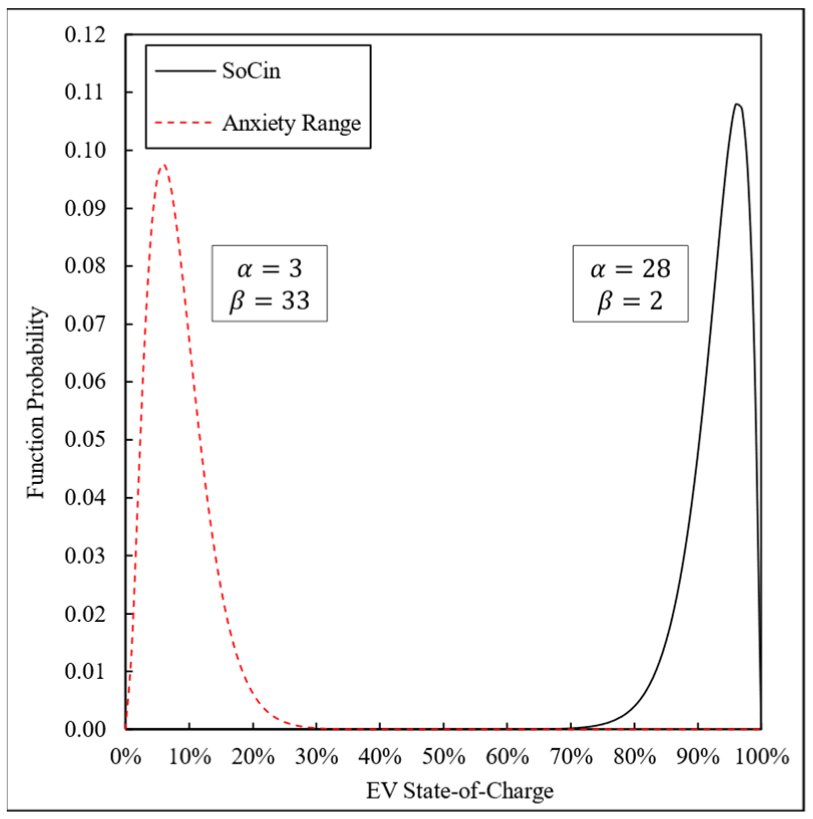
| SoC | 28 | 25 | |
| 2 | 5 | ||
| 0.96 | 0.85 | ||
| AR | 3 | 5 | |
| 33 | 25 | ||
| 0.06 | 0.15 | ||
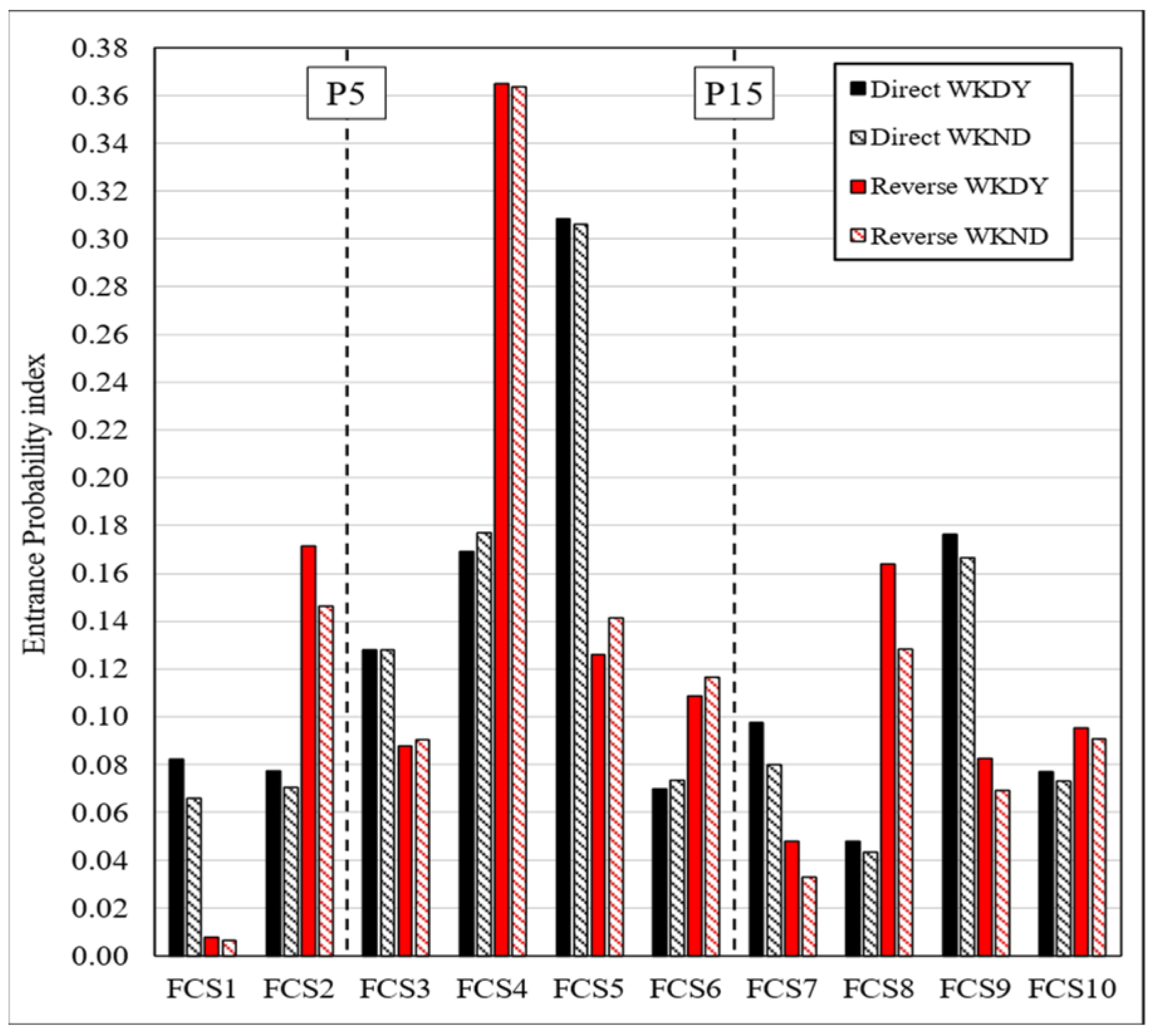
| FCS Entry Probability | Direct WKDY | 0.17 | 0.36 |
| Direct WKND | 0.18 | 0.36 | |
| Reverse WKDY | 0.37 | 0.76 | |
| Reverse WKND | 0.36 | 0.77 | |
| Energy | 2019 FCS Energy | 274.58 MWh | 496.29 MWh |
| Queue Length | Q0.85 | 0 | 3 |
| Q0.90 | 0 | 5 | |
| Q0.95 | 1 | 8 | |
| Q0.99 | 3 | 15 |
Disclaimer/Publisher’s Note: The statements, opinions and data contained in all publications are solely those of the individual author(s) and contributor(s) and not of MDPI and/or the editor(s). MDPI and/or the editor(s) disclaim responsibility for any injury to people or property resulting from any ideas, methods, instructions or products referred to in the content. |
© 2024 by the authors. Licensee MDPI, Basel, Switzerland. This article is an open access article distributed under the terms and conditions of the Creative Commons Attribution (CC BY) license (https://creativecommons.org/licenses/by/4.0/).
Share and Cite
Silva, L.N.F.d.; Capeletti, M.B.; Abaide, A.d.R.; Pfitscher, L.L. A Stochastic Methodology for EV Fast-Charging Load Curve Estimation Considering the Highway Traffic and User Behavior. Energies 2024, 17, 1764. https://doi.org/10.3390/en17071764
Silva LNFd, Capeletti MB, Abaide AdR, Pfitscher LL. A Stochastic Methodology for EV Fast-Charging Load Curve Estimation Considering the Highway Traffic and User Behavior. Energies. 2024; 17(7):1764. https://doi.org/10.3390/en17071764
Chicago/Turabian StyleSilva, Leonardo Nogueira Fontoura da, Marcelo Bruno Capeletti, Alzenira da Rosa Abaide, and Luciano Lopes Pfitscher. 2024. "A Stochastic Methodology for EV Fast-Charging Load Curve Estimation Considering the Highway Traffic and User Behavior" Energies 17, no. 7: 1764. https://doi.org/10.3390/en17071764