Abstract
The premise for formulating effective emission control strategies is to accurately and reasonably evaluate the actual emission level of vehicles. Firstly, the active subspace method is applied to set up a low-dimensional model of the relationship between CO2 emission and multivariate vehicle driving data, in which the vehicle specific power (VSP) is identified as the most significant factor on the CO2 emission factor, followed by speed. Additionally, acceleration and exhaust temperature had the least impact. It is inferred that the changes in data sampling transform the establishment of subspace matrices, affecting the calculation of eigenvector components and the fitting of the final quadratic response surface, so that the emission sensitivity and final fitting accuracy are impressionable by the data distribution form. For the VSP, the best fitting result can be obtained when the VSP conforms to a uniform distribution. Moreover, the Bayesian linear regression method accounts for fitting parameters between the VSP and CO2 emission factor with uncertainties derived from heteroscedastic measurement errors, and the values and distributions of the intercept and slope α and β are obtained. In general, the high-resolution inventory of the carbon emission factor of the tested vehicle is set up via systematically analyzing it, which brings a bright view of data processing in further counting the carbon footprint.
1. Introduction
The transportation sector is the third largest CO2 emission source after power and industry. Carbon emissions from transportation can cause significant harm to the climate and environment [1]. Therefore, how to reduce vehicle exhaust pollution and greenhouse gas emissions has become an undeniable challenge [2]. Roughly, China emitted 35% of the world’s total CO2 emissions in 2023 [3]. Road transportation contributes to 70~80% of the CO2 emissions in the transportation sector of China, which still dominates as one of the largest parts of total carbon emissions [4,5]. An action plan of decarbonizing China’s road transport is becoming among the stated national policies [6]; meanwhile, the technology roadmap for energy saving and new energy vehicles is being undertaken by many researchers and institutes, with the aim to achieve carbon neutrality by 2060.
How to accurately and reasonably evaluate the actual emission level of vehicles is a prerequisite for formulating effective emission control strategies. Many scholars have conducted research on this issue. When characterizing the emission characteristics of different operating conditions, instantaneous operating parameters such as speed [7,8], acceleration [9,10], fuel consumption [11,12], and driving distance [13] are used while the vehicle specific power (VSP) is a newly proposed alternative parameter in correlation with speed and acceleration. Jimenez et al. [14] found that the VSP could capture the majority of the dependence of light vehicle emissions on driving conditions when combined with traffic flow data, thus improving the accuracy of the predicted emissions. Song et al. [15] compared the estimated fuel consumption with actual data and demonstrated that the VSP bin distribution model is reliable and accurate in estimating fuel consumption. When the real-time speed data are available, the speed-specific VSP bin distribution model may help monitor dynamic transportation, to facilitate quantifying the relationship between VSP distributions and vehicle fuel consumption or emissions. Forcetto et al. [16] applied the VSP as an additional parameter for improving the evaluation of the vehicle dynamics, which can add a better comprehension of the real drive emission (RDE) dynamic, complementing the regulatory parameters. By combining fuel consumption rates with VSP distributions, Zhang, L. et al. [17] proposed an improved method for evaluating eco-driving behavior depending on the VSP distribution at a specific speed, providing a potential way to evaluate fuel consumption and emission combined with traffic conditions.
Vehicle CO2 emission is typically influenced by a combination of multiple factors, so it is necessary to reveal the impacts of simultaneous multi-factor variables on emission factors, in order to summarize the methods for constructing a high-resolution database of the carbon emission factor. At present, existing multi-factor variable analysis models, such as COPERT [18,19], MOBILE [20,21], IVE [22], etc., are all based on static factors such as vehicle type, vehicle mileage, fuel quality, and fuel volatility to study the vehicle emission factors of motor vehicles. The traditional one-at-a-time (OAT) sensitivity analysis applied in the sensitivity analysis can only predict the relative sensitivity of a single input parameter at a time, so that it precludes the synergistic effects between multiple input parameters. A multivariate analysis is able to reflect the combined effects of multiple variables on output, which displays a more accurate and flexible performance than an OAT sensitivity analysis. However, a multi-factor analysis of emission factors based on dynamic driving conditions is rarely reported.
The active subspace (AS) is an emerging dimensionality reduction method for multivariate analysis, which can obtain the low-dimensional structure of the multivariate function by transforming the high-dimensional space [23,24]. At the same time, the component values of the active direction vector can provide global sensitivity information of the target quantity relative to the input parameters [25]. In the field of engineering, the active subspace method has been applied in sensitivity analysis studies of turbomachinery [26,27] and combustion [28,29,30], but, up to now, few reports of AS application in transportation emissions analysis had been presented.
Moreover, as the data size increases, the uncertainties driven by the error distribution from the sampling data play an important role in the accounting accuracy of carbon emissions under varied transportation scenarios. Thus, uncertainty quantification is necessary when formulating emission factor models based on real-driving cycles.
Bayesian inference methods have been used widely for model calibration and uncertainty analysis [31,32]. The goal of the Bayesian regression method is to characterize the parameter distribution consistent with the given experimental dataset, instead of finding the best fit for regression model parameters [33,34]. Li et al. [35] used Bayesian approaches to explicitly accommodate the uncertainty of the model predictions. Mudgal, A. et al. [36] modeled the speed profiles of drivers by using a Bayesian inference methodology, and then estimated the vehicular emissions using past experimental data. Martin et al. [37] presented a new Bayesian methodology called the Cambridge Automotive Research Modelling Application (CARma), which was able to categorize the sources of uncertainty and calibrate uncertain parameters to present the results as probability distribution functions.
The active subspace method and Bayesian linear fitting method are used in this study to combine multivariate analysis with uncertainty analysis, explore the sensitivity of vehicle emissions to operating parameters, and improve the accuracy of emission prediction by considering the distribution of operating points. This method comprehensively studies the impact of vehicle driving parameters on emission factors, laying the foundation for constructing a high-resolution database of the carbon emission factor. The study is structured as follows: In Section 2, the methodologies of this study are introduced, including the data processing and the principles of data analysis methods, such as multivariate analysis and uncertainty analysis. Then, Section 3 describes the details analysis of the sensitivity and the uncertainty of the carbon emission factor. Finally, some concluding remarks are given in Section 4.
2. Materials and Methods
2.1. Data Source
In China, light gasoline vehicles account for a large proportion of road traffic. Meanwhile, China has fully implemented the national VI motor vehicle emission standards. Therefore, in this study, the multi-purpose gasoline passenger vehicle that meets the national VI motor vehicle emission standards was chosen. The source of data used in this study is the RDE test conducted by China Automotive Engineering Research Institute Co., Ltd. (Chongqing, China).
The RDE test was conducted once and employed by using on-board emission measurement system OBS-ONE GS Unit from Japan’s HORIBA company to measure the vehicle’s emissions per second. The test route is shown in Figure 1. The test route is located in Chongqing, China. The total length of this route is 82.096 km, and the maximum altitude and minimum altitude are 499.4 m and 240.9 m, respectively. The test data are divided into three working conditions based on the vehicle’s driving speed, urban (v ≤ 60 km/h), suburban (60 km/h < v ≤ 90 km/h), and highway (v > 90 km/h), as shown in Figure 2, and the distribution of driving conditions is shown in Table 1.
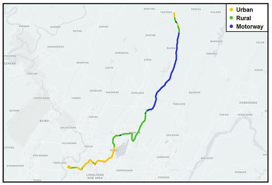
Figure 1.
Testing route.
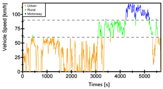
Figure 2.
The speed structure of vehicle driving.

Table 1.
Distribution of vehicle driving conditions.
2.2. VSP Binning Method
VSP is a dynamic proxy variable of the vehicle with vector nature, defined as the power output per unit mass of motor vehicle towed by the engine (kw/t) or m2/s3 [14]. For light gasoline vehicles, the formula for VSP is computed as [38]:
where v is the driving speed of the tested vehicle in a unit of m/s, and a is the driving acceleration of the tested vehicle in a unit of m/s2.
The values of VSP can be one-to-one corresponded and classified with cluster bins, thus using the overall VSP distribution as a function of average vehicle speed for statistical analysis. Since there is a certain degree of discreteness in RDE data, this study conducted cluster analysis on VSP [38], when VSP bin = k, and . The data are mainly concentrated in , accounting for 96.93%. Therefore, this study mainly focuses on the data in this range, and the VSP bin distribution is shown in Figure 3.
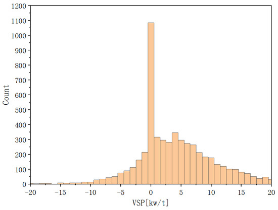
Figure 3.
VSP bin distribution of the RDE data.
The traffic carbon emission factor generally refers to the carbon emissions generated per unit workload, in order to evaluate carbon emission efficiency. This study applies the speed-specific CO2 emission factor based on driving distance to characterize the mass of CO2 emitted by motor vehicles per unit distance (g/km), which can be obtained by Equation (2):
where EFk, ERk, and vk, respectively, represent the CO2 emission factor (g/km), CO2 emission rate (g/s), and driving speed (km/h) of the tested vehicle when VSP bin = k.
2.3. Active Subspace Method
The active subspace is a type of low-dimensional structure in a function of several variables. It can achieve dimensionality reduction through transformations in high-dimensional spaces, which essentially involves important directions with higher sensitivity in high-dimensional spaces through linear space transformations. In the present study, a one-dimensional active subspace is observed to figure out the key contributors to the variability in the emission factor response. The input–output response diagram is approximated by a linear model. This method is applicable when both conditions are satisfied that the activity subspace is one-dimensional and the relationship between the quantity of interest and its input parameters is approximately monotonic. The sufficient summary plot shows the relationship between the linear combination of the quantity of interest and input parameters (i.e., active variables), with the weights of the linear combination being the components of the normalized gradient of the linear model. Each point on the plot represents a set of inputs and corresponding outputs of the model. The specific flowchart of performing the active subspace method for sensitivity analysis is shown in Figure 4. In the current study, speed, acceleration, VSP, CO2 emission rate, and exhaust temperature are selected as input variables, and corresponding CO2 emission factor as the quantity of interest.
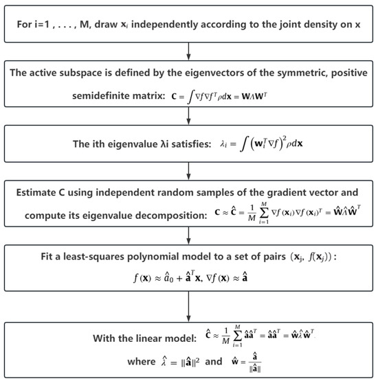
Figure 4.
Workflow of active subspace method.
The active subspace is defined by the eigenvectors of a symmetric positive semidefinite matrix:
where W is the orthogonal matrix of the eigenvector, and Λ is the diagonal matrix of non-negative eigenvalues arranged in descending order.
To estimate the eigenvectors and eigenvalues, independent random samples of gradient vector are used to estimate C and calculate its eigenvalue decomposition [39]:
where xi are based on drawing randomly and independently.
In this study, the gradient of polynomial approximation is worked out and the least-squares polynomial model is fitted to a pair of . When the polynomial approximation is a linear function of x, the calculation amount of decreases sharply. The gradient of the global linear model is constant for all x:
Thus, can be expressed as:
where is the normalized gradient of the linear model. In a linear model, only one-dimensional active subspace can be identified.
2.4. Bayesian Linear Regression
Bayesian linear regression is a method that uses probability distribution rather than point estimation to construct linear regression. The response variable y is not a single value to be estimated, but a probability distribution assumed to be extracted from a normal distribution. The posterior probability distribution of model parameters P(β|y,X) is conditional on the inputs and output of the training, as calculated in Equation (8):
which is equal to the likelihood P(y|β,X) multiplied by the prior probability distribution P(β|X) of the parameter β of the given input and divided by the normalization constant.
In this study, the data with heteroscedastic measurement errors (errors with different variances) in both variables are regression-fitted through Bayesian theory. It is assumed that the independent variable and the dependent variable follow a Gaussian distribution, and that is a random vector of n data points extracted from a certain probability distribution [40,41]. According to the usual additive model, the dependent variable depends on :
where is a random variable which represents the intrinsic scatter in i about the regression relationship and are the regression coefficients. The mean of is assumed to be zero and the variance is constant. The values (x, y) measured with errors are observed instead of the actual values of (, ). The measured values are assumed to be related to the actual values as:
where and are, respectively, the random measurement errors on and , which are normally distributed with known variances and and covariance . The variances and covariance are assumed to be the same for each data point in this study.
Due to the complexity of parameter distribution, the Markov chain Monte Carlo (MCMC) method is introduced to conduct efficient sampling and promote the final convergence to the target distribution. By using MCMC, the mathematical expectation of the posterior distribution inferred by Bayesian inference is obtained as the estimated value of the parameter.
3. Results and Discussion
3.1. Multivariate Sensitivity Analysis of CO2 Emission Factor
The components of the eigenvector are plotted in Figure 5; the single-column active variable weights quantify the sensitivity of the output to input parameters. The larger the weights, the greater the changes in the CO2 emission factor caused by the corresponding parameters. The CO2 emission rate (CO2/[g/s]) is definitely the most influential input parameter for the CO2 emission factor, and the VSP (vsp/[kw/t]) and speed (v/[km/h]) are coming next, with the VSP having a greater weight than speed. In addition, the influence of acceleration (a/[m/s2]) and exhaust temperature (ExhaustTemp/[degC]) is minimal.
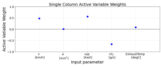
Figure 5.
Input parameter weights calculated using all operating points.
The symbol of the input parameter weight can represent the positive and negative ratio relationship between the output parameter and input parameters. Meanwhile, the trend of the change can also be quantitatively described by the quadratic response surface curves and the influence of the eigenvector components on the activity variables (as seen in Figure 6). When all other input parameters suppose fixed values, the CO2 emission factor decreased by 3.333% when v is increased from 5 to 10, and continually decreased by 3.330% when v reached 15. In general, the CO2 emission factor will increase with a decrease in speed. This result may be caused by the definition of the emission factor, which is based on the driving distance (Equation (2)). When the speed decreases, decreases, and the amplitude of the change is much smaller than , hence resulting in an increase in .
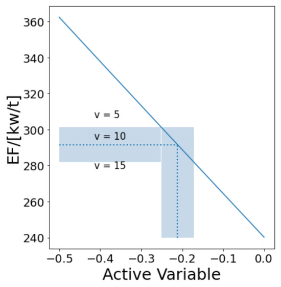
Figure 6.
Estimation of output change with respect to input parameter values.
3.2. Inference of CO2 Emission Factor by Bayesian Regression
The relationship of the CO2 emission factor with the VSP is plotted in Figure 7, with the error bars indicating a 2σ- uncertainty of the data points. The test data are first fitted by the method of ordinary least squares without considering errors, and the fitting function is:
where is the value of the CO2 emission factor, and is the VSP bin value.
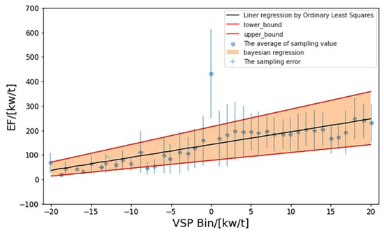
Figure 7.
Regression results for VSP and CO2 emission factor.
The test data are not a fixed value but a distribution within a certain range; the CO2 emission factor should also be taken within a certain range. When considering sampling errors, the uncertainty of the CO2 emission factor is plotted within the shaded area bounded by the upper and lower 95% confidence interval (95% CI) (in Figure 7). Meanwhile, the posterior probability distributions of parameters α and β are shown in Figure 8, as well as MCMC trace-plotting the samples of α and β under the Bayesian framework. The mean posterior distribution of α is 146.5362, while the mean posterior distribution of β is 5.1986. The progressions of the samples plotted in the trajectories of α and β seem to converge well without significant drift.
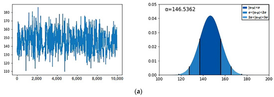
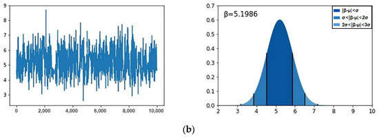
Figure 8.
Tracing plots and posterior probability distribution of parameter by MCMC under Bayesian inference: (a) tracing plots and posterior probability distribution of parameter α by MCMC; (b) tracing plots and posterior probability distribution of parameter by MCMC.
For the surge of the CO2 emission factor when VSP bin = 0 (Figure 7), the reason may be related to the lower vehicle speed. The CO2 emission factor increases with the decrease in vehicle driving speed [42], and approximately 86.67% of the ultra-low speed operating points (v < 10 km/h) are accumulated in the VSP bin = 0 cluster. Meanwhile, the nosedive in vehicle driving speed in the range of VSP bin = 0 may result in sustained carbon dioxide emissions without the mileage being increased, causing a rising change shape in the CO2 emission factor.
3.3. The Influence of Distribution Functions on Multivariate Analysis
Since the surge of the CO2 emission factor when VSP bin = 0 in Section 3.2, only the cases with the VSP bin not being equal to zero are considered in this section, to mitigate the accounting uncertainties. The VSP distribution is determined to be approximately the Rayleigh distribution using the marginal distribution plot and Q–Q plot (Figure 9), with the corresponding p-value being less than 0.05. It can be seen from Figure 9a that, when VSP > 5 and VSP < −5, the marginal distribution of the VSP is in good agreement with the Rayleigh distribution; however, when −5 < VSP < 5, there is a certain deviation. For the Q–Q plot (Figure 9b), the quantile of the probability distribution of the VSP is basically fit to the Rayleigh distribution.
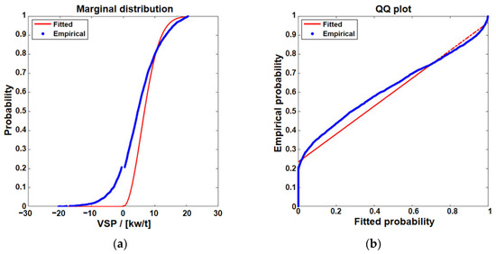
Figure 9.
The marginal distribution of input parameters and Rayleigh distribution and the Quantile–Quantile plots: (a) the marginal distribution; (b) Q–Q plot.
Then, the VSP data are set to the uniform distribution and Rayleigh distribution, respectively, when the distribution functions of other input variables remain unchanged. All input variables are normalized and brought into the active subspace for a sensitivity analysis. The linear combinations of the CO2 emission factor relative to the inputs (i.e., the active variables) exhibit a univariate trend as given in Figure 10, and the relationship between the output and active variables can be represented via a quadratic polynomial:
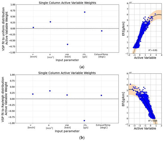
Figure 10.
Input parameter weights and sufficient summary plots calculated when VSP bin = 0 is excluded from data sampling: (a) input parameter weights and sufficient summary plots when VSP fit to uniform distribution; (b) input parameter weights and sufficient summary plots when VSP fit to Rayleigh distribution.
The function g(y) outputs the CO2 emission factor (g/km) where y represents the active variable, which is the weighted sum of the input parameters after scaling.
The CO2 emission can be understood through a powerful information combination of the parameter weights and sufficient summary plots. The positive and negative weights of the input parameters can be used to predict the trend of the changes in the active variables affected by the input parameters, thereby further predicting the trend of the changes in the output parameters. For example, as plotted in Figure 10a, since the VSP index weight is negative for the EF, a greater VSP index decreases the active variable, which results in the decrease in EF. The opposite trend of influence compared to Bayesian fitting is led by the comprehensive influence of other input parameters in multivariate analysis.
It is inferred that the changes in data sampling transform the establishment of subspace matrices, thus affecting the calculation of eigenvector components and the fitting of the final quadratic response surface. As a result, the acceleration and speed, along with the VSP, are combined to become the most influenced factor of the CO2 emission factor when the VSP is sampled according to the Rayleigh distribution. The fitting coefficients C0, C1, and C2 in Equation (13) and the corresponding coefficient of determination (R-squared) values for each of the VSP distribution functions are tabulated in Table 2. Overall, the result of the R-squared from the VSP sampled according to uniform distributions shows a better performance on the goodness of fit. It also suggests that the data shown in Figure 10 are more in line with a quadratic polynomial. Hence, the input parameter distribution function determines the relationship between the combination of inputs and the output of interest to a certain extent.
Table 2.
Summary of quadratic model coefficients.
So far, comprehensive studies on the impact of vehicle driving parameters on emission factors by multivariate sensitivity analysis and uncertainty analysis have been carried out. It is highlighted with high-resolution database processing prepared for the further modelling of the carbon footprint in transportation.
4. Conclusions
In the present study, dynamic vehicle data contributing to traffic carbon emissions are comprehensive studied in the aspects of data sensitivity and uncertainty. The active subspace method can identify which input parameters are the most important through magnitudes of the input parameter weights, while exploring how the combination of inputs is related to the output of interest, without the expense of multiple simulations. It is concluded that the CO2 emission factor is most sensitive to the VSP. The method has great potential to readily derive the relationship between the combination of inputs and outputs in a complex domain without the expense of multiple simulations. And the relationship between the input parameters (i.e., the active variables) and CO2 emission factor is able to be formulated using a quadratic function. Moreover, two domains with varied VSP data distributions are set up to evaluate the sampling diversity on the emission sensitivity. At the same time, a conclusion similar to that in Section 3.3 can be obtained by changing the distribution function of other vehicle operating parameters. But, due to the study only focusing on the RDE data of one light gasoline vehicle, it cannot be guaranteed that the sensitivity analysis of diesel vehicles or non-light gasoline vehicles is consistent with this study.
Concluded from a sensitivity analysis, the relationship between the VSP and CO2 emission factor is explored via the Bayesian linear regression method with the sampling uncertainties considered. The uncertainty of the CO2 emission factor within the upper and lower 95% CI is determined when considering the sampling errors. The uncertainty quantifications for the calibrating parameters α and β are well demonstrated by using the heteroscedasticity measurement errors of both variables. In addition, the reason for the surge of the EF in the VSP bin = 0 cluster is discussed by combining it with the active subspace method. Compared with traditional linear or nonlinear methods, the proposed method takes into account the uncertainty of the parameter distribution and improves the fitting accuracy.
Generally, this article comprehensively studies the impact of vehicle driving parameters on emission factors via multivariate sensitivity analysis and uncertainty quantification analysis. The input parameters that have a significant impact on emission factors are obtained, and the influence of the error distribution and distribution function of the sampled data on the fitting results is explored. On this basis, a new perspective for modelling traffic carbon emission with a high-resolution database is proposed. And it is conducive to improving the accuracy of carbon counting under varied transportation scenarios, laying the foundation for constructing a high-resolution database of the carbon emission factor.
Author Contributions
Conceptualization, F.Z.; methodology, J.C. and F.Z.; validation, J.C.; formal analysis, J.C.; investigation, J.C., H.Y., H.X., Q.L., Z.Z. and H.C.; data curation, H.Y., H.X., Q.L. and Z.Z.; visualization, H.C.; writing—original draft, J.C.; writing—review and editing, F.Z.; funding acquisition, F.Z. and W.Y.; resources, H.Y., H.X., Q.L. and Z.Z.; supervision, F.Z. and W.Y.; project administration, F.Z. and W.Y. All authors have read and agreed to the published version of the manuscript.
Funding
This research was funded by the Open Funds of Chongqing Key Laboratory of Vehicle Emission and Economizing Energy, grant number No. PFJN-09, and the Shandong Provincial Natural Science Foundation, grant number No. 2022HWYQ-061.
Data Availability Statement
Restrictions apply to the availability of these data. Data were obtained from China Automotive Engineering Research Institute Co., Ltd. and are available Feiyang Zhao with the permission of China Automotive Engineering Research Institute Co., Ltd.
Conflicts of Interest
Authors Hao Yu, Haocheng Xu, Qiang Lv and Zongqiang Zhu were employed by the company China Automotive Engineering Research Institute Co., Ltd. The remaining authors declare that the research was conducted in the absence of any commercial or financial relationships that could be construed as a potential conflict of interest.
References
- Hu, G.; Zeng, W.; Yao, R.; Xie, Y.; Liang, S. An integrated assessment system for the carrying capacity of the water environment based on system dynamics. J. Environ. Manag. 2021, 295, 113045. [Google Scholar] [CrossRef] [PubMed]
- Chen, Z.; Li, B.; Jia, S.; Ye, X. Modeling and simulation analysis of vehicle pollution and carbon reduction management model based on system dynamics. Environ. Sci. Pollut. Res. Int. 2023, 30, 14745–14759. [Google Scholar] [CrossRef] [PubMed]
- IEA. CO2 Emissions in 2023; IEA: Paris, France, 2024; Available online: https://www.iea.org/reports/co2-emissions-in-2023 (accessed on 27 April 2023).
- Li, Y.; Dong, H.; Lu, S. Research on application of a hybrid heuristic algorithm in transportation carbon emission. Environ. Sci. Pollut. Res. 2021, 28, 48610–48627. [Google Scholar] [CrossRef] [PubMed]
- Wang, L.; Zhao, Y.; Wang, J.; Liu, J. Regional inequality of total factor CO2 emission performance and its geographical detection in the China’s transportation industry. Environ. Sci. Pollut. Res. Int. 2022, 29, 3037. [Google Scholar] [CrossRef] [PubMed]
- IEA. Energy Technology Perspectives 2015; OECD Publishing: Paris, France, 2015. [Google Scholar]
- Yao, Z.; Cao, H.; Cui, Z.; Wang, Y.; Huang, N. Research on Urban Distribution Routes Considering the Impact of Vehicle Speed on Carbon Emissions. Sustainability 2022, 14, 15827. [Google Scholar] [CrossRef]
- Dong, Y.; Xu, J.; Ni, J. Carbon emission model of vehicles driving at fluctuating speed on highway. Environ. Sci. Pollut. Res. Int. 2023, 30, 18064–18077. [Google Scholar] [CrossRef] [PubMed]
- Rakha, H.; Ahn, K.; Trani, A. Development of VT-Micro model for estimating hot stabilized light duty vehicle and truck emissions. Transportation research. Part D Transp. Environ. 2004, 9, 49–74. [Google Scholar] [CrossRef]
- Kim, W.; Kim, C.; Lee, J.; Kim, J.; Yun, C.; Yook, S. Fine particle emission characteristics of a light-duty diesel vehicle according to vehicle acceleration and road grade. Transp. Res. Part D Transp. Environ. 2017, 53, 428–439. [Google Scholar] [CrossRef]
- Zhao, F.; Liu, F.; Liu, Z.; Hao, H. The correlated impacts of fuel consumption improvements and vehicle electrification on vehicle greenhouse gas emissions in China. J. Clean. Prod. 2019, 207, 702–716. [Google Scholar] [CrossRef]
- Li, X.; Yu, B. Peaking CO2 emissions for China’s urban passenger transport sector. Energy Policy 2019, 133, 110913. [Google Scholar] [CrossRef]
- Pu, X.; Lu, X.; Han, G. An improved optimization algorithm for a multi-depot vehicle routing problem considering carbon emissions. Environ. Sci. Pollut. Res. Int. 2022, 29, 54940–54955. [Google Scholar] [CrossRef] [PubMed]
- Jimenez-Palacios, J.L. Understanding and Quantifying Motor Vehicle Emissions with Vehicle Specific Power and TILDAS Remote Sensing; Massachusetts Institute of Technology: Cambridge, MA, USA, 1999. [Google Scholar]
- Song, G.; Lei, Y. Characteristics of low-speed vehicle-specific power distributions on urban restricted-access roadways in Beijing. Transp. Res. Rec. 2011, 2233, 90–98. [Google Scholar] [CrossRef]
- Forcetto, A.L.S.; de Salvo Junior, O.; Maciel Filho, F.F.; de Fátima Andrade, M.; de Almeida, F.; Flávio Guilherme, V. Improving the assessment of RDE dynamics through vehicle-specific power analysis. Environ. Sci. Pollut. Res. Int. 2022, 29, 59561–59574. [Google Scholar] [CrossRef] [PubMed]
- Zhang, L.; Zhu, Z.; Zhang, Z.; Song, G.; Zhai, Z.; Yu, L. An improved method for evaluating eco-driving behavior based-on speed-specific vehicle-specific power distributions. Transp. Res. Part D Transp. Environ. 2022, 113, 103476. [Google Scholar] [CrossRef]
- Amoatey, P.; Omidvarborna, H.; Baawain, M.S.; Al-Mamun, A. Evaluation of vehicular pollution levels using line source model for hot spots in Muscat, Oman. Environ. Sci. Pollut. Res. Int. 2020, 27, 31184–31201. [Google Scholar] [CrossRef] [PubMed]
- Smit, R.; Awadallah, M.; Bagheri, S.; Surawski, N.C. Real-world emission factors for SUVs using on-board emission testing and geo-computation. Transp. Res. Part D Transp. Environ. 2022, 107, 103286. [Google Scholar] [CrossRef]
- EPA. User’s Guide to Mobile4 (Mobile Source Emission Factor Model); Office of Mobile Sources U.S. Environmental Protection Agency Ann Arbor: Washington, DC, USA, 1989. [Google Scholar]
- EPA. User’s Guide to MOBILE6.1 and MOBILE6.2: Mobile Source Emission Factor Model [CP/OL]. 2008. Available online: http://www.epa.gov/oms/m6.htm,2008/04/05 (accessed on 27 April 2023).
- Khazini, L.; Kalajahi, M.J.; Blond, N. An analysis of emission reduction strategy for light and heavy-duty vehicles pollutions in high spatial–temporal resolution and emission. Environ. Sci. Pollut. Res. Int. 2022, 29, 23419–23435. [Google Scholar] [CrossRef]
- Charles, R.; Crawford. Active Subspaces: Emerging Ideas for Dimension Reduction in Parameter Studies; SIAM: Philadelphia, PA, USA, 2016. [Google Scholar]
- Constantine, P.G.; Emory, M.; Larsson, J.; Iaccarino, G. Exploiting active subspaces to quantify uncertainty in the numerical simulation of the HyShot II scramjet. J. Comput. Phys. 2015, 302, 1–20. [Google Scholar] [CrossRef]
- Constantine, P.G.; Diaz, P. Global sensitivity metrics from active subspaces. Reliab. Eng. Syst. Saf. 2017, 162, 1–13. [Google Scholar] [CrossRef]
- Seshadri, P.; Shahpar, S.; Constantine, P.; Parks, G.; Adams, M. Turbomachinery Active Subspace Performance Maps. J. Turbomach. 2018, 140, 041003. [Google Scholar] [CrossRef]
- Bahamonde, S.; Pini, M.; De Servi, C.; Schiffmann, J.; Colonna, P. Corrigendum to “Active subspaces for the optimal meanline design of unconventional turbomachinery” [Appl. Therm. Eng. 2017, 127, 1108–1118]. Appl. Therm. Eng. 2019, 150, 1353–1355. [Google Scholar] [CrossRef]
- Ji, W.; Ren, Z.; Marzouk, Y.; Law, C.K. Quantifying kinetic uncertainty in turbulent combustion simulations using active subspaces. Proc. Combust. Inst. 2019, 37, 2175–2182. [Google Scholar] [CrossRef]
- Zhang, L.; Wang, N.; Wei, J.; Ren, Z. Exploring active subspace for neural network prediction of oscillating combustion. Combust. Theory Model. 2021, 25, 570–587. [Google Scholar] [CrossRef]
- Lin, K.; Zhou, Z.; Wang, Y.; Law, C.K.; Yang, B. Using active subspace-based similarity analysis for design of combustion experiments. Proc. Combust. Inst. 2023, 39, 5177–5186. [Google Scholar] [CrossRef]
- Chen, D.; Dahlgren, R.A.; Shen, Y.; Lu, J. A Bayesian approach for calculating variable total maximum daily loads and uncertainty assessment. Sci. Total Environ. 2012, 430, 59–67. [Google Scholar] [CrossRef] [PubMed]
- Rajamand, S.; Caglar, R. Control of voltage and frequency based on uncertainty analysis using Bayesian method and effective power flow control of storage role in electrical vehicle charging station. Sustain. Energy Grids Netw. 2022, 32, 100837. [Google Scholar] [CrossRef]
- Elster, C.; Toman, B. Bayesian uncertainty analysis for a regression model versus application of GUM Supplement 1 to the least-squares estimate. Metrologia 2011, 48, 233–240. [Google Scholar] [CrossRef][Green Version]
- Lu, D.; Ye, M.; Hill, M.C. Analysis of regression confidence intervals and bayesian credible intervals for uncertainty quantification. Water Resour. Res. 2012, 48, W09521.1–W09521.20. [Google Scholar] [CrossRef]
- Li, X.; Feng, J.; Wellen, C.; Wang, Y. A Bayesian approach of high impaired river reaches identification and total nitrogen load estimation in a sparsely monitored basin. Environ. Sci. Pollut. Res. Int. 2017, 24, 987–996. [Google Scholar] [CrossRef]
- Mudgal, A.; Hallmark, S.; Carriquiry, A.; Gkritza, K. Driving behavior at a roundabout: A hierarchical Bayesian regression analysis. Transp. Res. Part D Transp. Environ. 2014, 26, 20–26. [Google Scholar] [CrossRef]
- Martin, N.P.D.; Bishop, J.D.K.; Choudhary, R.; Boies, A.M. Can UK passenger vehicles be designed to meet 2020 emissions targets? A novel methodology to forecast fuel consumption with uncertainty analysis. Appl. Energy 2015, 157, 929–939. [Google Scholar] [CrossRef]
- EPA. Methodology for Developing Modal Emission Rates for EPA’s Multi-Scale Motor Vehicle and Equipment Emission System; EPA: Washington, DC, USA, 2002.
- Jefferson, J.L.; Gilbert, J.M.; Constantine, P.G.; Maxwell, R.M. Active subspaces for sensitivity analysis and dimension reduction of an integrated hydrologic model. Comput. Geosci. 2015, 83, 127–138. [Google Scholar] [CrossRef]
- Yu, W.; Zhao, F.; Yang, W.; Zhu, Q. Uncertainty quantifications of calibrating laser-induced incandescence intensity on sooting propensity in a wick-fed diffusion flame burner. Fuel 2021, 289, 119921. [Google Scholar] [CrossRef]
- Kelly, B.C. Some Aspects of Measurement Error in Linear Regression of Astronomical Data. Astrophys. J. 2007, 665, 1489–1506. [Google Scholar] [CrossRef]
- Shuai, M.; Zhihui, H.; Liang, J.; Haiguang, Z.; Tian, M. CO2 and NOx emission characteristics from a heavy-duty China VI diesel truck based on portable emission measurement system. Acta Sci. Circumstantiae 2022, 42, 341–350. [Google Scholar] [CrossRef]


Disclaimer/Publisher’s Note: The statements, opinions and data contained in all publications are solely those of the individual author(s) and contributor(s) and not of MDPI and/or the editor(s). MDPI and/or the editor(s) disclaim responsibility for any injury to people or property resulting from any ideas, methods, instructions or products referred to in the content. |
© 2024 by the authors. Licensee MDPI, Basel, Switzerland. This article is an open access article distributed under the terms and conditions of the Creative Commons Attribution (CC BY) license (https://creativecommons.org/licenses/by/4.0/).