Research on the Temperature Variation Law during the Nitrogen Pre-Cooling Process in LNG Unloading Pipelines

Abstract

In order to study the temperature change law of a nitrogen pre-cooling LNG unloading pipeline, a three-dimensional numerical simulation of an LNG pipeline with a bellow expansion bend was conducted using Fluent software (2020 R2). This simulation involved progressively controlling the nitrogen injection temperature and flow rate. The results show that increasing the nitrogen flow rate can improve the pre-cooling rate and reduce the top–bottom temperature difference of the pipeline, but there is an optimal value. Under the same nitrogen injection velocity conditions, it was found that smaller pipe diameters result in smaller temperature differences between the top and bottom of the pipeline. However, due to the reduced cooling capacity of the nitrogen injection, this leads to a decrease in the pre-cooling rate. The top–bottom temperature difference of the pipeline is mainly related to the strength of the natural convection in the pipeline. The stronger the natural convection, the greater the temperature difference between the top and bottom. Gr and Gr/Re² reflect the relative magnitude of the natural convection intensity and forced convection intensity in the pipe. The larger the Gr and Gr/Re², the stronger the natural convection. Therefore, Gr and Gr/Re² are positively correlated with the top–bottom temperature difference, and the variation trend of the top–bottom temperature difference can be judged by the values of Gr and Gr/Re².

1. Introduction

As a form of clean energy, natural gas not only alleviates the current deficit in the energy supply within our nation, but it also mitigates greenhouse gas emissions, thus exhibiting environmental compatibility. Therefore, the development and exploitation of natural gas are of paramount significance [1,2]. After liquefaction, natural gas reduces in volume to 1/600th of its original size, and it is then transported via LNG carriers for maritime shipment. Upon arrival at ports, LNG is received, stored, and regasified at LNG reception stations before distribution to consumers. The storage temperature for LNG is set at −161.5 °C, necessitating a pre-cooling of the pipelines prior to their initial receipt of LNG. To prevent safety concerns such as thermal bowing due to excessive thermal stress, it is critical to maintain the rate of temperature decrease within pipelines within a reasonable range [3,4]. To minimize the usage of pre-cooling mediums, it is essential to establish a pre-cooling model for the pipelines at LNG reception stations and to investigate the variation in the rate of temperature decrease during the pre-cooling process under different pipeline diameters and nitrogen injection parameters.

In the previous century, Burke [5] and Hedayatpour [6] employed numerical simulation methods to study pipelines pre-cooled with liquid nitrogen. Bendik [7] conducted theoretical analyses of the heat transfer process during pipeline pre-cooling, thereby deriving theoretical equations for the temperature of the pipe wall and fluid. Yuan et al. [8] developed a two-fluid model for the pre-cooling process of liquid nitrogen in horizontal pipelines under the influence of gravity and microgravity. This model assumes that the fluid flows in a quasi-steady, stratified manner. Liao et al. [9] also used a quasi-steady, stratified flow model to simulate the temperature distribution along the pipe wall and proposed a formula for calculating the heat transfer in film boiling. Schepper et al. [10] created a model simulating the boiling process of hydrocarbon materials using the Volume of Fluid model and Piecewise Linear Interface Calculation method to calculate and reconstruct the interface between two phases in each cell, thereby accounting for the mass and energy transfer in different horizontal two-phase flow states during boiling. Melideo et al. [11] and Lu et al. [12] independently developed CFD models for the pre-cooling processes of hydrogen tanks and LNG transport ship holds, where they studied the heat transfer within the tanks and holds, as well as analyzed the heat transfer characteristics to provide guidance for practical pre-cooling operations. Hu et al. [13] visualized the flow patterns, deduced the heat flux history, and compared the chill down rates and flow patterns between the upward flow and downward flow in a vertical pipe.

Furthermore, researchers have conducted investigations into the impact of pre-cooling media on the efficacy of the pre-cooling process. Velat et al. [14] conducted experiments to observe the fluid flow patterns and temperature changes in horizontal glass tubes. They discovered the relationship between flow patterns and heat transfer coefficients. Their study indicates that the mass flow rate has a significant impact on the flow patterns. Jin [15] also used liquid nitrogen as a pre-cooling medium, investigating the transient temperature and pressure changes in pipelines under different mass flow rates. Hartwig [16,17] adopted flow visualization techniques to study the differences in the heat transfer processes that occur between liquid hydrogen pre-cooling in high-Reynolds-number flows and liquid nitrogen pre-cooling in low-Reynolds-number flows, thereby further analyzing the optimal inlet temperature and mass flow rate for liquid hydrogen pre-cooled pipelines under continuous and pulsed-flow conditions. Johnson et al. [18] conducted experiments on the pre-cooling of liquid nitrogen in stainless steel pipes, and they obtained experimental results on the effects of pipe inclination and mass flux during a low-temperature pre-cooling process. Wang [19] investigated the effect of inlet Reynolds number conditions on the pre-cooling rate of pipelines under varying pipe wall thickness conditions using liquid nitrogen as the pre-cooling medium. Kashani et al. [20] conducted a multi-objective optimization study on key control parameters such as pressure, control valve openings, and discharge valves in low-temperature pipeline pre-cooling and loading processes using SINDA/FLUENT software (20.2.0). Shi Yiwei et al. [21,22] discussed the effects of liquid nitrogen flow rate, subcooling degree, internal diameter, and length of the pre-cooling pipeline on the transient temperature changes and pre-cooling times during the pre-cooling process. Yan Junwei et al. [23] analyzed the temperature distribution in pipelines during BOG (Boil-Off Gas) pre-cooling, identifying a temperature difference between the top and bottom of the pipeline. Cao Xuewen et al. [24] utilized nitrogen as a pre-cooling medium to investigate the causes of the top–bottom temperature differences in pipelines and the rules governing temperature distribution, as well as the influence of pre-cooling time, nitrogen mass flow rate, and nitrogen inlet temperature on these temperature differences. N. T. Van Dresar [25] investigated the transient behavior of a small-scale cryogenic transfer line during its chill down to cryogenic temperatures, as well as its total chill down time and cryogenic fluid consumption.

Additionally, the dimensions and geometry of the pipeline also exert an influence on the pre-cooling process. Mohammed [26] utilized liquid nitrogen as the pre-cooling medium, thereby analyzing the impact of single- and double-bent pipes on the pre-cooling rate of pipelines. Jong Chull [27] developed a bent pipe model and employed numerical simulation methods to study the impact of bent pipe structures on the internal heat exchange in pipelines. Yuki et al. [28] assessed the heat dissipation and Nusselt number in an S-shaped double-bend pipe using particle image velocimetry to measure mean velocity and turbulent kinetic energy, and they also validated conjugate heat transfer simulations with a kSST turbulence model for flow analysis. Enhanced heat transfer was noted at the first bend, due to higher turbulent heat flux and eddy diffusion, unlike the second bend, which had a reduced eddy diffusion that was influenced by the first bend. Cai Mingyu [29] conducted research on the heat transfer and flow characteristics of large-diameter, cold-transfer pipelines with a $\pi$-shaped expansion bend. The current research on pipeline pre-cooling primarily focuses on the heat transfer calculations in liquid nitrogen pre-cooled pipelines and on an investigation of factors influencing the temperature distribution within the pipelines. The main influencing factors include inlet temperature, pressure, and pipe diameter during BOG pre-cooling. Hu et al. [30] investigated the fundamental physics of the two-phase flow and quenching heat transfer during cryogenic chill down inside the simulated flexible hose through flow visualization.

In the pre-cooling process at LNG-receiving stations, it is essential to employ nitrogen for pipeline pre-cooling tasks, and the temperature difference between the top and bottom during this process must be strictly controlled. However, the majority of the current research on pipeline pre-cooling focuses on the use of liquid pre-cooling agents, such as liquid nitrogen and liquid hydrogen. Studies utilizing gaseous pre-cooling agents are less common, and there is a lack of comprehensive process tracking and analyses of the real-time rate of temperature drop and the top–bottom temperature difference in nitrogen pre-cooled pipelines. Therefore, conducting research on the temperature variations between the top and bottom of pipelines during the nitrogen pre-cooling process is of great importance for guiding the pipeline pre-cooling tasks at LNG-receiving stations. This paper utilizes Fluent software, and it considers the impacts of gravity and buoyancy, as well as controls the nitrogen injection temperature and flow rate in a stepwise progressive manner. It conducts three-dimensional transient conjugate heat transfer simulations and analyses of the LNG unloading pipeline pre-cooling process, thereby aiming to explore the variation patterns of the top–bottom temperature differences in pipelines under different nitrogen injection parameters and varying pipe diameters.

2. Materials and Methods

2.1. Description of the Physical Model

The LNG-receiving station’s unloading system consists of main pipelines with varying lengths, diameters, and structures, along with various bypass and branch pipelines. The main unloading pipeline is the primary subject of pre-cooling research. Thus, based on the structural parameters of the main unloading pipeline, a three-dimensional model of an LNG pipeline with a $\pi$-type expansion bend was established. The pipeline model has a length of 155 m and a diameter ranging from 10 in to 46 in. The pipeline is composed of austenitic stainless steel pipes, a polyisocyanurate insulation layer, and a cellular glass insulation layer. The model is grid-partitioned, as shown in Figure 1 and Figure 2. The three-dimensional pipeline model employs a polyhedral grid for partitioning, with the fluid domain boundary layer utilizing a three-layer hexahedral grid.

The physical properties of nitrogen vary with temperature. Hence, the physical properties of nitrogen at a pressure of 0.1 MPa were extracted from the NIST database [31]. Subsequently, User-Defined Functions (UDFs) were developed to enable the integration and refinement of these properties within the framework of the Fluent numerical simulations. The specific variation pattern is as follows:

• Density

  $$\rho =1.428\times {10}^{-9}{T}^4-1.447\times {10}^{-6}{T}^3+5.696\times {10}^{-4}{T}^2-1.083\times {10}^{-1}T+9.879.$$

  (1)
• Thermal Conductivity Coefficient

  $$\lambda =-5.93\times {10}^{-8}{T}^2+1.064\times {10}^{-4}T-6.305\times {10}^{-4}.$$

  (2)
• Dynamic Viscosity

  $$\mu =-4.739\times {10}^{-11}{T}^2+7.336\times {10}^{-8}T+1.33\times {10}^{-7}.$$

  (3)
• Specific Heat Capacity at a Constant Pressure

$$c_p=6.548\times {10}^{-8}{T}^4-6.144\times {10}^{-5}{T}^3+2.164\times {10}^{-2}{T}^2-3.424T+1249.$$

(4)

Additionally, based on the actual nitrogen injection temperature and flow data from a specific receiving station’s pre-cooling process, a profile file was developed to control the variations in nitrogen injection temperature and velocity. The actual nitrogen injection temperature and flow rate during the receiving station’s pre-cooling process were recorded every 0.5 h. The pre-cooling lasted for 30 h, with the nitrogen injection temperature gradually decreasing from 288.15 K to 127.15 K, and the flow rate progressively increasing from 2100 kg/h to 10,000 kg/h. In the simulation calculations for pipeline pre-cooling, it was assumed that the physical properties of the pipeline and insulation materials are constant values, and the heat leakage at the valves and pipeline connections was neglected. Given the effective insulation of the pipeline, it was considered that the ambient temperature remains constant and unchanged.

2.2. Control Equations

The overall pre-cooling process of the pipeline includes the heat transfer between nitrogen and the pipeline, as well as between the pipeline and the insulation layer. The governing equations need to encompass both the fluid control equations and the solid heat conduction control equations.

• Solid Energy Equation

  $$\frac{\partial \left({\rho }_{\mathrm{s}}E\right)}{\partial t}=\frac{\partial }{\partial x_j}\left({\lambda }_{e\mathrm{ff}}\frac{\partial T}{\partial x_j}\right)+S_{\mathrm{h}}.$$

  (5)
• Fluid Continuity Equation

  $$\frac{\partial {\rho }_{\mathrm{v}}}{\partial t}+\frac{\partial }{\partial x_j}\left({\rho }_{\mathrm{v}}{x}_j\right)=S_{\mathrm{m}}.$$

  (6)
• Fluid Momentum Equation

  $$\frac{\partial \left({\rho }_{\mathrm{v}}{u}_i\right)}{\partial t}+\frac{\partial }{\partial x_j}\left({\rho }_{\mathrm{v}}{u}_j{u}_i\right)=\frac{\partial }{\partial x_j}\left[\mu \left(\frac{\partial u_j}{\partial x_i}+\frac{\partial u_i}{\partial x_j}-\frac{2}{3}{\delta }_{ij}\frac{\partial u_i}{\partial x_i}\right)\right]+\frac{\partial }{\partial x_j}\left(-\rho \overline{{u^{\prime }}_i{u^{\prime }}_j}\right)-\frac{\partial P}{\partial x_i}+S_{\mathrm{u}}.$$

  (7)
• Fluid Energy Equation

$$\frac{\partial \left({\rho }_{\mathrm{v}}E\right)}{\partial t}+\frac{\partial }{\partial x_j}\left({\rho }_{\mathrm{v}}{u}_{j}E+u_{j}P\right)=\frac{\partial }{\partial x_j}\left({\lambda }_{e\mathrm{ff}}\frac{\partial T}{\partial x_j}+u_i{\tau }_{\mathrm{eff}}\right)+S_{\mathrm{h}}.$$

(8)

During the pre-cooling process, the Reynolds number inside the pipe exceeds 10⁴, indicating a fully turbulent flow. Therefore, the standard model was used for the numerical simulation of the internal flow and heat transfer in the pipeline. The turbulence equations are as follows:

• k-Equation

  $$\frac{\partial \left(\rho k\right)}{\partial t}+\frac{\partial \left(\rho k{u}_i\right)}{\partial x_i}=\frac{\partial }{\partial x_i}\left[\left(\mu +\frac{{\mu }_{\mathrm{t}}}{{\sigma }_{\mathrm{k}}}\right)\frac{\partial k}{\partial x_j}\right]+G_k+G_b-\rho \epsilon -Y_{\mathrm{m}}+S_{\mathrm{k}}.$$

  (9)
• $\epsilon$-Equation

  $$\frac{\partial \left(\rho \epsilon \right)}{\partial t}+\frac{\partial \left(\rho \epsilon u_i\right)}{\partial x_i}=\frac{\partial }{\partial x_j}\left[\left(\mu +\frac{{\mu }_{\mathrm{t}}}{{\sigma }_{\epsilon }}\right)\frac{\partial \epsilon }{\partial x_j}\right]+\frac{\epsilon }{k}{C}_{1\epsilon }\left(G_k+G_{3\epsilon }{G}_b\right)-C_{2\epsilon }\rho \frac{{\epsilon }^2}{k}+S_{\epsilon }.$$

  (10)

2.3. Verification of the Computational Model’s Effectiveness

To conduct a numerical simulation study of the pipeline pre-cooling, it is essential to first verify the independence of the simulation results from the number of grids. The temperature at the end of the pipeline was selected as the monitoring point for this verification. The numerical simulation results for the pipeline end temperatures with grid counts of 1,370,000, 1,690,000, 2,310,000, and 2,890,000 are shown in Figure 3. It was observed that the temperature at the pipeline’s end remained essentially constant with a grid count greater than 2,310,000, thereby indicating that the simulation results were independent of the grid numbers beyond this point. Therefore, a grid count of 2,310,000 was selected for the numerical simulation.

The numerical simulation results of the 46-inch pipeline model were compared with the actual temperature drop data during the pre-cooling process at an LNG-receiving station in Jiangsu. The temperature drop curve on the outer wall of the LNG pipeline during the nitrogen pre-cooling process was extracted. The monitoring positions were consistent with the locations of temperature sensors A, B, C, and D in the actual pipeline, as shown in Figure 4a. Due to factors such as the replacement of nitrogen tankers during the on-site nitrogen injection process, the nitrogen injection parameters fluctuated. Temperature sensors closer to the nitrogen inlet were more sensitive to the changes in nitrogen injection parameters, thus resulting in greater variability in the measurement data. Therefore, we will use the sensor data from locations C and D, which are positioned further from the inlet, for comparison, as illustrated in Figure 4b. The comparative results indicate that the numerical simulation results are consistent with the experimental temperature drop trend, with a maximum error within 20% and an average error within 10%. This demonstrates the accuracy and reliability of the computational results.

3. Results

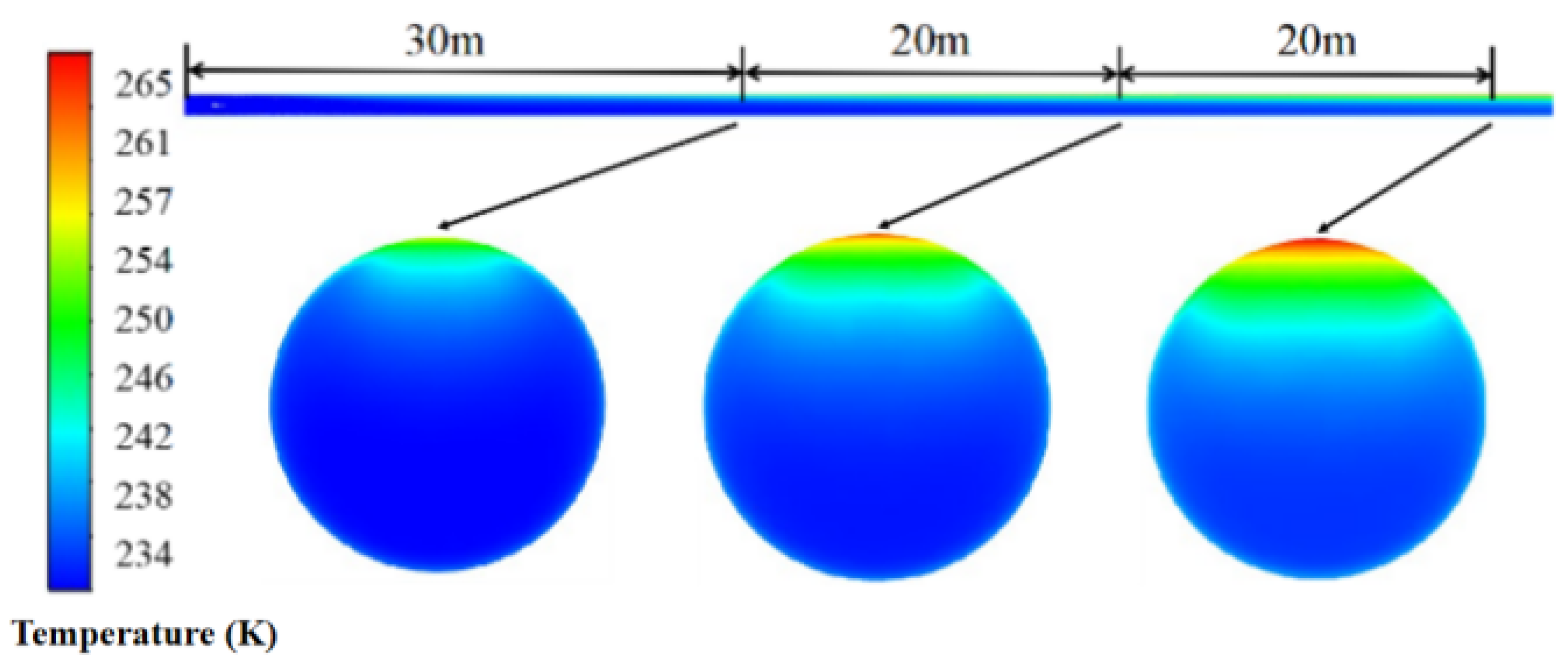
During the pipeline pre-cooling process, nitrogen absorbs heat, thus leading to an increase in temperature and a decrease in density. The near-wall nitrogen experiences a higher temperature rise rate compared to the nitrogen within the pipe. The high-temperature nitrogen near the wall rises along the pipe wall, while the lower-temperature nitrogen sinks. This results in a temperature difference between the top and bottom of the pipeline, as shown in Figure 5.

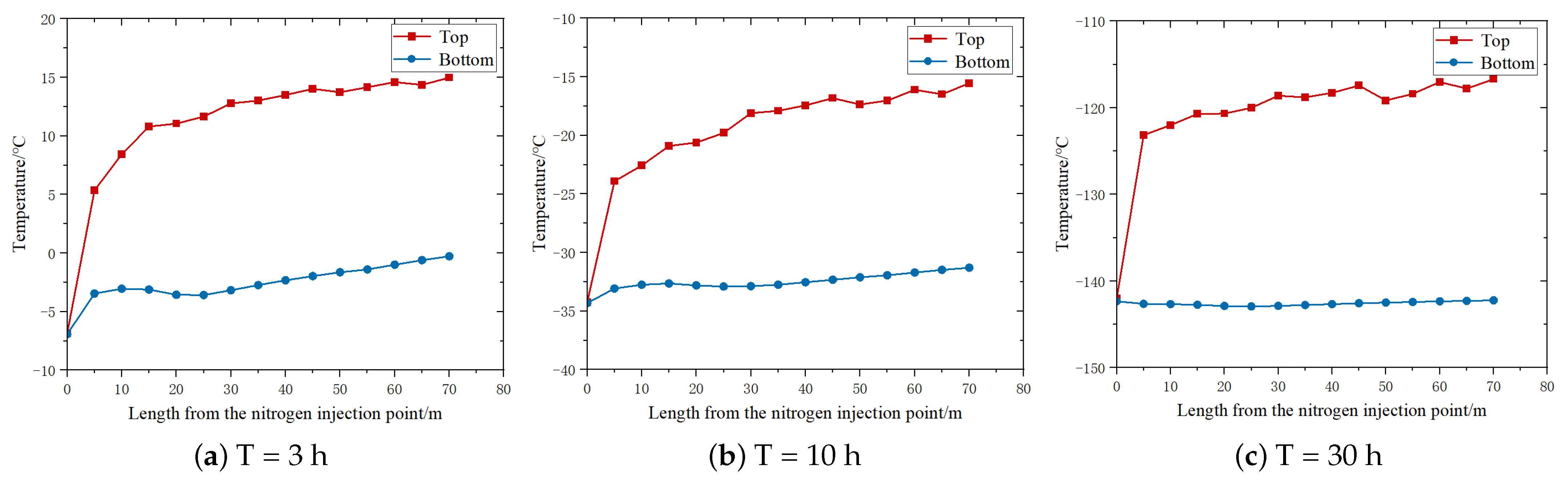
Taking the 46 in pipeline as an example, under the conditions of an ambient temperature of 23 °C and a nitrogen flow velocity of 2.5 m/s, the temperature variation curves at the top and bottom during the pre-cooling process were obtained, as shown in Figure 6.

During the initial stage of pre-cooling (T = 3 h), there was a significant temperature difference between the pipeline and the nitrogen. The nitrogen temperature near the wall rose rapidly and flowed upwards, while the central nitrogen temperature remained relatively low and flowed downward near the wall of inlet. As a result, there was a significant difference in the heat transfer between the top and bottom of the pipeline, thus leading to a rapid increase in the temperature difference. With increasing distance, the nitrogen absorbed heat, thereby raising the overall temperature level and reducing the temperature difference between the nitrogen and the pipeline. Consequently, the difference in heat transfer between the top and bottom of the pipeline decreased, and the top-to-bottom temperature difference tended to level off. During the pre-cooling process, the lower-temperature nitrogen continued to flow toward the bottom of the pipeline. The difference in the heat transfer between the top and bottom of the pipeline accumulated over time and distance from the nitrogen injection point. By the mid-stage of the pre-cooling (T = 10 h), the temperature variation at the bottom of the pipeline had reduced compared to the initial stage, and the temperature variation trend at the top remained relatively stable.

In the late stage of pre-cooling (T = 30 h), there was no temperature recovery phenomenon at the bottom of the pipeline with increasing distance. The bottom temperature remained relatively constant, while the temperature variation trend at the top remained unchanged. In the later stage, the top-to-bottom temperature difference further increased compared to the early and mid-stages of the pre-cooling.

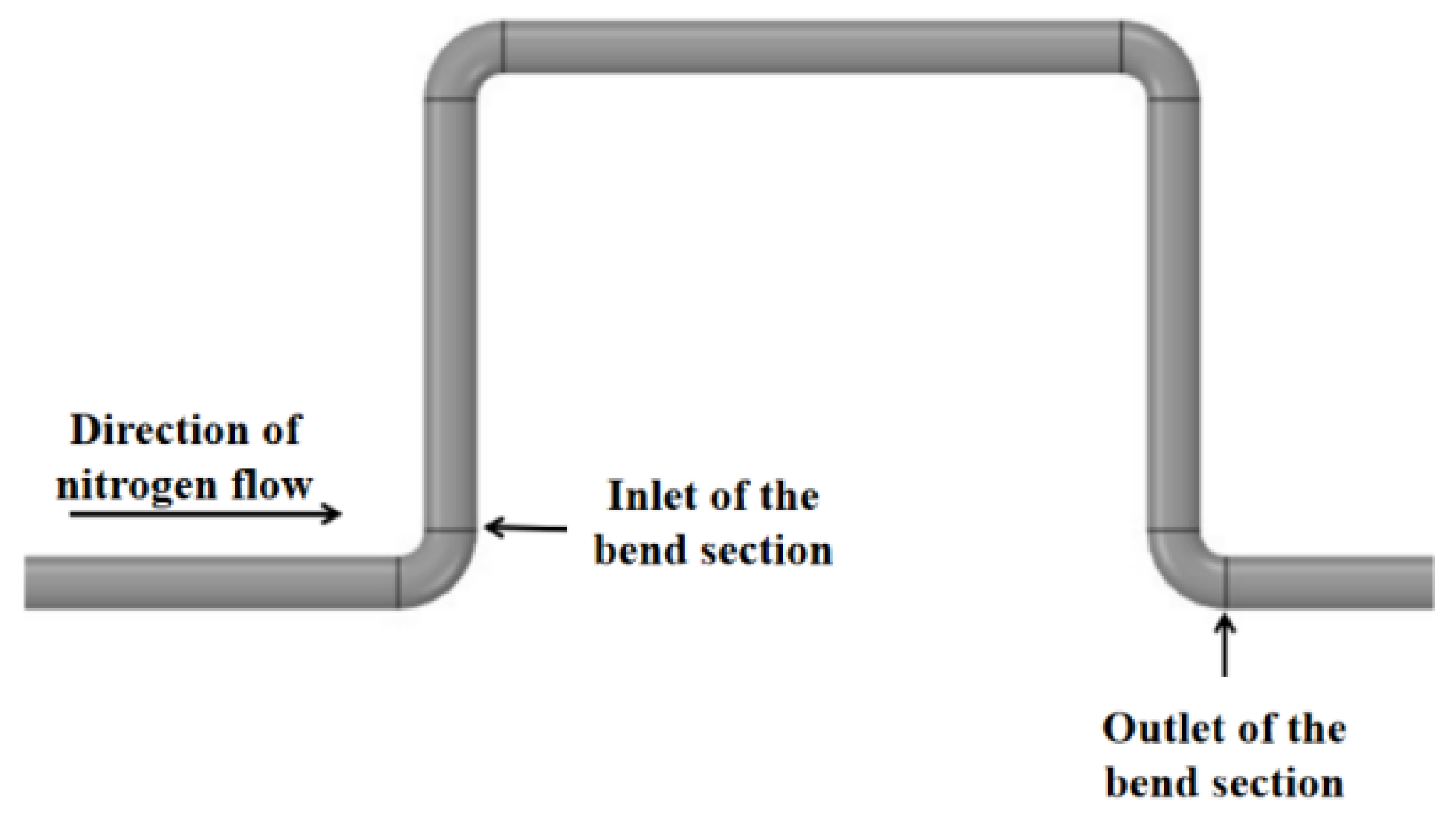
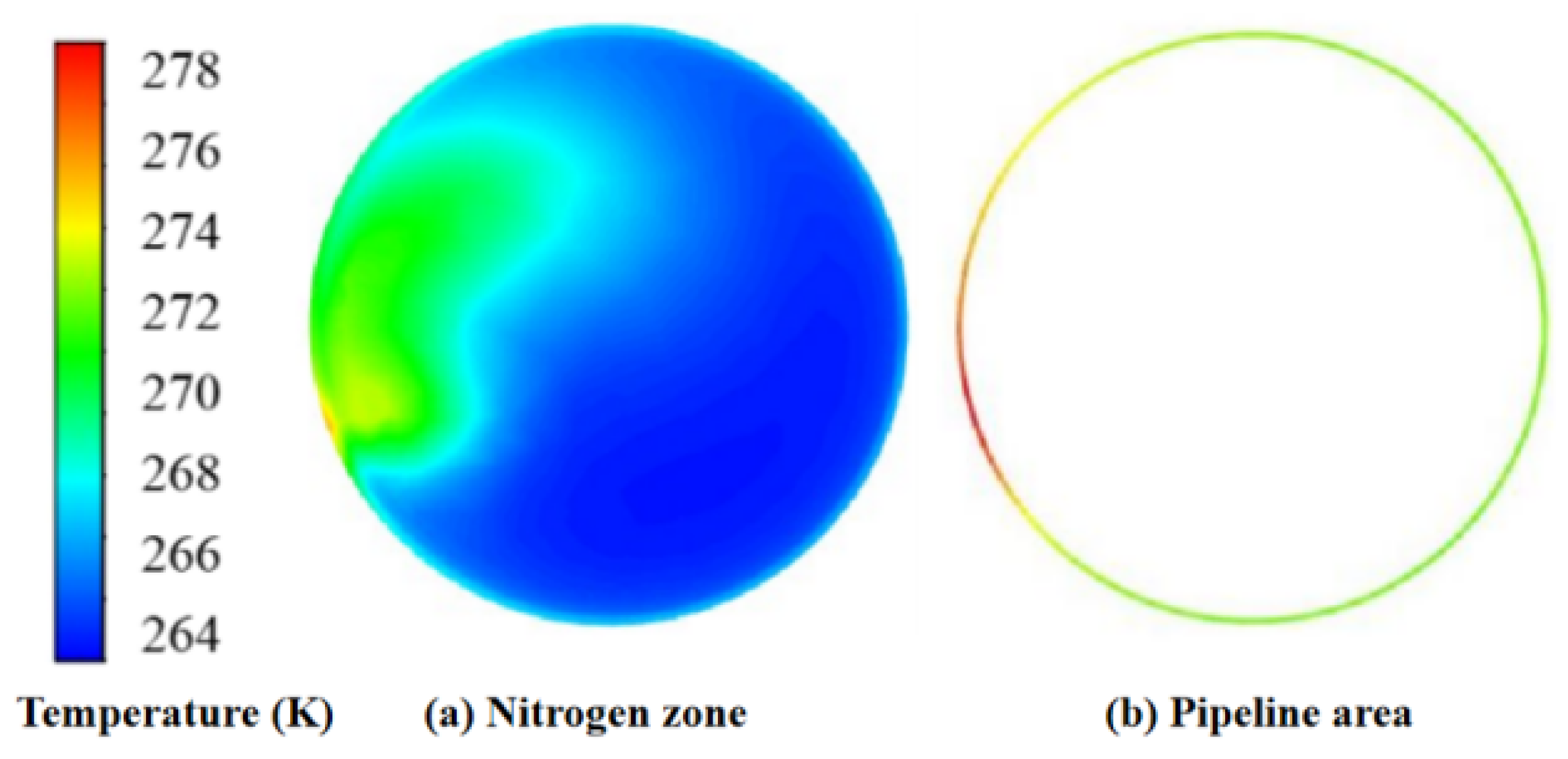
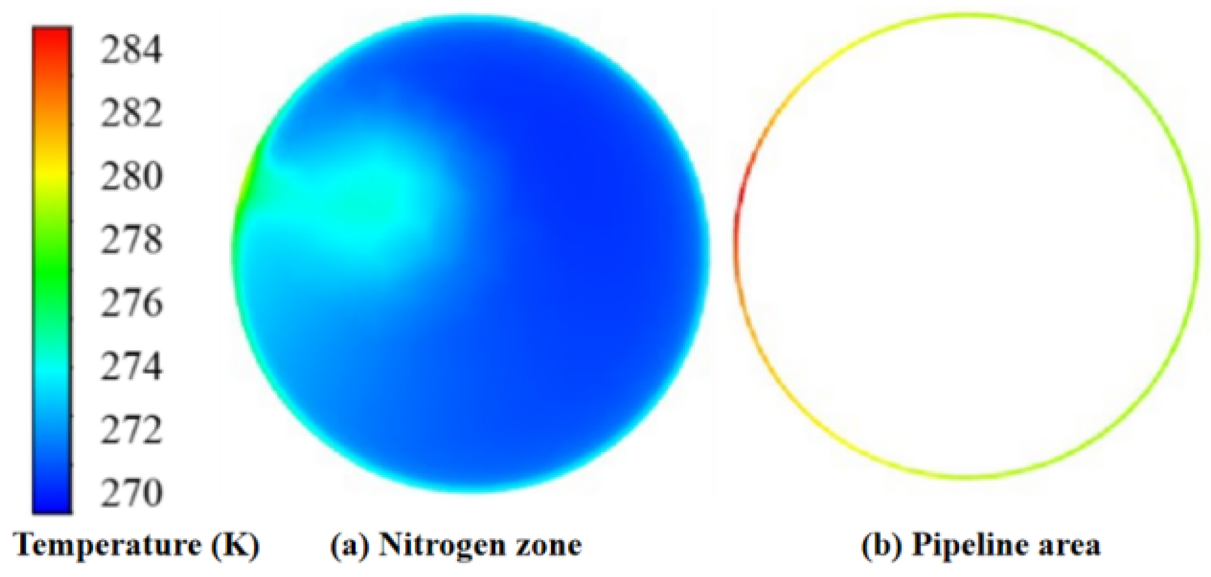
As shown in Figure 7, at the expansion bend corner, the flow of nitrogen was affected by the curvature of the bend, which, in turn, influenced the results of the pipeline pre-cooling. This phenomenon caused a shift in the position of the maximum temperature difference. As shown in Figure 8, due to the centrifugal force, the higher-temperature nitrogen at the top diverted toward the inner side of the bend pipe. Consequently, the position of the highest temperature in the pipeline shifted from the top to the inner wall of the bend pipe.

Due to the impact of the bend section, the turbulence of the nitrogen intensified and the internal mixing became more pronounced. The phenomenon of the nitrogen temperature stratification weakened, thus leading to a reduced temperature difference in the bend section compared to the straight-pipe section. Additionally, at the exit of the bend pipe, the temperature distribution of nitrogen and the pipeline became more uniform, as shown in Figure 9.

4. Discussion

4.1. Influence of Different Nitrogen Injection Velocities

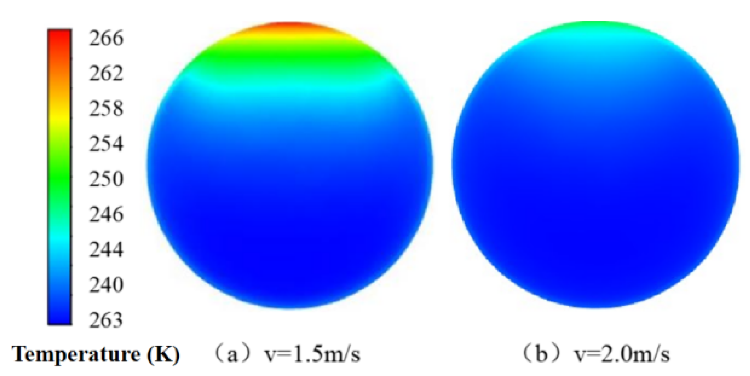
The temperature contour maps of the pipeline wall at different nitrogen injection velocities are shown in Figure 10. With an increase in the nitrogen flow velocity, the turbulent effect of nitrogen intensifies, thereby suppressing nitrogen thermal circulation and alleviating the phenomenon of high- and low-temperature zones. This improvement enhances the effectiveness of pipeline pre-cooling.

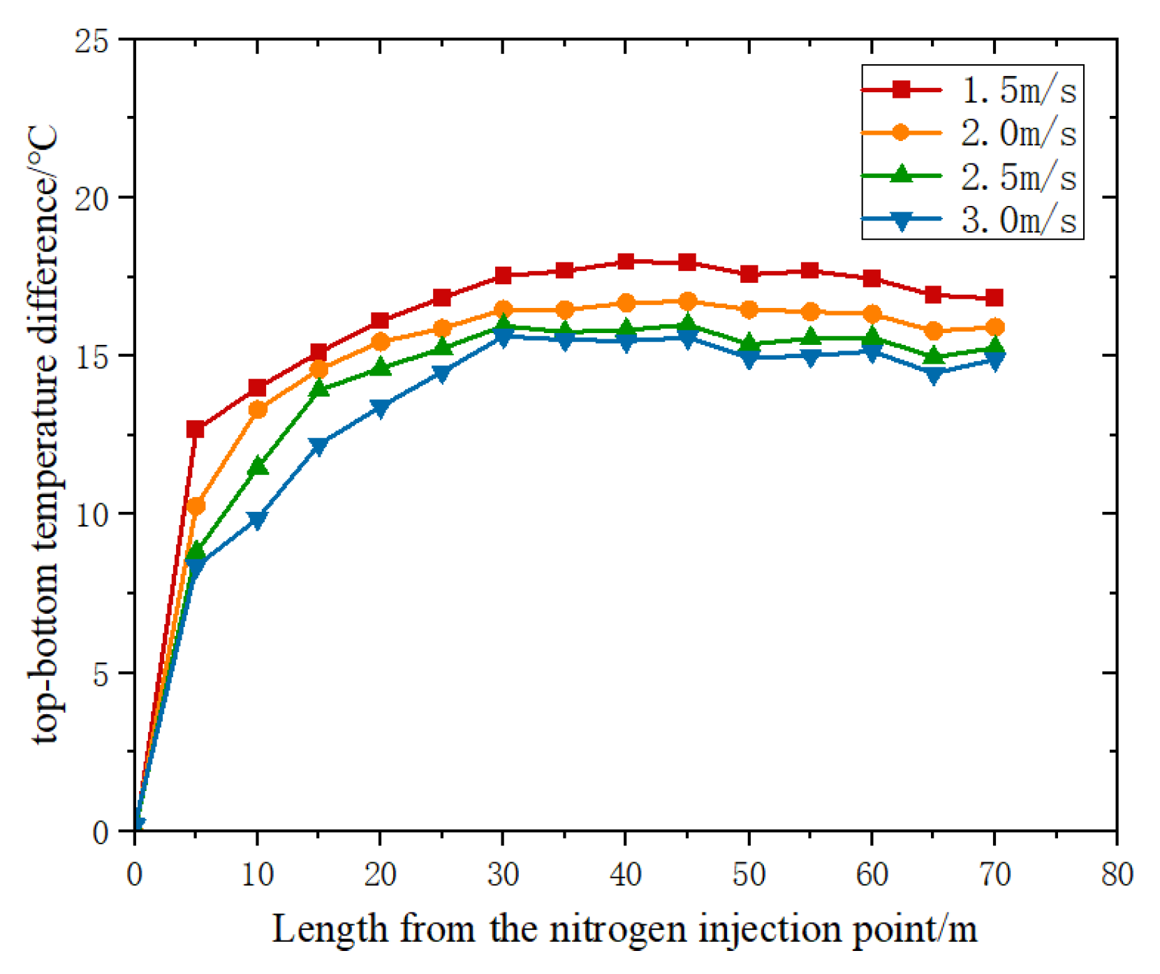
The top-to-bottom temperature difference in the early stage of pre-cooling is shown in Figure 11. At different flow velocities, the top-to-bottom temperature difference rapidly increased near the inlet, whereby it gradually stabilized and peaked before slowly decreasing. Under v = 1.5 m/s, the maximum top-to-bottom temperature difference reached 18 °C. This was attributed to the continuous flow of low-temperature nitrogen toward the bottom of the pipeline near the inlet. This resulted in a faster rate of temperature decrease at the bottom of the pipeline compared to the top, which led to a rapid increase in the temperature difference between the top and bottom. With increasing distance, the overall temperature of the low-temperature nitrogen rose. This resulted in a reduction in both the heat transfer difference between the top and bottom of the pipeline and the rate of increase in the temperature difference between the top and bottom. After a thorough heat exchange in the front half of the pipeline, the overall temperature of the nitrogen rose, and the axial temperature distribution became more uniform. Consequently, the temperature drop rate at the bottom of the pipeline further decreased, and the top-to-bottom temperature difference decreased slowly.

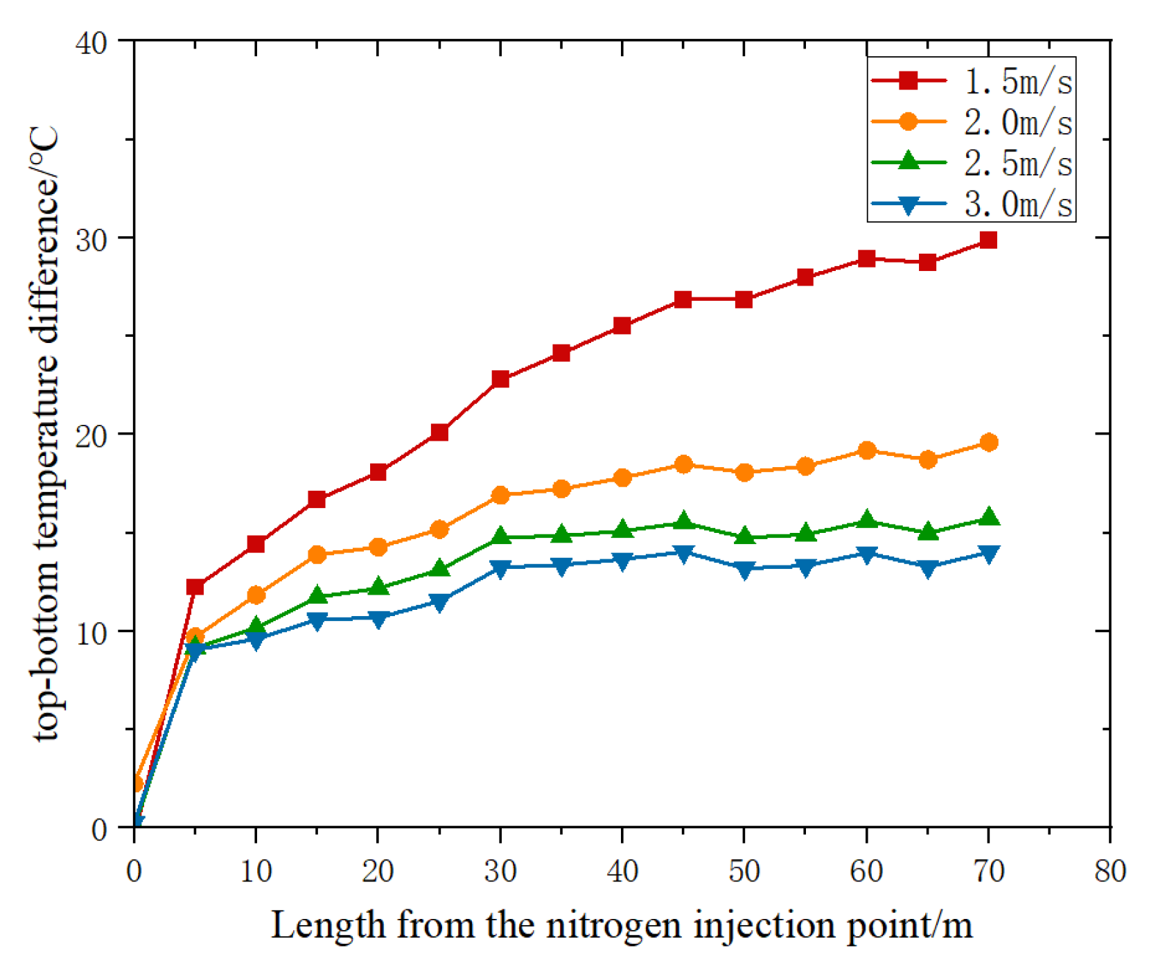
As shown in Figure 12, the top-to-bottom temperature difference gradually increased with distance by the mid-stage of the pre-cooling, and the position of the maximum top-to-bottom temperature difference shifted rearward, ultimately appearing at the end of the pipeline. With an increase in the nitrogen flow velocity, the turbulence intensified, resulting in enhanced convective heat transfer inside the pipeline. This led to a reduction in the top-to-bottom temperature difference. At v = 2 m/s, the reduction in the top-to-bottom temperature difference was the greatest, reaching 50% compared to v = 1.5 m/s. However, at v = 2.5 m/s and 3 m/s, the reduction in the top-to-bottom temperature difference was relatively small. The analysis indicated that, at v = 1.5 m/s, the nitrogen injection rate was too low, and as the length from the injection point increased, the pre-cooling effect at the top of the pipeline significantly weakened. Due to the continuous flow of the cold nitrogen gas toward the bottom of the pipeline, the temperature level at the bottom remained lower, thereby causing the temperature difference between the top and bottom to gradually increase with distance. This ultimately resulted in a significant temperature difference between the top and bottom.

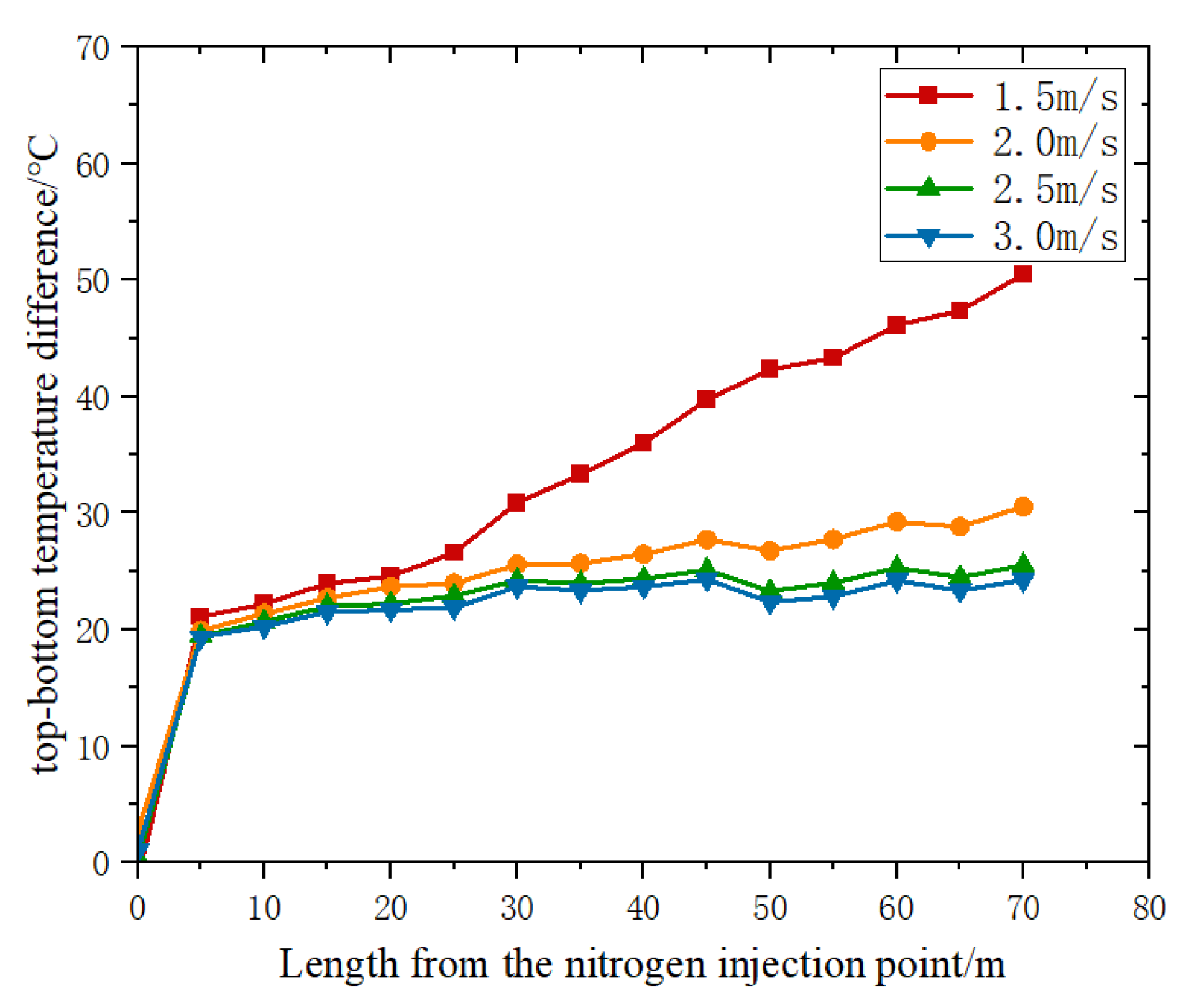
As shown in Figure 13, the difference in the heat transfer effectiveness between the top and bottom of the pipeline accumulated over time. By the late stage of the pre-cooling, the top-to-bottom temperature difference further increased compared to the mid-stage of pre-cooling. Under a nitrogen flow velocity of 1.5 m/s, the top-to-bottom temperature difference gradually increased with distance, and the maximum difference exceeded 50 °C. However, under nitrogen flow velocities of 2.0 m/s, 2.5 m/s, and 3.0 m/s, there was no significant increase in the top-to-bottom temperature difference with distance.

4.2. The Analysis of Factors Influencing the Top-to-Bottom Temperature Difference

During the pipeline pre-cooling process, the flow of nitrogen gas inside the pipeline involved both mixed convection, including natural convection and forced convection. The top-to-bottom temperature difference in the pipeline was primarily caused by natural convection occurring on the cross-section of the pipeline. Here, the Grashof number (Gr) and the Grashof number divided by the square of the Reynolds number (Gr/Re²) were used as discriminant criteria for the analysis.

• Grashof number (Gr):

  $$\mathrm{Gr}=\frac{g{\alpha }_v\mathrm{\Delta }t{L}^3}{{\upsilon }^2}.$$

  (11)
• Gr/Re²:

  $$\frac{\mathrm{Gr}}{{\mathrm{Re}}^2}=\frac{g{\alpha }_v\mathrm{\Delta }tL}{u^2}.$$

  (12)

The Grashof number (Gr) represents the ratio of the buoyancy force to viscous force, and it reflects the intensity of natural convection. On the other hand, Gr/Re² represents the ratio of the buoyancy force to inertial force, thereby indicating the relative magnitude of the effects of natural convection and forced convection. A higher value of Gr and Gr/Re² indicates a stronger influence of natural convection.

Based on a nitrogen gas velocity of 1.5 m/s, the Grashof number (Gr) and Grashof number divided by Reynolds number squared (Gr/Re²) were calculated at different locations for the nitrogen gas temperature and pipe wall temperature, as shown in

Table 1. Gr at different positions of the pipeline at 1.5m/s with nitrogen fluid.

Length from the Nitrogen Injection Point (m)	T = 3 h	T = 10 h
5	$5.93\times {10}^{10}$	$5.39\times {10}^{10}$
10	$5.57\times {10}^{10}$	$5.21\times {10}^{10}$
20	$5.25\times {10}^{10}$	$5.01\times {10}^{10}$
30	$4.95\times {10}^{10}$	$5.17\times {10}^{10}$
40	$4.66\times {10}^{10}$	$5.19\times {10}^{10}$
50	$4.44\times {10}^{10}$	$5.26\times {10}^{10}$
60	$4.19\times {10}^{10}$	$5.19\times {10}^{10}$
70	$4.01\times {10}^{10}$	$5.17\times {10}^{10}$

and

Table 2. Gr/Re² at different positions of the pipeline at 1.5 m/s with nitrogen fluid.

Length from the Nitrogen Injection Point (m)	T = 3 h	T = 10 h
5	2.911	1.825
10	2.744	1.766
20	2.624	1.715
30	2.512	1.789
40	2.390	1.812
50	2.300	1.852
60	2.189	1.840
70	2.108	1.848

. Under the same operating conditions, Gr and Gr/Re² were found to be positively correlated with the top–bottom temperature difference. The variation trends of Gr and Gr/Re² were generally consistent with the changes in the top–bottom temperature difference observed in Figure 11 and Figure 12.

During the early stage of pre-cooling, Gr and Gr/Re² were relatively large at the inlet, indicating significant buoyancy and natural convection effects, which led to a rapid increase in the top–bottom temperature difference. In the later sections of the pipeline, Gr and Gr/Re² gradually decreased, resulting in a gradual reduction in the top–bottom temperature difference. In the mid-stage of the pre-cooling, Gr and Gr/Re² remained relatively large at the inlet, thereby causing a rapid increase in the top–bottom temperature difference. As the length of the pipeline increased, Gr and Gr/Re² continued to grow, further amplifying the top–bottom temperature difference.

The temperature drop rates in the pipeline were noted at different inlet flow rates, as shown in

Table 3. Average temperature drop rate of the pipeline under different flow velocities.

Flow Velocity (m/s)	Top Average Temperature Drop Rate (°C/h)	Bottom Average Temperature Drop Rate (°C/h)
1.5	4.32	5.40
2.0	4.57	5.39
2.5	4.65	5.40
3.0	4.69	5.41

. As the nitrogen flow rate increased, the nitrogen injection amount increased and the temperature drop rate at the top of the pipeline significantly increased. This was because, during the pre-cooling process, low-temperature nitrogen continuously flowed toward the bottom of the pipeline, thereby ensuring effective cooling at the bottom. With increasing nitrogen flow rate, there was no significant increase in the temperature drop rate at the bottom. At the same time, the increase in the temperature drop rate at the top was limited with increasing nitrogen injection amounts. To balance the nitrogen consumption and pipeline temperature drop rate, a nitrogen flow rate of 2.5 m/s provided the optimal overall pre-cooling effect.

4.3. Influence of Different Pipe Diameters

4.3.1. Large-Diameter Pipes

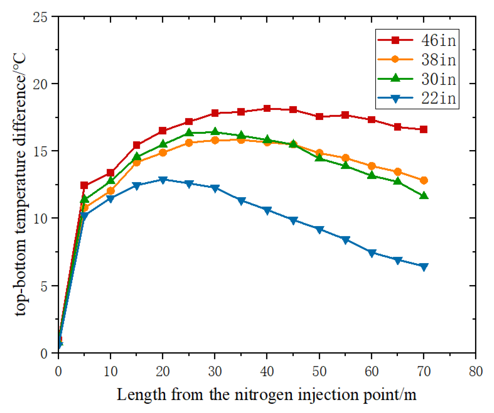
The temperature difference between the top and bottom of the large-diameter pipes (46 in, 38 in, 30 in, and 22 in) during the initial stage of the pre-cooling were noted, as shown in Figure 14. After 3 h of pre-cooling, the temperature difference distribution along the length of the pipes was found to be consistent for the different diameters. It rapidly increased near the inlet and then gradually decreased. Additionally, as the diameter decreased, the temperature difference initially increased and then decreased, with the location of the maximum temperature difference gradually moving closer to the inlet.

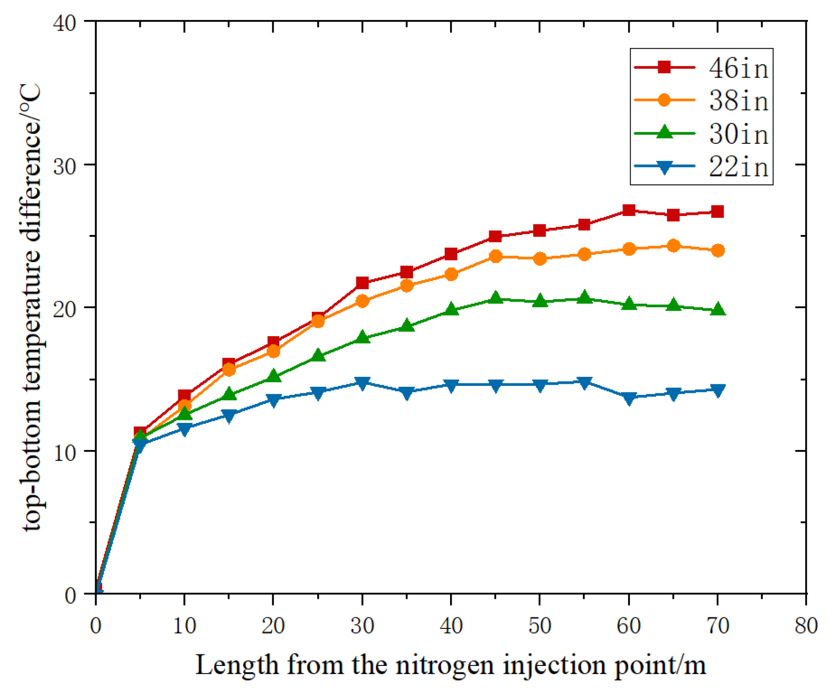
As the pre-cooling process progressed, the position of the maximum top-to-bottom temperature difference gradually shifted downstream. Throughout the entire length of the pipe, the top-to-bottom temperature difference gradually increased and reached its maximum value at the end of the pipe. When d = 46 in, it reached a maximum of 27 °C, as shown in Figure 15. Smaller diameters resulted in enhanced turbulent effects, which improved heat transfer and reduced the top-to-bottom temperature difference. However, it is important to note that as the diameter decreases, the reduction in the top-to-bottom temperature difference becomes more significant.

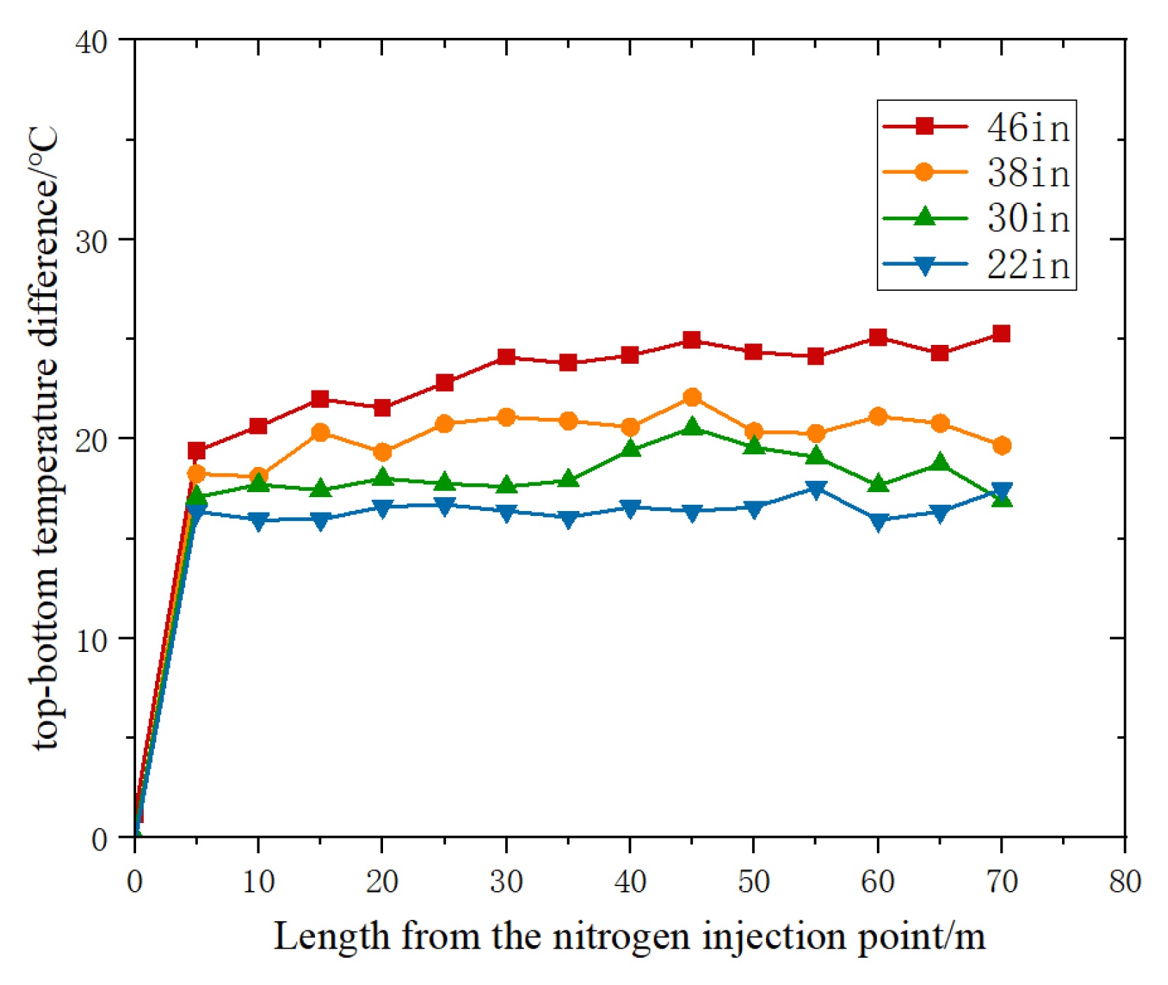
As shown in Figure 16, in the later stages of pre-cooling, the top-to-bottom temperature difference remained relatively constant with some fluctuations. At the same time, as the diameter decreased, the enhanced turbulent effects improved heat transfer and reduced the top-to-bottom temperature difference, although the reduction was less significant. The average top-to-bottom temperature difference gradually decreased from 23 °C to 16 °C.

Based on the nitrogen gas temperatures and pipe wall temperatures at different positions within the pipe with a diameter of 46 in, the Gr and Gr/Re² at different positions were calculated, as shown in

Table 4. Gr at different positions of pipes with a diameter of 46 in.

Length from the Nitrogen Injection Point (m)	T = 3 h	T = 10 h
5	$6.12\times {10}^{10}$	$5.03\times {10}^{10}$
10	$5.75\times {10}^{10}$	$4.95\times {10}^{10}$
20	$5.46\times {10}^{10}$	$4.68\times {10}^{10}$
30	$5.09\times {10}^{10}$	$4.84\times {10}^{10}$
40	$4.77\times {10}^{10}$	$4.89\times {10}^{10}$
50	$4.54\times {10}^{10}$	$4.95\times {10}^{10}$
60	$4.29\times {10}^{10}$	$4.90\times {10}^{10}$
70	$4.09\times {10}^{10}$	$4.91\times {10}^{10}$

and

Table 5. Gr/Re² at different positions of pipes with a diameter of 46 in.

Length from the Nitrogen Injection Point (m)	T = 3 h	T = 10 h
5	3.302	1.399
10	3.117	1.378
20	3.005	1.314
30	2.845	1.371
40	2.697	1.396
50	2.595	1.423
60	2.470	1.418
70	2.377	1.430

. The trends of Gr and Gr/Re² with respect to the top-to-bottom temperature difference were consistent with those shown in Table 1 and Table 2. In the early stage of pre-cooling, the Gr and Gr/Re² were relatively large at the inlet, resulting in a rapid increase in the top-to-bottom temperature difference. Toward the later sections of the pipe, the Gr and Gr/Re² decreased slowly, and the top-to-bottom temperature difference decreased gradually. In the middle stage of pre-cooling, the Gr and Gr/Re² remained relatively large at the inlet, thereby leading to a rapid increase in the top-to-bottom temperature difference. In the later sections of the pipe, both the top-to-bottom temperature difference and Gr/Re² increased slowly.

The different temperature reduction rates for various pipe diameters are shown in

Table 6. Average temperature drop rate of a large-diameter pipe under different pipe diameters.

Pipe Diameter (in)	Top Average Temperature Drop Rate (°C/h)	Bottom Average Temperature Drop Rate (°C/h)
46	3.62	5.21
38	3.73	5.11
30	3.86	5.00
22	4.00	4.82

. As the diameter of the pipe decreased, the heat exchange between the gas and the wall intensified, resulting in an increase in the average temperature reduction rate at the top and a decrease at the bottom. However, due to the reduction in pipe diameter, the nitrogen gas flow rate decreased, offsetting the enhanced heat exchange due to turbulence. As a result, the overall temperature reduction rate remained approximately the same at around 4.4 °C/h.

4.3.2. Small-Diameter Pipes

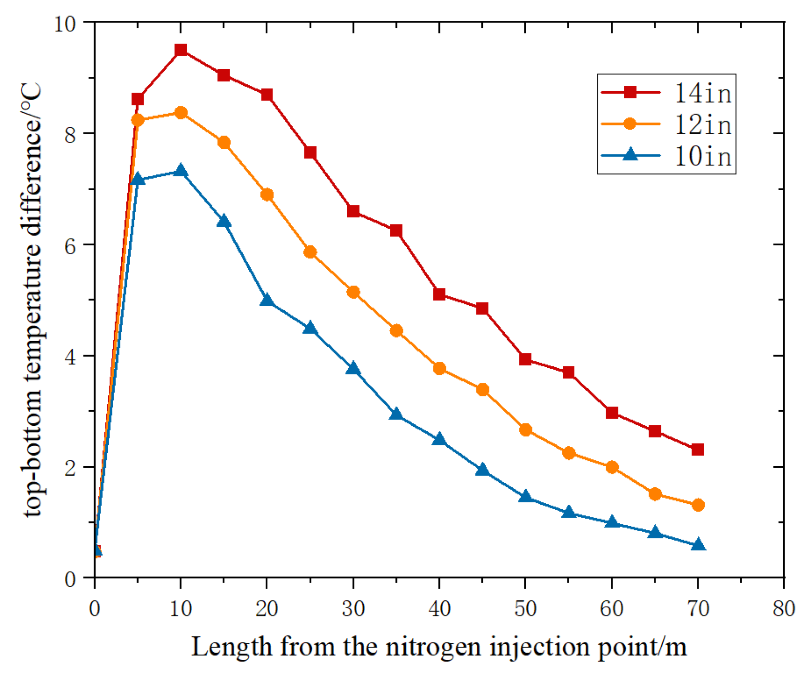
In the case of small-diameter pipes (14 in, 12 in, and 10 in), the effect of the pipe diameter on the temperature difference between the top and bottom of the pipes followed a pattern similar to that of the large-diameter pipes. As shown in Figure 17, the temperature difference increased rapidly near the inlet and then gradually decreased after reaching a maximum value at a certain position along the pipe. Additionally, smaller pipe diameters result in smaller temperature differences between the top and bottom of the pipe, and the location of the maximum temperature difference shifted closer to the pipe inlet.

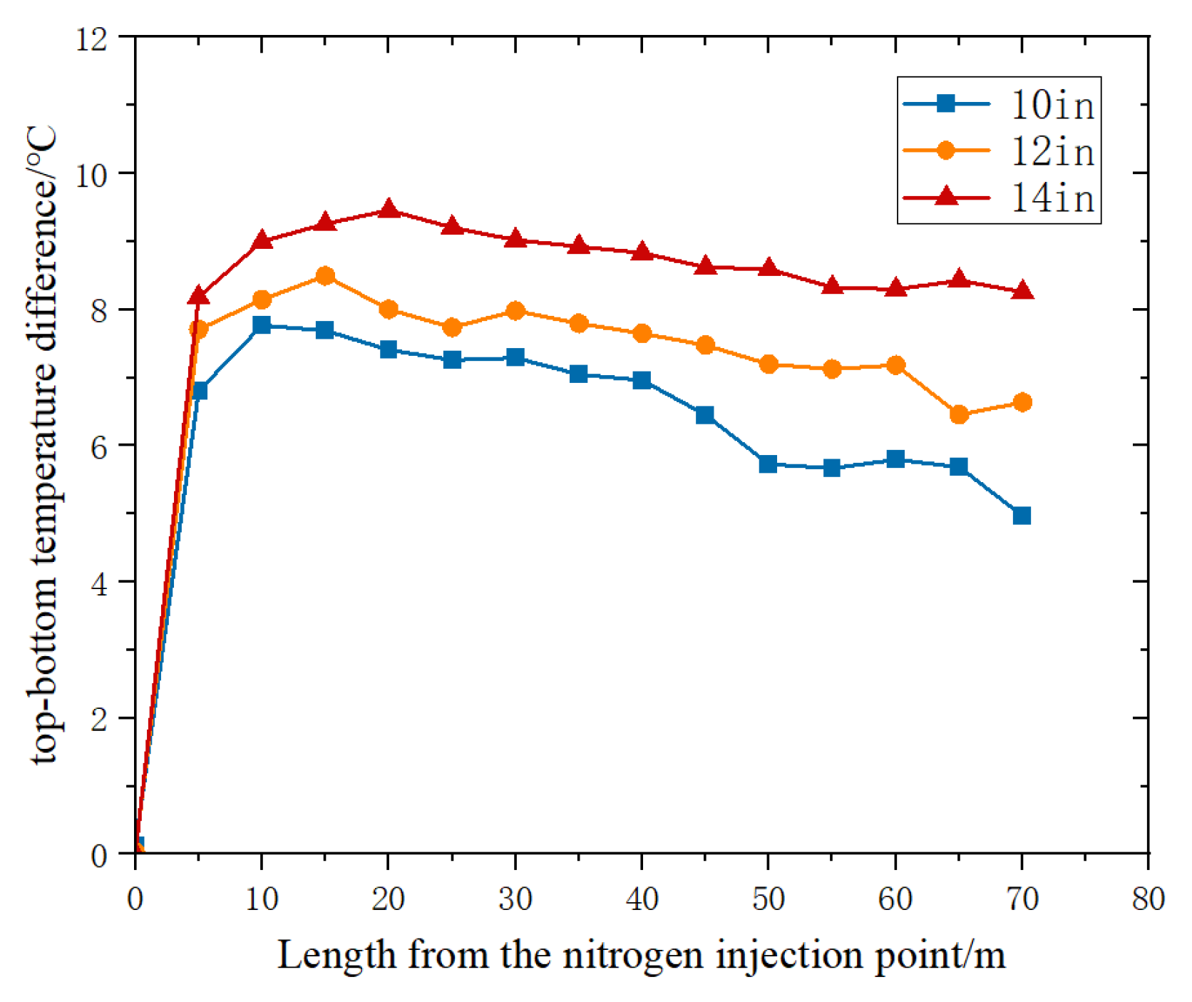
As shown in Figure 18, unlike the case with large-diameter pipelines, during the pre-cooling process of small-diameter pipelines, the temperature difference between the top and bottom remained constant from the front to the back end of the pipeline. The temperature difference between the top and bottom of the pipe remained constant along the length of the pipe. This can be attributed to the fact that, with smaller pipe diameters, the nitrogen gas inside the pipe settles and stabilizes near the front end of the pipe, thus leading to a constant temperature difference between the top and bottom of the pipe.

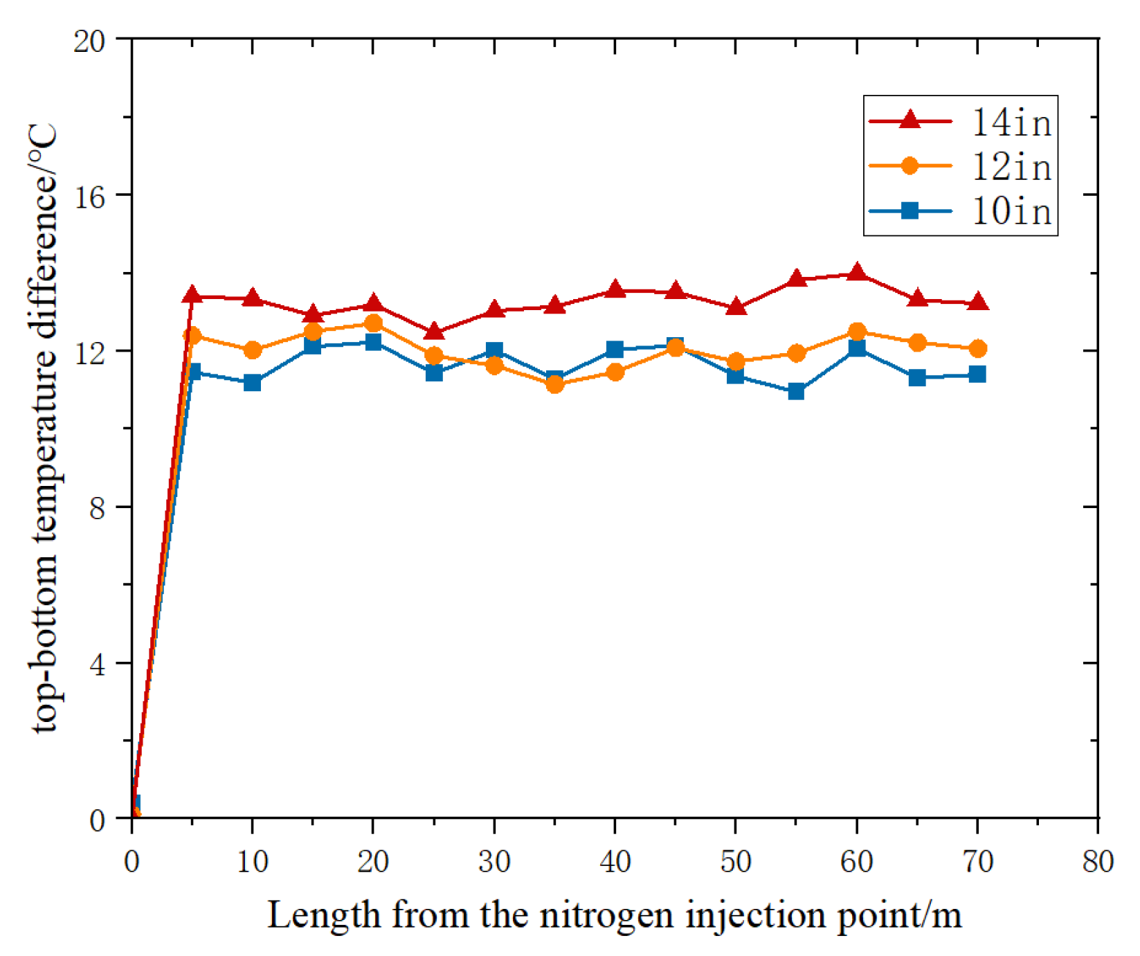
As shown in Figure 19, during the later stages of pre-cooling, the temperature difference between the top and bottom remained essentially unchanged with increasing distance. Additionally, the fluctuation range of the temperature difference in small-diameter pipelines was smaller. As the pipe diameter decreased, the extent of the reduction in the temperature difference between the top and bottom was also smaller.

As shown in

Table 7. The Gr at different positions of pipes with a diameter of 14 in.

Length from the Nitrogen Injection Point (m)	T = 3 h	T = 10 h
5	$1.67\times {10}^9$	$1.55\times {10}^9$
10	$1.50\times {10}^9$	$1.42\times {10}^9$
20	$1.22\times {10}^9$	$1.34\times {10}^9$
30	$1.01\times {10}^9$	$1.28\times {10}^9$
40	$8.36\times {10}^8$	$1.22\times {10}^9$
50	$6.89\times {10}^8$	$1.18\times {10}^9$
60	$5.66\times {10}^8$	$1.12\times {10}^9$
70	$4.65\times {10}^8$	$1.07\times {10}^9$

and

Table 8. The Gr/Re² at different positions of pipes with a diameter of 14 in.

Length from the Nitrogen Injection Point (m)	T = 3 h	T = 10 h
5	0.958	0.454
10	0.877	0.422
20	0.736	0.407
30	0.625	0.395
40	0.527	0.386
50	0.442	0.377
60	0.368	0.366
70	0.306	0.357

, based on the nitrogen gas temperature and pipe wall temperature at different positions of a pipe with a diameter of 14 in, the Gr and the Gr/Re² discriminants at different positions were calculated. When the diameter was reduced to 14 in, both the Gr and Gr/Re² were smaller compared to when it was 46 in. According to the Gr/Re² discriminant, when 0.1 < Gr/Re² < 10, it indicates mixed convection. As shown in Figure 13 and Table 5, the Gr/Re² in the latter part of the 14 in diameter pipe was smaller, thus indicating weaker natural convection. The top-to-bottom temperature difference was less than 10 °C, which is within the acceptable error range; therefore, the effect of the natural convection can be largely ignored. Consequently, the heat transfer process inside the pipe could be approximated as a forced-convection, heat transfer process.

As shown in

Table 9. Average temperature drop rate of a small-diameter pipe under different pipe diameters.

Pipe Diameter (in)	Top Average Temperature Drop Rate (°C/h)	Bottom Average Temperature Drop Rate (°C/h)
14	4.94	5.38
12	4.96	5.36
10	4.92	5.31

, in the late stage of the pre-cooling process in the small-diameter pipes, the temperature difference between the top and bottom remained relatively constant with increasing distance along the pipe. Furthermore, compared to the large-diameter pipes, the small-diameter pipes exhibited smaller fluctuations in temperature difference. The reduction in the temperature difference was also less pronounced as the pipe diameter decreased.

5. Conclusions

This paper conducted a numerical simulation analysis on the low-temperature, nitrogen pre-cooling process of LNG unloading pipelines. These numerical simulations were performed using Fluent software for different nitrogen injection rates and pipe diameters. The following conclusions were obtained:

• In large-diameter unloading pipelines, the pre-cooling heat transfer is a combination of forced convection and natural convection, and the effect of natural convection should not be neglected. Due to the natural convection inside the pipe, there is a stratification of nitrogen gas with different temperatures, thereby resulting in temperature differences between the top and bottom of the pipeline, with higher temperature drop rates at the bottom compared to the top. As the pipe diameter decreases, the temperature difference between the top and bottom of the pipeline also decreases. For small-diameter pipelines (14 inches and below), the influence of natural convection can be essentially disregarded.
• Within a certain range, increasing the nitrogen injection velocity can improve the pipeline pre-cooling rate and reduce the temperature difference between the top and bottom of the pipeline. However, it also leads to increased nitrogen consumption. For pipelines with a diameter of 46 in, using a nitrogen injection velocity of 2.5 m/s can reduce nitrogen consumption while ensuring the pre-cooling rate. For other pipe diameters, further research is needed to determine the optimal diameter.
• Under certain nitrogen injection velocity conditions, smaller pipe diameters result in smaller temperature differences between the top and bottom of the pipeline. For large-diameter pipes (22 in and above), the average temperature drop rate remains relatively constant. In contrast, for small-diameter pipes (14 in and below), the average temperature drop rate gradually decreases as the pipe diameter decreases.
• Gr and Gr/Re² reflect the relative strengths of natural convection and forced convection. The variation pattern of temperature difference between the top and bottom of the pipe cross-section is consistent with Gr and Gr/Re². Gr and Gr/Re² can be used to discern the variation pattern of the temperature difference between the top and bottom of different cross-sections of the pipe.

References

- Wang, Z.Y.; Luo, D.K.; Wang, G. Developing rules and prospect of natural gas utilization in China. Nat. Gas Ind. 2014, 34, 121–127. [Google Scholar]
- Gao, W.X. Safety and development prospect of liquefied natural gas (LNG) storage and transportation. Petrochem. Ind. Technol. 2018, 25, 68–69. [Google Scholar]
- Song, Y.G. Pre-cooling Analysis of Typical Pipeline in LNG Terminal Based on ANSYS. Gas Heat 2022, 42, 18–23. [Google Scholar]
- Chen, F.; Zhang, C.; Chen, R.Y.; Liu, Y.H.; Wang, Y.Q.; Wang, X.H. A temperature-stress model for pipeline pre-cooling in an LNG receiving terminal. Nat. Gas Ind. 2019, 39, 102–106. [Google Scholar]
- Burke, J.C.; Byrnes, W.R.; Post, A.H.; Ruccia, F.E. Pressurized cooldown of cryogenic transfer lines. Adv. Cryog. Eng. 1960, 4, 378–394. [Google Scholar]
- Hedayatpour, A.; Antar, B.; Kawaji, M. Analytical and numerical investigation of cryogenic transfer line chilldown. In Proceedings of the 26th Joint Propulsion Conference, Orlando, FL, USA, 16–18 July 1990. [Google Scholar]
- Bendik, N.T.; Smirnov, S.K.; Blinkov, Y.L. Calculation of stationary heat transfer zone in conduits under cooldown. Cryogenics 1979, 19, 477–482. [Google Scholar] [CrossRef]
- Yuan, K.; Ji, Y.; Chung, J.N.; Shyy, W. Cryogenic boiling and two-phase flow during pipe chilldown in earth and reduced gravity. J. Low Temp. Phys. 2008, 150, 101–122. [Google Scholar] [CrossRef]
- Liao, J.; Mei, R.; Klausner, J. A film boiling model for cryogenic chilldown at low mass flux inside a horizontal pipeline. Heat Mass Transf. 2006, 42, 891–900. [Google Scholar] [CrossRef]
- Schepper, S.; Heynderickx, G.J.; Marin, G.B. Modeling the evaporation of a hydrocarbon feedstock in the convection section of a steam cracker. Int. Comput. Chem. Eng. 2009, 33, 122–132. [Google Scholar] [CrossRef]
- Melideo, D.; Baraldi, D.; Galassi, M.C.; Cebolla, R.O.; Iborra, B.A.; Moretto, P. CFD model performance benchmark of fast filling simulations of hydrogen tanks with pre-cooling. Int. J. Hydrogen Energy 2014, 39, 4389–4395. [Google Scholar] [CrossRef]
- Lu, J.; Xu, S.; Deng, J.; Wu, W.; Wu, H.; Yang, Z. Numerical prediction of emperature field for cargo containment system (CCS) of LNG carriers during pre-cooling operations. Int. J. Nat. Gas Sci. Eng. 2016, 29, 382–391. [Google Scholar] [CrossRef]
- Hu, H.; Chung, J.N.; Amber, S.H. An experimental study on flow patterns and heat transfer characteristics during cryogenic chilldown in a vertical pipe. Int. Cryog. 2012, 52, 268–277. [Google Scholar] [CrossRef]
- Velat, C.; Jackson, J.; Klausner, J.F.; Mei, R. Cryogenic two-phase flow during chilldown. Heat Transf. Summer Conf. 2004, 4694, 717–722. [Google Scholar]
- Jin, L.; Seo, M.; Cho, H.; Park, C.; Lee, C.; Jeong, S. Experimental Investigation on Cryogenic Line Chill-Down Process by Using Liquid Nitrogen. In Proceedings of the ASME Summer Heat Transfer Conference, Washington, DC, USA, 10–14 July 2016. [Google Scholar]
- Hartwig, J.; Hu, H.; Styborski, J.; Chung, J.N. Comparison of cryogenic flow boiling in liquid nitrogen and liquid hydrogen chilldown experiments. Int. J. Heat Mass Transf. 2015, 88, 662–673. [Google Scholar] [CrossRef]
- Hartwig, J.; Styborski, J.; McQuillen, J.; Rame, E.; Chung, J.N. Liquid hydrogen line chilldown experiments at high Reynolds Numbers. Optimal chilldown methods. Int. J. Heat Mass Transf. 2019, 137, 703–713. [Google Scholar] [CrossRef]
- Johnson, J.; Hine, S.R. Transient cryogenic chill down process in horizontal and inclined pipes. Int. Cryog. 2015, 71, 7–17. [Google Scholar] [CrossRef]
- Wang, L.; Shi, S.G.; Qu, M.; Wang, J.; Li, Y.; Lei, G. Experimental study on cryogenic chilldown performance through a thick-wall tube. Int. Cryog. 2022, 122, 103436. [Google Scholar] [CrossRef]
- Kashani, A.; Luchinskiy, D.G.; Ponizovskaya-Devine, E.; Khasin, M.; Timucin, D.; Sass, J.; Perotti, J.; Brown, B. Optimization of cryogenic chill down and loading operation using SINDA/FLUINT. Int. Iop Conf. Ser. Mater. Sci. Eng. 2015, 101, 012115. [Google Scholar] [CrossRef]
- Shi, Y.W.; Wang, W.; Kuang, Y.W.; Lin, E.C.; Wang, T.; Zhuan, R.; Zhang, L. Simulation of cryogenic pipeline chill-down with liquid nitrogen. Int. Cryog. Supercond. 2021, 49, 79–87. [Google Scholar]
- Shi, Y.W.; Wang, W.; Zhuan, R.; Zhang, L.; Jin, X. An experimental study on pipeline pre-cooling with cryogenic liquid nitrogen. Int. Cryog. 2021, 6, 45–50. [Google Scholar]
- Yan, J.W.; Li, Z.C.; Zhao, D. Numerical simulation of LNG cryogenic pipe precooling process. Int. Cryog. Supercond. 2014, 42, 10–14. [Google Scholar]
- Cao, X.W.; Ji, J.Y.; Yang, W. Temperature distribution of LNG unloading pipelines during nitrogen pre-cooling. Int. Oil Gas Storage Transp. 2016, 35, 492–497. [Google Scholar]
- Dresar, J.N.V.; Siegwarth, J.D. Cryogenic transfer line chilldown. Int. Adv. Cryog. Eng. 2004, 493, 8–15. [Google Scholar]
- Mohammed, J.; Rasheed, R.; Junaid, F.P.; Roy, K.R. Experimental investigation on the effect of geometry on cryogenic transfer line chilldown. In Proceedings of the 2nd Biennial International Conference on Aerospace and Mechanical Engineering (ICAME), Kollam, India, 17–19 December 2019. [Google Scholar]
- Jo, J.C.; Kang, D.G. CFD Analysis of Thermally Stratified Flow and Conjugate Heat Transfer in a PWR Pressurizer Surgeline. Int. J. Press. Vessel. Technol.-Trans. Asme 2010, 132, 021301. [Google Scholar] [CrossRef]
- Kato, Y.; Fujimoto, K.; Guo, G.; Kawaguchi, M.; Kamigaki, M.; Koutoku, M.; Hongou, H.; Yanagida, H.; Ogata, Y. Heat Transfer Characteristics of Turbulent Flow in Double-90°-Bend Pipes. Int. Energies 2013, 16, 7314. [Google Scholar] [CrossRef]
- Cai, M.Y. Pre-cooling Simulation of Large-diameter Cooling Pipeline. Int. Pipeline Tech. Equip. 2021, 6, 5–8+26. [Google Scholar]
- Hu, H.; Wijeratne, T.K.; Chung, J.N. Two-Phase Flow and Heat Transfer During Chilldown of a Simulated Flexible Metal Hose Using Liquid Nitrogen. Int. J. Low Temp. Phys. 2014, 174, 247–268. [Google Scholar] [CrossRef]
- NIST Chemistry WebBook, SRD 69. Available online: https://webbook.nist.gov/chemistry/ (accessed on 17 March 2023).
Figure 1.
Main dimensions of pipe model.
Figure 2.
Pipeline solid-domain and fluid-domain meshing.
Figure 3.
Temperature variation at the end of pipeline model with different grid numbers.
Figure 4.
A comparison of the calculated results and the field data. (a) Location of the monitoring points. (b) The field data and numerical simulation results.
Figure 5.
The pipe profile temperature.
Figure 6.
The temperature distribution curve of pipe’s top and bottom.
Figure 7.
Position diagram of the bend.
Figure 8.
Temperature distribution at the cross-section of the bend pipe inlet.
Figure 9.
Temperature distribution at the exit of the bend.
Figure 10.
Temperature distribution of the pipeline section under different nitrogen flow rates (for the 70 m position).
Figure 11.
Temperature difference curve at the top and bottom of the pipeline after a 3 h pre-cooling time at different nitrogen flow rates.
Figure 12.
Temperature difference curve at the top and bottom of the pipeline after a 10 h pre-cooling time at different nitrogen flow rates.
Figure 13.
Temperature difference curves at the top and bottom of the pipeline after a 30 h pre-cooling time at different nitrogen flow rates.
Figure 14.
The top and bottom temperature of the large-diameter pipeline with a pre-cooling time of 3 h under different pipe diameters.
Figure 15.
The top and bottom temperature of the large-diameter pipeline with a pre-cooling time of 10 h under different pipe diameters.
Figure 16.
The top and bottom temperature of the large-diameter pipeline with a pre-cooling time of 30 h under different pipe diameters.
Figure 17.
The top and bottom temperature of a small-diameter pipeline with a pre-cooling time of 3 h under different pipe diameters.
Figure 18.
The top and bottom temperature of a small-diameter pipeline with a pre-cooling time of 10 h under different pipe diameters.
Figure 19.
The top and bottom temperatures of a small-diameter pipeline with a pre-cooling time of 30 h under different pipe diameters.