Article

Optimized Dual-Layer Distributed Energy Storage Configuration for Voltage Over-Limit Zoning Governance in Distribution Networks

1
State Grid Fujian Electric Power Co., Ltd., Fuzhou 350007, China
2
State Grid Fujian Electric Power Co., Ltd. Electric Power Science Research Institute, Fuzhou 350007, China
3
Hubei Key Laboratory of Power Equipment & System Security for Integrated Energy, Wuhan 430072, China
4
School of Electrical Engineering and Automation, Wuhan University, Wuhan 430072, China
*
Author to whom correspondence should be addressed.
Energies 2024, 17(8), 1847; https://doi.org/10.3390/en17081847
Submission received: 12 March 2024 / Revised: 3 April 2024 / Accepted: 10 April 2024 / Published: 12 April 2024

Abstract

:
In this study, an optimized dual-layer configuration model is proposed to address voltages that exceed their limits following substantial integration of photovoltaic systems into distribution networks. Initially, the model involved segmenting the distribution network’s voltage zones based on distributed photovoltaic governance resources, thereby elucidating the characteristics and governance requisites for voltages across distinct regions. Subsequently, a governance model for voltage limit exceedances, grounded in optimizing energy storage configurations, was formulated to mitigate photovoltaic power fluctuations by deploying energy storage systems. This model coordinates the reactive power output of photovoltaic installations with the active power consumption of energy storage systems, thereby augmenting voltage autonomy in the power grid. This study leveraged Karush–Kuhn–Tucker (KKT) conditions and the Big-M method to transform the dual-layer model into a single-layer linear model, thereby enhancing solution efficiency and precision. Finally, a simulation was carried out to demonstrate that the strategy proposed from this research not only achieves commendable economic efficiency, but also significantly improves the regional voltage effect by 28.7% compared to the optical storage capacity optimization model.

1. Introduction

As the penetration of distributed generators (DGs) continues to expand, the discrepancy between their variable output and the inadequate alignment with distribution network loads in both spatial and temporal dimensions has become increasingly salient. Restricting the output of such generators would lead to the wastage of renewable resources [1,2,3]. While optimizing the placement and capacity of DG access offers some mitigation, its efficacy remains limited; achieving on-site consumption of renewable energy proves challenging [4]. Early domestic distribution network planning often overlooked the integration of large-scale distributed power sources, particularly within rural grids characterized by limited robustness. The high penetration rates of photovoltaic systems in such contexts exacerbate operational safety concerns, notably the phenomenon of power reverse flow [5]. This transition from a passive to a complex multi-source distribution network heightens the risk of voltages exceeding their limits [6], thereby impinging upon both the utilization of renewable energy within the network, as well as the safe and stable operation of its infrastructure. Consequently, there exists a pressing need for research aimed at optimizing management strategies to address node voltage limit violations that have resulted from the high penetration of photovoltaics into distribution networks.
In response to the voltage over-limit issue induced by distributed photovoltaics, control strategies have been categorized into three main methods: reactive power compensation [7,8], active power output limitation [9], and comprehensive regulation of active–reactive power [10,11]. With the high penetration rate of photovoltaics, the power output within distribution networks exhibits pronounced cyclical patterns, exacerbating the persistence of voltage over-limit occurrences and leading to inefficiencies in photovoltaic power generation. Given the imperative of maintaining active power generation in DGs, surplus inverter capacity can be harnessed for voltage regulation purposes, while energy storage technologies can facilitate on-site consumption of DG power. Refs. [12,13] underscore the synergistic control of diverse distributed energy resources, including DGs and energy storage, as being pivotal for enhancing the distribution network’s capacity to integrate renewable energy sources and achieve comprehensive voltage regulation. Moreover, refs. [14,15] emphasize the critical role of leveraging energy storage to augment the DG consumption ratio, thereby advancing the evolution of smart grid infrastructures.
To attain regional voltage autonomy within distribution networks and streamline network operation and dispatch complexity, it is imperative to strike a balance in system energy by enhancing voltage regulation capabilities. The implementation of grid zoning control facilitates the localized utilization of regional resources, and mitigates the impact of inter-regional power flow on the network. In the context of power grid area division, the authors of [16] propose a comprehensive index framework that considers regional structure and resource allocation, and incorporates modularity indices based on electrical distances to facilitate regional segmentation. Meanwhile, researchers in [17] devised area division indicators that consider factors like electrical distances, regional power balance, and scale. These approaches aim to establish effective power grid partitions for subsequent voltage control studies. Additionally, [18] focuses on cluster-based distribution network divisions, utilizing Newton’s method to coordinate reactive power output for voltage control. The researchers in [19] introduced a double-layer voltage control strategy to minimize losses and regulate voltage in distribution networks. Furthermore, [20] presents a simulated annealing-quasi-opposition teaching and learning optimization algorithm for efficient DG configuration within distribution systems. Its objectives include minimizing voltage loss, reducing costs, and curbing greenhouse gas emissions. In the context of study [21], clustering is based on electrical distance modularity, with energy storage employed for voltage control in clusters experiencing pronounced voltage violations. However, prevailing energy storage methods for voltage regulation predominantly rely on straightforward on-site consumption, and they exhibit limited regional integration capabilities. While extant control strategies regulate voltage through regional division, traditional voltage regulation methods primarily hinge on the system’s reactive power regulation capabilities, thereby falling short of fundamentally addressing the issue of photovoltaic power generation wastage. Such methods may also render conventional voltage regulation resources susceptible to loss during system disturbances. Notably, when regulating voltage through energy storage, the prevailing strategies often overlook the interplay between indicators and clusters during area segmentation [22]. Concurrently, there exists a relative paucity of research on the annual operation of multi-node distribution networks.
Addressing the voltage over-limit challenge resulting from the high penetration of photovoltaic systems into the distribution network, this paper introduces a dual-layer optimal configuration model tailored for independently managing voltage zones. Initially, the distribution network voltage area was delineated considering the resources of distributed photovoltaic management. Subsequently, an optimized dual-layer configuration model, incorporating energy storage planning and operation, was formulated. Then, this dual-layer model was transformed into a single-layer linear model, employing KKT conditions and the Big-M method for resolution. Ultimately, a simulation example is presented for analysis, demonstrating commendable regional autonomy and flexibility, facilitating efficient voltage regulation. The innovations of this study can be outlined as follows:
(i)
By considering regional functionality, the distribution grid voltage area is partitioned, and energy storage is optimally configured to mitigate power fluctuations. This approach allows for the synchronization of photovoltaic output reactive power and energy storage consumption active power based on voltage characteristics and governance requirements, consequently enhancing the regional voltage autonomy of the power grid.
(ii)
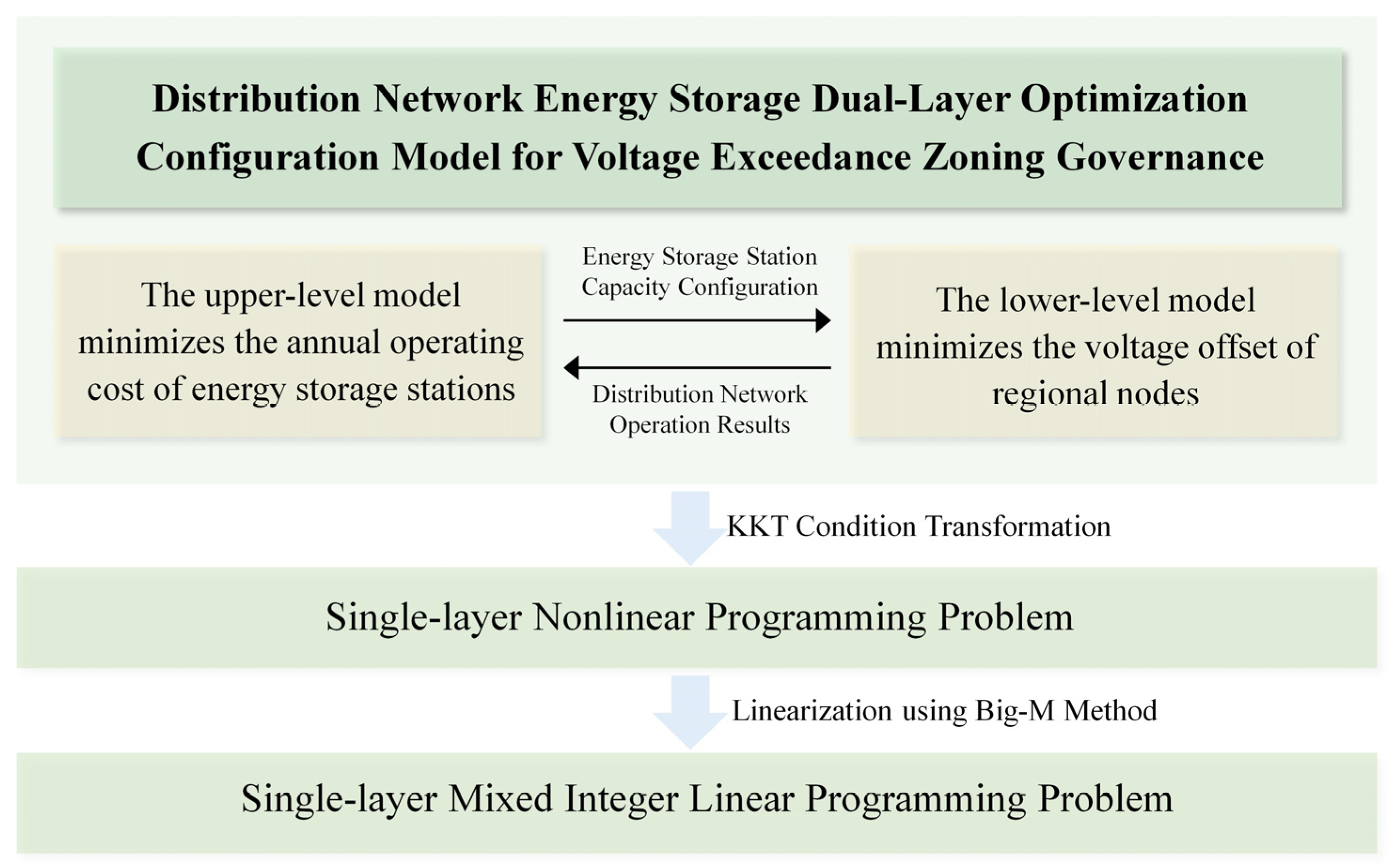
The upper-level model focuses on planning the configuration with the optimal annual operating costs of the energy storage power station, while the lower-level model prioritizes optimal dispatch with the minimal regional node voltage offset. This dual-level approach considers economic factors, while maximizing the effectiveness of regional voltage governance in the distribution network.

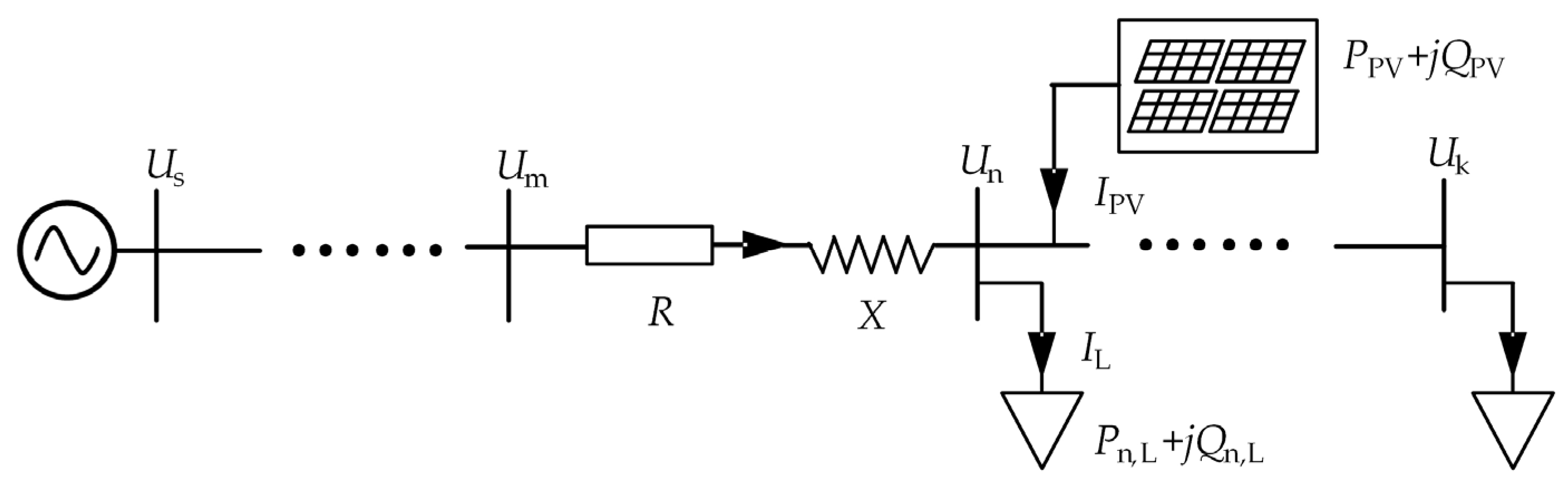
2. Operational and Regulatory Dynamics of Photovoltaic Resources in Distribution Networks

Conventional distribution networks typically adhere to a radial configuration. As depicted in Figure 1, the model illustrates the structure of photovoltaic integration into the distribution network.
Based on equivalent circuit calculations, the voltage expression at the photovoltaic grid connection point is derived as follows:
U n = U m i = n k P i , L P PV R + i = n k Q i , L Q PV X U m
where U n and U m denote the voltages of nodes n and m, respectively, and P PV and Q PV denote the active and reactive power outputs of the photovoltaic system, respectively; R and X represent the resistance and reactance in the circuit, respectively.
From this analysis, it is evident that connecting photovoltaic systems to the grid elevates the voltage level at the connection point. When photovoltaic power output surpasses the load consumption at the grid connection point, it alters the direction of flow within the system, potentially causing voltage levels to rise and even surpass the predefined limits at the photovoltaic grid connection point. Conversely, if the grid-connected photovoltaic inverter has the capability to modulate its capacity to absorb reactive power from the distribution network or restrict the active power output of photovoltaic systems, it can effectively mitigate voltage fluctuations at the grid connection point.
Regional division is aimed at optimizing the regulatory potential of diverse resources within distribution networks, while enhancing voltage limit control across different operational scenarios. Considering the temporal and seasonal variations inherent in photovoltaic power generation, light intensity data exhibit minimal fluctuation within the same season, but vary notably across seasons. Therefore, the entire year is segmented into four seasonal time series: spring, summer, autumn, and winter, with a Beta distribution model employed for light intensity characterization [23]. By deriving probability density function parameters from historical light intensity data for each season and fitting them into a Beta distribution curve, corresponding power generation output curves can be computed using a photovoltaic power generation model.
The aggregate capacity of the photovoltaic grid-connected inverter is denoted as SN, where SDG represents the capacity utilized by grid-connected power generation, and SRE denotes the adjustable capacity, shown as follows:
S N 2 = S D G 2 + S R E 2 S D G = 3 U I 1
where U represents the voltage of the distribution network, and I1 denotes the active current output of the inverter.
Consequently, this section initially delineates operational characteristics based on the time series model of DGs, and is followed by an assessment of the adjustable regulatory resources within the distribution network capable of mitigating voltage exceedance occurrences.

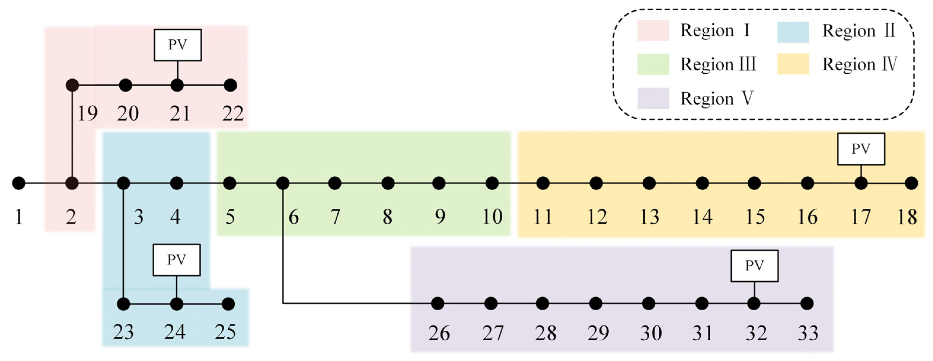
3. Voltage Partitioning Strategy Considering Distributed Photovoltaic Governance Resources

3.1. Index System for Regional Division of Distribution Network

Our research endeavored to mitigate voltage deviations and present a comprehensive indicator system that considers regional functionality. The system comprises modular indicators used to evaluate the structure of the distribution network, and voltage regulation capacity indicators aimed at enhancing voltage deviation mitigation. The overarching aim is to maximize the regional voltage governance capacity within the distribution network [24].

3.1.1. Improved Modularity Metrics

In the distribution network structure, nodes within a region exhibit tight electrical coupling, while connections between regions are more loosely integrated. This configuration facilitates the operational and managerial aspects of regional voltage control. A higher modularity index indicates a more favorable structure for the distribution network [25], as follows:
ρ = 1 2 m i j A i j k i k j 2 m δ ( i , j )
where Aij represents the edge weight between node i and node j, signifying the electrical distance between these nodes as depicted in Equations (3)–(5). m = i j A i j / 2 represents half of the total edge weights within the region. Specifically, k i = i A i j signifies the aggregate weight of all edges linked to node i. Where both node i and node j reside within the same region, δ ( i , j ) = 1 ; otherwise, δ ( i , j ) = 0 .
Given the symmetric nature of electrical distance, a logarithmic form was adopted as the mapping function, where the electrical distance is denoted as L. The magnitude of the electrical distance exhibits an inverse relationship with the degree of coupling between nodes. Increased coupling corresponds to a diminished electrical distance, indicating a closer electrical connection, as shown in the following:
A i j = 1 L i j max i , j N L i j
L i j = [ ( d i n d j n ) ] 2
d i j = lg S V P , j j + S V Q , j j S V P , i j + S V Q , i j
where SVP and SVQ represent the matrices for active and reactive voltage sensitivities in the formula, respectively. dij quantifies the extent of node j’s influence on node i, where a larger value of dij indicates a diminished impact of node j on node i, with an increased distance separating the two nodes. Lij denotes the degree of correlation between two nodes, considering the influence of other nodes within the region [26].

3.1.2. Voltage Regulation Capability Indicators

The primary challenge encountered with the large-scale integration of photovoltaics into distribution networks is when voltages exceed their limits. The voltage regulation capability index is defined as the capacity of active and reactive power, adjustable by photovoltaics, energy storage, and load resources within a given region, to regulate the maximum voltage deviation. To minimize power loss across regions, adjustments to the voltage limit should be made by optimizing the active and reactive power of internal adjustable resources within regions, based on the following:
φ V i , t = 1 , Δ V i < Δ V max i Δ V max i / Δ V i , otherwise
Δ V max i = S v p , i j Δ P max j , t + S v Q , i j Δ Q max j , t Δ P max j , t = Δ P p v j , t Δ Q max j , t = Q p v j , t
where φ V i , t represents the voltage regulation capability index of region i; n signifies the total number of nodes within the region; Δ V i denotes the voltage deviation of node i with the maximum voltage deviation observed at the highest node in the region; Δ V max i signifies the maximum voltage regulation amount of node i, accounting for the active and reactive power margin within the region; and Δ P p v j , t and Q p v j , t denote the active and reactive powers of node j’s photovoltaic at time t, respectively.

3.2. Voltage Comprehensive Zoning Index

In light of the aforementioned regional division indicators within the distribution network and a comprehensive assessment of the regulatory capacity of existing governance resources within each region, coupled with an analysis of the voltage limit zoning governance characteristics, this article proposes the following formulation of comprehensive zoning indicators for the distribution network:
σ = ( 1 τ ) ρ + τ φ V
where τ denotes the weight coefficient.
Initially, the source load prediction data are utilized to compute the power flow within the distribution network. Subsequently, considering the instances of voltages exceeding their limits, the index weight is computed to formulate the comprehensive zoning index for the distribution network, as follows:
τ = 1 N i = 1 N U i ( t ) U i * ( t ) U i , max ( t ) U i , min ( t )
where N represents the number of distribution network nodes; Ui(t) signifies the voltage of node i; Ui, max(t) denotes the upper voltage limit value of node i; Ui, min(t) represents the lower voltage limit value of node i; and U i * ( t ) denotes the voltage rating of node i.
In addressing the challenge of excessive voltages resulting from high photovoltaic penetration rates in distribution networks, the strategic selection of energy storage power station locations is paramount. This study designates photovoltaic grid connection points as pivotal nodes, and strategically situates energy storage power stations around them to effectively mitigate photovoltaic output fluctuations. This approach facilitates the absorption of surplus electrical energy to curb voltage escalation, as well as the timely release of stored energy to elevate voltage levels as required.

4. A Voltage Over-limit Governance Model Based on Optimized Energy Storage Configuration

Conventional distribution networks manifest unidirectional power flow. However, the escalating penetration of photovoltaics has induced a notable surge in bidirectional power flow, leading to challenges such as overvoltage issues and an increase in discarded solar energy. Since 2020, numerous provinces in China have advocated for the integration of energy storage equipment within photovoltaic power generation projects, in order to diminish curtailment rates [27]. In response to this paradigm shift, our research, grounded in the service model of energy storage power stations, delineates a methodology involving site selection, investment, and construction of energy storage facilities within distribution networks. This framework aims to provide users with energy storage charging and discharging services while charging service fees, ensuring economic viability and fulfilling voltage regulation requisites.

4.1. Planning Model for Upper-Level Energy Storage Power Stations

The upper-level model is tasked with resolving the optimal annual operating cost conundrum pertaining to energy storage power stations over the planning horizon. The decision variables encompass the capacity configuration and maximum charging and discharging power parameters of energy storage power stations.

4.1.1. Upper-Level Model Objective Function

The primary objective of the upper optimization is to minimize the annual operational costs incurred by energy storage power stations, defined as follows:
min C = w = 1 W [ T w ( C i n v , w + C e s s , s , w C e s s , b , w C s e r v e , w ) ]
where w represents the typical number of days; Tw signifies the number of days corresponding to the w-th typical day; Cinv,w denotes the daily average investment and maintenance cost of energy storage power stations; Cess,s,w stands for the cost of purchasing electricity from microgrids for each typical daily energy storage power station; Cess,b,w represents the cost of selling electricity to the microgrid for each typical daily energy storage power station; and Cserve,w denotes the service fee for each typical daily energy storage power station.
(i) The daily average investment and maintenance cost of energy storage power stations is defined as follows:
C inv , w = η P P ess max + η S E ess max T s + M ess
where η P and η S represent the power cost and capacity cost of the energy storage power station, measured in CNY/kW and CNY/(kW·h), respectively, while P ess max and E ess max denote the maximum charging and discharging power and the maximum capacity of the energy storage power station, respectively. Additionally, Ts stands for the expected usage days of the energy storage power station, and Mess denotes the daily maintenance cost.
(ii) The expenditure associated with procuring electricity from the distribution network for each typical daily energy storage power station is defined as follows:
C e s s , s , w = i = 1 N t = 1 N T [ δ ( t ) P e s s , s , w , i ( t ) Δ t ]
where N represents the number of microgrids; NT signifies the number of scheduling cycle periods; δ ( t ) denotes the electricity price at which the microgrid sells electricity to energy storage stations during time period t; Pess,s,w,i(t) represents the power sold to the energy storage station during the i-th microgrid time period of each typical day; and Δ t is the scheduling period.
(iii) The revenue derived from the sale of electricity to the distribution network for each typical daily energy storage power station is defined as follows:
C ess , b , w = i = 1 N t = 1 N T λ ( t ) P ess , b , w , i ( t ) Δ t
where λ(t) signifies the electricity price for purchasing electricity from energy storage power stations for the microgrid during time period t, and Pess,b,w,i(t) represents the power purchased from the energy storage power station during the i-th microgrid time period of each typical day.
(iv) The service fee levied by each typical daily energy storage power station on the microgrid is defined as follows:
C serve , w = i = 1 N t = 1 N T θ ( t ) P ess , b , w , i ( t ) + P ess , s , w i ( t ) Δ t
where θ ( t ) represents the unit price of the service fee paid by the microgrid to the energy storage power station during time t, measured in CNY/(kW·h).

4.1.2. Upper-Level Model Constraints

(i) Capacity constraints for energy storage power stations are delineated by their rated power, as elucidated in reference [28]. Specifically, the capacity of energy storage power stations exhibits a direct proportionality to their rated power, as follows:
E e s s max = β P e s s max
where β represents the energy multiplier for energy storage power stations.
(ii) The state of charge for energy storage power stations, as well as the constraints on charging and discharging power, are as follows:
E ess ( t ) = E ess ( t 1 ) + η a b s P ess , abs ( t ) 1 η r e l e a P ess , relea ( t ) Δ t E ess ( 0 ) = 20 % E ess max 10 % E e s s max E ess ( t ) 90 % E e s s max 0 P ess , abs ( t ) U a b s ( t ) P e s s max 0 P ess , relea ( t ) U r e l e a ( t ) P e s s max U a b s ( t ) + U r e l e a ( t ) 1 U a b s ( t ) 0 , 1 , U r e l e a ( t ) 0 , 1
where Eess(t) represents the energy stored in the energy storage power station; η a b s and η r e l e a denote the charging and discharging efficiencies of the energy storage device, respectively; Pess,abs(t) and Pess,relea(t) signify the charging and discharging powers of the energy storage power station, respectively; Eess(0) is the initial stored energy of the energy storage power station; and Uabs(t) and Urelea(t) are the charging and discharging status bits of the energy storage power station, respectively, which are 0–1 variables.

4.2. Voltage Optimization Model for Lower-Level Areas

Analysis of the lower-level areas involves optimizing the steady-state operation and scheduling of photovoltaic and energy storage active control systems. An optimization model was constructed that focuses on minimizing voltage offsets at regional nodes to enhance the capacity for new energy consumption, mitigates grid losses, and enhances power quality. This model was tasked with optimizing operation to minimize voltage offsets at regional nodes. Its decision variables encompass the following: branch current, node voltage, active and reactive power at the head end of branch ij, active and reactive power injected into node j by photovoltaic sources, power purchased from the power grid, power procured from energy storage stations by the distribution network, and power sold from microgrids to energy storage stations.

4.2.1. Lower-Level Model Objective Function

The lower-level objective function minimizes the voltage offset of each regional node in the distribution network based on the participation of photovoltaic and energy storage power stations, as follows:
min C = w = 1 W t = 1 N T i = 1 N T W Δ t U w , t , i 2 ( t ) 1
where Uw,i(t) represents the voltage standard value of node i in the w-th typical day period.

4.2.2. Lower-Level Model Constraints

(i) The power balance constraints are as follows:
i a k ( j ) ( P w , ij ( t ) l w , ij r ij ) + P grid , w , j ( t ) + P pv , w , j ( t ) + P ess , b , w ( t ) P ess , s , w ( t ) P load , w , j ( t ) = i c k ( j ) P w , jm ( t ) : λ 1 , t , w i a k ( j ) ( Q w , ij ( t ) l w , ij x ij ) + Q grid , w , j ( t ) + Q pv , w , j ( t ) + Q ess , b , w ( t ) Q ess , s , w ( t ) Q load , w , j ( t ) = i c k ( j ) Q w , jm ( t ) : λ 2 , t , w
where ak(j) denotes the set of starting points of all branches in distribution network area k with j as the endpoint, ck(j) represents the set of endpoints of all branches in distribution network area k with j as the starting endpoint. Pw,ij(t), Pw,jm(t), Qw,ij(t), and Qw,jm(t) signify the active and reactive power at the head end of branches ij and jm during typical daily period t of w, respectively. lw,ij represents the square of the current amplitude of branch ij. rij and xij denote the resistance and reactance of branch ij, respectively. Pgrid,w,j(t) and Qgrid,w,j(t) denote the active and reactive power injected into node j of the power grid during typical daily period t of w, respectively. Ppv,w,j(t) and Qpv,w,j(t) represent the active and reactive power injected by photovoltaic at node j, and Pload,w,j(t) and Qload,w,j(t) denote the active and reactive power of node j’s load, respectively.
(ii) The power flow constraint is as follows:
2 P w , ij 2 P w , ij l w , ij u w , i T 2 l w , ij + u w , i
where relaxation parameters u w , i ( t ) = U w , i 2 ( t ) and l w , ij ( t ) = I w , ij 2 ( t ) are involved.
(iii) The node voltage and branch current constraints are shown as follows:
u w , j ( t ) = u w , i ( t ) 2 ( r ij P w , ij ( t ) + x ij Q w , ij ( t ) ) + ( r ij 2 + x ij 2 ) l w , ij ( t ) : λ 3 , t , w
( U w , i min ) 2 u w , i ( t ) ( U w , i max ) 2 : μ 1 , t , w min , μ 1 , t , w max 0 l w , ij ( t ) ( I w , ij max ) 2 : μ 2 , t , w min , μ 2 , t , w max
where U w , i max and U w , i min represent the maximum and minimum voltage amplitudes of node i during the typical day t period of w, respectively. According to the national standard 10 kV voltage deviation limit of 7%, it can be seen that they are 1.07 and 0.93, respectively; and I w , ij max denotes the safe current of branch ij during the typical day t period of w.
(iv) The constraints on the upper and lower limits of photovoltaic output are the following:
P pv min P pv , w , i ( t ) P pv max : μ 3 , t , w min , μ 3 , t , w max Q pv min Q pv , w , i ( t ) Q pv max : μ 4 , t , w min , μ 4 , t , w max ( P pv max ) 2 + ( Q pv max ) 2 = S pv max
where P pv max , P pv min , Q pv max , and Q pv min denote the upper and lower limits of the active and reactive power outputs of the photovoltaic system, respectively, while S pv max represents the total capacity of the photovoltaic grid-connected inverter.
(v) The power balance constraints for charging and discharging of energy storage power stations are the following:
P ess , b , w ( t ) P ess , s , w ( t ) = P ess , realea ( t ) P ess , abs ( t ) : λ 4 , t , w
(vi) The power constraints for purchasing electricity from the power grid are as follows:
0 P grid , w ( t ) P grid , mg max : μ 5 , t , w min , μ 5 , t , w max
where P grid , mg max represents the maximum power purchased by the distribution network from the power grid.
(vii) The power purchase and sale constraints between low-voltage distribution networks and energy storage power stations are represented as follows:
0 P ess , s , w ( t ) P ess , mg max : μ 6 , t , w min , μ 6 , t , w max 0 P ess , b , w ( t ) P ess , mg max : μ 7 , t , w min , μ 7 , t , w max U buy , w ( t ) + U sale , w ( t ) 1 : μ 8 , t , w min , μ 8 , t , w max
where P ess , mg max represents the maximum interaction power between the distribution network and the energy storage power station, while Ubuy,w(t) and Usale,w(t) denote the purchasing and selling statuses of electricity between each typical day and the energy storage power station. The variables λ1,t,w, λ2,t,w, λ3,t,w, λ4,t,w, λ5,t,w, λ6,t,w, λ7,t,w, and λ8,t,w denote the Lagrange multipliers associated with the equality constraints, while μ 1 , t , w min , μ 1 , t , w max , μ 2 , t , w min   μ 2 , t , w max , μ 3 , t , w min , μ 3 , t , w max , μ 4 , t , w min , μ 4 , t , w max , μ 5 , t , w min , μ 5 , t , w max , μ 6 , t , w min , μ 6 , t , w max , μ 7 , t , w min , μ 7 , t , w max , μ 8 , t , w min , and μ 8 , t , w max denote the Lagrange multipliers corresponding to the inequality constraints.

4.3. Voltage Optimization Model for Lower-Level Areas

Figure 2 illustrates the solution methodology employed in this study. The proposed two-layer model encompasses upper-level integer variables, continuous variables, and nonlinear constraints. The lower-level areas pose a challenge as they involve a mixed-integer linear programming problem that is not directly solvable. To address this, a Lagrangian function was established for the lower-level model, and then transformed into a constraint for the upper-level model, leveraging KKT complementary relaxation conditions. This transformation converts the lower-level model into a single-layer nonlinear model. The Big-M method is applied to linearize the nonlinear term, resulting in a mixed-integer linear programming problem [24]. For modeling, the YALMIP toolkit was utilized, and the Gurobi solver was invoked for solving purposes.
To elaborate, construction of the Lagrangian function Equation (27) for the lower model was delineated. Subsequently, leveraging of the constructed Lagrangian function (27) was carried out, alongside the KKT complementary relaxation condition of the lower-layer model and the additional constraints (A3) and (A4) for the upper-layer model. The resulting transformed single-layer model is presented in Equations (A1)–(A4) in Appendix A, where (A1) and (A2) denote the optimization objectives and constraints of the original upper model.
L = w = 1 W i = 1 N t = 1 N T T W Δ t ( U w , i ( t ) 1 ) 2 + λ 1 , t , w [ i a k ( j ) ( P w , ij ( t ) l w , ij r w , ij ) + P grid , w , j ( t ) + P pv , w , j ( t ) + P ess , b , w ( t ) P ess , s , w ( t ) P load , w , j ( t ) i c k ( j ) P w , jm ( t ) ] + λ 2 , t , w [ i a k ( j ) ( Q w , ij ( t ) l w , ij x w , ij ) + Q grid , w , j ( t ) + Q pv , w , j ( t ) + Q ess , b , w ( t ) Q ess , s , w ( t ) Q load , w , j ( t ) i c k ( j ) Q w , jm ( t ) ] + λ 3 , t , w [ u w , i ( t ) u w , j ( t ) 2 ( r ij P w , ij ( t ) + x ij Q w , ij ( t ) ) + ( r ij 2 + x ij 2 ) l w , ij ( t ) ] + λ 4 , t , w ( P ess , b , w ( t ) P ess , s , w ( t ) P ess , realea ( t ) + P ess , abs ( t ) ) + μ 1 , t , w min ( ( U w , i min ) 2 u w , i ( t ) ) + μ 1 , t , w max ( u w , i ( t ) ( U w , i max ) 2 ) μ 2 , t , w min l w , ij ( t ) + μ 2 , t , w max ( l w , ij ( t ) ( I w , i max ) 2 ) + μ 3 , t , w min ( P pv min P pv , w , i ( t ) ) + μ 3 , t , w max ( P pv , w , i ( t ) P pv max ) + μ 4 , t , w min ( Q pv min Q pv , w , i ( t ) ) + μ 4 , t , w max ( Q pv , w , i ( t ) Q pv max ) μ 5 , t , w min P grid , w ( t ) + μ 5 , t , w max ( P grid , w ( t ) P grid , mg max ) μ 6 , t , w min P ess , s , w ( t ) + μ 6 , t , w max ( P ess , s , w ( t ) P ess , mg max U sale , w ( t ) ) μ 7 , t , w min P ess , b , w ( t ) + μ 7 , t , w max ( P ess , b , w ( t ) P ess , mg max U buy , w ( t ) ) + μ 8 , t , w max ( U buy , w ( t ) + U sale , w ( t ) 1 )

5. Case Study

This study employed the IEEE-33 nodes for analysis, with the system composition and detailed parameters outlined in reference [29]. As the distributed power grid attains uniform power quality levels, nodes with higher load levels at the termini of each branch accommodate larger allowable power capacities for connection. Consequently, nodes 17, 21, 24, and 32, characterized by elevated load levels, were selected as access points for the photovoltaic system.
The network voltage level in this study was set at 10 kV. The photovoltaic system’s unit power in the calculation example corresponds to typical daily output, and the distribution network connects to the external power grid via node 1. Market price fluctuations in electricity were disregarded in this analysis. The electricity purchase price from the power grid followed the ordinary user time-of-use electricity price in Jiangsu Province, while the purchase and sale electricity prices between the distribution network and energy storage power stations are detailed in reference [30], and are shown in Table 1. The service fee paid by the distribution network for energy storage power station services was set at CNY 0.05/(kW h). The charging and discharging efficiencies of the energy storage power station were 0.95, with an operating range for stored energy between 10% and 90%, and an initial stored energy of 20%. The capacity cost of an energy storage power station was based on the average bid price of a lithium iron phosphate battery in a specific energy storage project, which amounted to CNY 1897/(kW h), along with a power cost of CNY 1000/kW and an operation and maintenance cost of CNY 72/(year kW) [31]. The service life expectancy of the energy storage power station was set at 8 years.
Figure 3 depicts the active power curves of photovoltaic units at nodes 17, 21, 24, and 32 on typical days of different seasons, with a time granularity of 15 min. Typical solar energy and distribution network load forecasting data for summer were selected and combined with power flow calculations to predict the operating state of the distribution network, and to determine the voltage variations at each node. Based on the aforementioned process, an assessment of the voltage levels in the distribution network was conducted, thereby delineating the voltage zones within the distribution network. Table 2 shows the photovoltaic capacities at each grid-connected node.
Significantly, during peak afternoon power generation from photovoltaic sources, a notable voltage exceedances were observed at the termini of the distribution network line, particularly at nodes 17 and 18. Conversely, during the evening peak load period, instances of voltages exceeding their limits diminished. The distribution network’s voltage levels at different time intervals are illustrated in Figure 4. Based on Equation (9), computed with an index weight of 0.691 derived from the voltage level of each node within the distribution network, the comprehensive zoning index of the distribution network was established, resulting in a division of the distribution network areas illustrated in Figure 5.
Figure 5 illustrates the comprehensive division of the distribution network into five regions. Region III, lacking photovoltaic integration, maintains a satisfactory voltage level without requiring additional adjustment resources. In contrast, Regions I, II, IV, and V experience photovoltaic power injection impacts at their terminal ends, resulting in varying degrees of voltage deviation.
As depicted in Figure 6, regions IV and V exhibit relatively substantial voltage fluctuations, manifesting voltage exceedances during peak noon periods. Notably, nodes 17 and 32 display the most pronounced overvoltage, with peak voltage fluctuations exceeding 8%. Consequently, energy storage power stations were strategically positioned at these junctures to facilitate on-site consumption of photovoltaic power within the region. Meanwhile, other regions rely on photovoltaic governance resources to enhance the self-sufficiency of each distribution network region across various operational scenarios, thus optimizing regional voltage control.
Utilizing a dual-layer configuration model, the upper objective function determined the upper limit of energy storage capacity to be 2.5 MW. The total configuration cost of energy storage amounted to CNY 12.248 million, with an annual income of CNY 2.316 million, indicating promising potential for profitability. To facilitate observations of the energy storage’s timing actions, one typical day’s energy storage activity was selected to elucidate the pressure regulation process. The temporal output behavior of node 17’s energy storage is depicted in Figure 7. Negative values denote energy storage discharge, while positive values denote energy storage charging. The graph illustrates energy storage charging during peak photovoltaic output and discharging during off-peak periods, effectively facilitating peak shaving and valley filling. Between 08:00 and 17:00, energy storage is charged to counteract any node overvoltage attributed to distributed photovoltaic output, aligning with the region’s power consumption requirements during this timeframe. Conversely, during 00:00–07:00 and 18:00–24:00, when distributed photovoltaics exhibit minimal or no output, energy storage discharges to meet power demands during peak load intervals. Moreover, to balance state-of-charge (SOC), energy storage is discharged to mitigate reliance on main grid power.
When the energy storage configuration and photovoltaic output are optimally connected to the grid for voltage regulation, the voltage amplitudes at each grid-connected node result, as illustrated in Figure 7. After energy storage was implemented, notable enhancements in the voltage levels were observed at nodes 17 and 32. Additionally, nodes 21 and 24, initially exhibiting high voltage amplitudes, experienced voltage deviation reductions, and the power quality improved through the integration of adjustable-capacity photovoltaics into the governance strategies. Notably, before and after energy storage integration into the distribution network, negligible variation resulted in the voltage levels of each node within Region III, underscoring the imperative of power quality considerations while endeavoring to ensure sustained high voltage levels across diverse time periods.
Table 3 illustrates that nodes 17 and 21 exhibit relatively high voltage fluctuations due to their substantial grid-connected capacities, with similar fluctuation values. Despite node 32 having a smaller grid-connected capacity compared to node 24, its voltage fluctuations remained higher. Analysis of the network architecture diagram reveals that node 32 is distant from the distribution network bus, resulting in higher total line impedance and increased voltage fluctuation. At 2.875%, its peak voltage fluctuation meets national standards. The lower-level model minimizes regional voltage deviations, further limiting grid voltage amplitudes and enhancing the voltage quality at each grid-connected node. Node 17 experienced a maximum voltage deviation of 3.264%, which is 7% below the 10 kV grid deviation limit. Figure 8 illustrates typical intraday voltage fluctuations post-governance across different regions, indicating the efficacy of the optimized control strategy. This strategy optimally absorbs required power within regions, leading to reduced voltage fluctuations in each area.
Through a comparative analysis of the voltage quality at grid-connected points, the peak voltage fluctuations observed at each grid-connected node under the proposed algorithm surpassed those of both traditional voltage regulation methods and the accurate model algorithm outlined in study [28], as illustrated in Table 3. Furthermore, when considering similar economic costs associated with global energy storage configurations, a detailed examination of voltage fluctuations across different regions reveals a notable enhancement in regional voltage by 28.7% through the approach presented in this paper. This finding underscores the superior voltage regulation efficacy achieved by the optimized double-layer energy storage configuration algorithm proposed herein.

6. Conclusions

This study investigated a distribution network with a high penetration rate of photovoltaics, and proposed a two-layer optimal allocation method for distribution network energy storage based on voltage zoning governance. Specifically, the upper-level model focuses on planning the configuration based on the optimal annual operating cost of the energy storage power station, while the lower-level model focuses on optimizing dispatch with the smallest regional node voltage offset. To bridge these layers, the lower-level model was transformed into the constraint conditions of the upper-level model using KKT conditions, and the Big-M method was employed to linearize the nonlinear model into a mixed-integer linear programming problem. Through simulation verification, the following conclusions were drawn:
(i)
A distribution network regional division index system was proposed, incorporating a modularity index considering the distribution network grid structure and a voltage regulation capability index to address voltage deviations. This system utilized existing governance resource regulation capacities within the region, coupled with voltage over-limit zoning governance, to obtain the comprehensive zoning index of the distribution network.
(ii)
Photovoltaic governance resources were shown to enhance the autonomy of each distribution network region under different operating scenarios. Energy storage, configured at grid connection points, enables 100% local consumption of photovoltaic power in the region, and better serves regional voltage control through the coordination of active and reactive power.
(iii)
The double-layer optimal configuration model accounted for the planned configuration of energy storage power stations and optimized dispatch of regional voltages. Case analysis demonstrated that the proposed strategy not only yields significant economic benefits, but also outperforms the optical storage capacity optimization model in terms of regional performance, achieving a notable 28.7% increase in voltage improvement effect.
The current study may not have comprehensively addressed all of the intricate factors and constraints present in real-world scenarios. Therefore, a promising direction for future research involves integrating electric vehicle energy storage for distribution network regulation, in order to further optimize energy storage system operations. Additionally, extending the optimal configuration methodology to larger-scale distribution network systems will be crucial to validate its applicability and effectiveness across varying scales.

Author Contributions

Conceptualization, M.H., J.L., Y.L. and L.Q.; methodology, M.H., J.L., J.W. and L.Q.; software, J.L. and L.W.; validation, Y.L. and L.Q.; formal analysis, Y.L. and J.W.; writing—original draft preparation, M.H. and L.W.; visualization, J.L. and J.W.; project administration, L.W.; investigation, Y.L.; writing—review and editing, J.W; supervision, L.Q. All authors have read and agreed to the published version of the manuscript.

Funding

State Grid Fujian Electric Power Co. Ltd. Technology Project Funding: 52130423000R.

Data Availability Statement

The original contributions presented in the study are included in the article, further inquiries can be directed to the corresponding author.

Conflicts of Interest

Authors Meimei Hao and Lianhui Wang were employed by the company State Grid Fujian Electric Power Co., Ltd.; Jinchen Lan and Yan Lin were employed by the company State Grid Fujian Electric Power Co., Ltd. Electric Power Science Research Institute. The authors declare that this study received funding from State Grid Fujian Electric Power Co., Ltd. The remaining authors declare that the research was conducted in the absence of any commercial or financial relationships that could be construed as a potential conflict of interest.

Appendix A

Appendix A.1

min C = w = 1 W [ T w ( C i n v , w + C e s s , s , w C e s s , b , w C s e r v e , w ) ]
E e s s max = β P e s s max E ess ( t ) = E ess ( t 1 ) + η a b s P ess , abs ( t ) 1 η r e l e a P ess , relea ( t ) Δ t E ess ( 0 ) = 20 % E ess max 10 % E e s s max E ess ( t ) 90 % E e s s max 0 P ess , abs ( t ) U a b s ( t ) P e s s max 0 P ess , relea ( t ) U r e l e a ( t ) P e s s max U a b s ( t ) + U r e l e a ( t ) 1 U a b s ( t ) 0 , 1 , U r e l e a ( t ) 0 , 1
λ 1 , t , w 2 λ 3 , t , w r ij 2 λ 6 , t , w = 0 λ 2 , t , w 2 λ 3 , t , w x ij 2 λ 6 , t , w = 0 λ 1 , t , w μ 3 , t , w min + μ 3 , t , w max = 0 λ 2 , t , w μ 4 , t , w min + μ 4 , t , w max = 0 λ 1 , t , w r w , ij λ 2 , t , w x w , ij + λ 3 , t , w ( r ij 2 + x ij 2 ) + λ 4 , t , w + λ 5 , t , w + μ 2 , t , w max = 0   T W + λ 3 , t , w λ 4 , t , w + λ 5 , t , w μ 1 , t , w min + μ 1 , t , w max = 0   μ 5 , t , w min + μ 5 , t , w max = 0 λ 1 , t , w μ 7 , t , w min + μ 7 , t , w max = 0 λ 1 , t , w μ 6 , t , w min + μ 6 , t , w max = 0 μ 7 , t , w max P ess , mg max + μ 8 , t , w max = 0 μ 6 , t , w max P ess , mg max + μ 8 , t , w max = 0 λ 4 , t , w + λ 6 , t , w = 0
0 μ 1 , t , w min ( u w , i ( t ) ( U w , i min ) 2 ) 0 0 μ 1 , t , w max ( ( U w , i max ) 2 u w , i ( t ) ) 0 0 μ 2 , t , w min l w , ij ( t ) 0 0 μ 2 , t , w max ( ( I w , i max ) 2 l w , ij ( t ) ) 0 0 μ 3 , t , w min ( P pv , w , i ( t ) P pv min ) 0 0 μ 3 , t , w max ( P pv max P pv , w , i ( t ) ) 0 0 μ 4 , t , w min ( Q pv , w , i ( t ) Q pv min ) 0 0 μ 4 , t , w max ( Q pv max Q pv , w , i ( t ) ) 0 0 μ 5 , t , w min P grid , w ( t ) 0 0 μ 5 , t , w max ( P grid , mg max P grid , w ( t ) ) 0 0 μ 6 , t , w min P ess , s , w ( t ) 0 0 μ 6 , t , w max ( P ess , mg max U sale , w ( t ) P ess , s , w ( t ) ) 0 0 μ 7 , t , w min P ess , b , w ( t ) 0 0 μ 7 , t , w max ( P ess , mg max U buy , w ( t ) P ess , b , w ( t ) ) 0 0 μ 8 , t , w max ( 1 U buy , w ( t ) U sale , w ( t ) ) 0
The transformed single-layer model is represented by constraints (A1)–(A4), wherein the nonlinear constraints within constraints (A2) and (A3) are reformulated using the Big-M method. This involves the introduction of several 0–1 variables to linearize the original nonlinear constraints. For instance, let us consider the conversion of the first equation in constraint (A4) into constraint (A5). We elucidate this process as follows, noting that the conversion methodology for other constraints follows a similar approach [24]:
0 μ 1 , t , w min M v 1 , t , w min 0 u w , i ( t ) ( U w , i min ) 2 M ( 1 v 1 , t , w min )
where M represents a sufficiently large constant, and v 1 , t , w min denotes a binary variable.

Appendix A.2

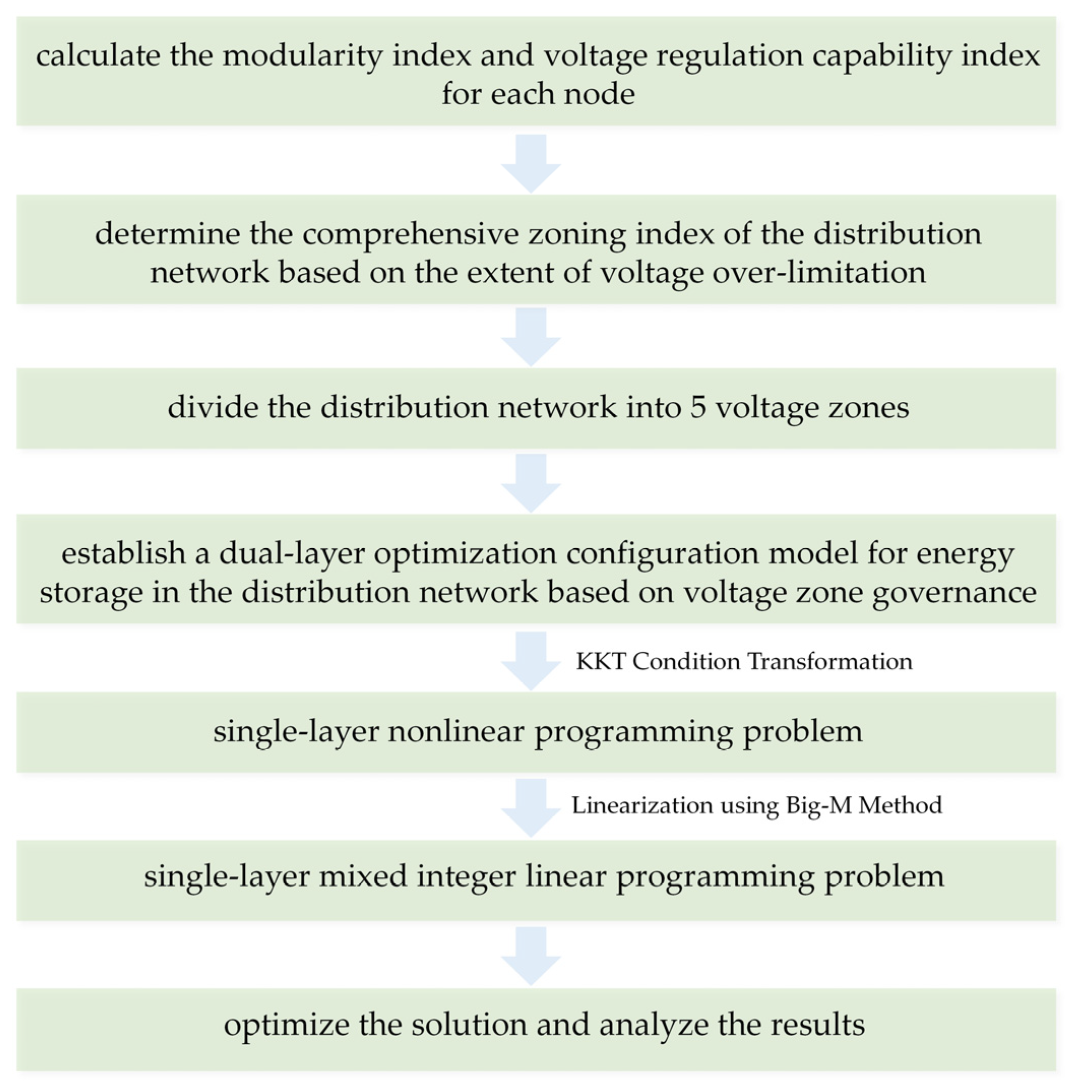
Algorithm A1: Voltage Partitioning Algorithm and Dual-Layer Energy Storage Configuration Model
Regional partitioning algorithm:
  RG = initPartition(); CMG = 0; %Initialize each node as its own community
1: while CMG > 0
2: For v in G %For each node v in G
3: For w of v %For each neighbor w of v
4: CMG = CMG(v, w);
    %Calculate the modularity gain of v after moving to the community of w
5: VRC = VRC(v, w);
    %Calculate the voltage regulation ability of v after moving to community w
6: vlacation = (1 − w) * CMG + w * VRC; %Determine comprehensive indicators based on weights
7: v = v + 1;
8: end
9: end
10: end
11: print(Partition (Region G))

Double-layer optimization model:
1: min Cost(x); %Upper-Level Model Objective Function
2: subject to: Constraints(x, y); % Upper-Level Model Constraints
3: min VoltageDeviation(y); % Lower-Level Model Objective Function
4: subject to: Constraints(y); % Lower-Level Model Constraints
5: y = argmin{VoltageDevia tion(y)};
6: SNLP = KKT(LM); %KKT transforms the lower-level model into a constraint condition for the upper-level model, making it a single-layer nonlinear model
7: SMILP = BigM(SNLP); %The Big-M method linearizes the nonlinear terms in the transformed single-layer nonlinear model
8: print(optimization)
Figure A1. Flowchart of the strategy proposed in this paper.
Energies 17 01847 g0a1

References

  1. Liu, J.L.; Liu, X.M.; Lu, X. Analysis Method and Countermeasures for Supply-Demand Balance of High Proportion New Energy Systems. High Volt. Eng. 2023, 49, 2711–2724. [Google Scholar]
  2. Chen, X.L.; Sun, J.; Zhang, J.L.; Lv, Q.Y. Intelligent Switch Location Strategy of Distribution Network Smart Switch Based on New Energy Consumption and User-Side Response Master-Slave Game. Electr. Power Autom. Equip. 2024, 44, 57–63. [Google Scholar]
  3. Liu, J.Y.; Lu, L.; Gao, H.J.; Liu, J.Y.; Shi, W.C.; Wu, Y. Active Distribution Network Planning Considering Characteristics of Distributed Power Sources and Electric Vehicles. Autom. Electr. Power Syst. 2020, 44, 41–48. [Google Scholar]
  4. Chen, Z.; Sun, Y.; Zhang, Y.; Li, M.C.; Zhang, D.L.; Xiao, W. Study on Optimized Configuration of Energy Storage Considering Wind-Solar Complementarity. Trans. China Electrotech. Soc. 2021, 36, 145–153. [Google Scholar]
  5. Li, C.P.; Dong, Z.M.; Li, J.H.; Li, H.J.; Zhou, H.Y.; Jin, Q. Optimization Control Strategy of Distributed Energy Storage Cluster to Improve New Energy Consumption Capacity of Distribution Network. Autom. Electr. Power Syst. 2021, 45, 76–83. [Google Scholar]
  6. Zhao, Y.; Wu, Z.; Qian, Z.; Gu, W.; Li, D.; Liu, Y. Distributed Optimization Scheduling of Active Distribution Network Considering Spatial and Temporal Correlation of Load and Generation. Autom. Electr. Power Syst. 2019, 43, 68–76. [Google Scholar]
  7. Li, Z.; Wang, W.B.; Han, S.F. Research on Voltage Adaptability of Distributed Photovoltaic Access Distribution Network Considering Reactive Power Support. Power Syst. Prot. Control 2022, 50, 32–41. [Google Scholar] [CrossRef]
  8. Li, P.S.; Wu, Z.J.; Zhang, C.; Hu, M.Q.; Wang, F.S. Distributed Mixed Time-Scale Reactive/Voltage Control for Active Distribution Network. Autom. Electr. Power Syst. 2021, 45, 160–168. [Google Scholar]
  9. Huang, W.; Liu, S.L.; Yi, Y.Q. Multi-Time-Scale Optimal Control of Distribution Network Based on Voltage Optimization of Photovoltaic Grid Connection Points. Autom. Electr. Power Syst. 2019, 43, 92–100. [Google Scholar]
  10. Huang, D.W.; Wang, X.Q.; Yu, N.; Chen, H.H. Strategy of Mixed Time-Scale Reactive/Voltage Control for Distribution Network Considering Uncertainty of Photovoltaic Output. Trans. China Electrotech. Soc. 2022, 37, 4377–4389. [Google Scholar]
  11. Yang, J.Y.; Wang, W.L.; Zhang, M.M.; Wang, L.; Zhang, Q. Voltage Stratified Control Method for Distribution Networks Considering Participation of Distributed Photovoltaics and Energy Storage. J. Electr. Power Sci. Technol. 2023, 38, 111–120+215. [Google Scholar]
  12. Yu, Z.P.; Tang, Y.; Dai, J.F.; Yi, J. Reactive Power and Voltage Control Strategy of Photovoltaic Power Station Based on Active Adaptation. Power Syst. Technol. 2020, 44, 1900–1907. [Google Scholar]
  13. Zhang, H.T.; Wei, G.; Yuan, H.T. Optimization Scheduling of DC Distribution Network Considering Hydrogen-Electric Hybrid Energy Storage. Autom. Electr. Power Syst. 2021, 45, 72–81. [Google Scholar]
  14. Zeng, X.J.; Luo, S.; Hu, X.X.; Wang, Z.; Yu, K. X. Load control and power quality monitoring of active distribution network systems. J. Electr. Power Sci. Technol. 2013, 28, 41–47. [Google Scholar]
  15. Chen, Y.; Jin, W.; Wang, W.B. Multi-Time-Scale Autonomous Strategy of Regional Energy Storage Stations Participating in Disturbance Smoothing in Distribution Network. Power Syst. Prot. Control 2021, 49, 134–143. [Google Scholar]
  16. Chen, C.L.; Li, X.L.; Ji, K.H.; Wang, Y.; Lin, S.F. Clustering and Optimization Operation of Distribution Networks Considering Matching of Source-Load-Storage. Electr. Power Constr. 2023, 44, 80–93. [Google Scholar]
  17. Shi, B.; Xiao, C.L.; Peng, K. Two-Layer Joint Expansion Planning Strategy of Distribution Network Based on Cluster Division Considering Network-Source-Storage. Autom. Electr. Power Syst. 2023, 47, 43–51. [Google Scholar]
  18. Liu, K.C.; Zhong, M.; Zeng, P.L. Review of Intelligent Reliability Assessment of Active Distribution Networks Considering Distributed Renewable Energy Sources and Energy Storage. Electr. Meas. Instrum. 2021, 58, 1–11. [Google Scholar]
  19. Wang, Z.; Wang, Y.; Liu, G.; Zhao, Y.; Cheng, Q.; Wang, C. Fast Distributed Voltage Control for PV Generation Clusters Based on Approximate Newton Method. IEEE Trans. Sustain. Energy 2021, 12, 612–622. [Google Scholar] [CrossRef]
  20. Taheri, S.I.; Davoodi, M.; Ali, M.H. A Simulated-Annealing-Quasi-Oppositional-Teaching-Learning-Based Optimization Algorithm for Distributed Generation Allocation. Computation 2023, 11, 214. [Google Scholar] [CrossRef]
  21. Chai, Y.; Guo, L.; Wang, C.; Zhao, Z.; Du, X.; Pan, J. Network Partition and Voltage Coordination Control for Distribution Networks with High Penetration of Distributed PV Units. IEEE Trans. Power Syst. 2018, 33, 3396–3407. [Google Scholar] [CrossRef]
  22. Li, C.P.; Yan, J.Q.; Sun, D.P.; Xi, X.D.; Zhang, Q. Multi-Dimensional Economic Evaluation of Distributed Energy Storage Participating in Multiple Scenarios in Distribution Network. Glob. Energy Interconnect. 2022, 5, 471–479. [Google Scholar]
  23. Li, X.J.; Sheng, X.; Yan, S.J. Distributed Collaborative Optimization of Ultra-Large-Scale Energy Storage System Based on Alternating Direction Multiplier Method. Power Syst. Technol. 2020, 44, 1681–1688. [Google Scholar]
  24. Fang, X.; Li, F.; Wei, Y.; Cui, H. Strategic Scheduling of Energy Storage for Load Serving Entities in Locational Marginal Pricing Market. IET Gener. Transm. Distrib. 2016, 10, 1258–1267. [Google Scholar] [CrossRef]
  25. Wang, J.J.; Yao, L.Z.; Liu, K.Y.; Wang, J. Dynamic Regional Division Method of Distribution Network with Regional Autonomy. Power Syst. Technol. 2024, 2, 1–12. [Google Scholar]
  26. Sun, Q.; Xu, S.; Zhu, S.Y. Distribution Network Planning Considering Time-Series Characteristics of Distributed Generation and Spatio-Temporal Characteristics of Electric Vehicles. Autom. Electr. Power Syst. 2020, 40, 30–38. [Google Scholar]
  27. Wang, Z.H.; Jia, Y.B.; Li, Y.C.; Han, X.Q. Optimization of Active Distribution Network Optical Storage Capacity Considering the Impact of Power Quality. Power Syst. Technol. 2023, 48, 607–620. [Google Scholar]
  28. Chen, L.J.; Wu, T.T.; Liu, H.B.; Huang, G.Y.; Xu, X.H. Two-Stage Large User Energy Storage Optimization Model Based on Demand Management. Autom. Electr. Power Syst. 2019, 43, 194–200. [Google Scholar]
  29. Baran, M.E.; Wu, F.F. Network Reconfiguration in Distribution Systems for Loss Reduction and Load Balancing. IEEE Power Eng. Rev. 1989, 9, 101–102. [Google Scholar] [CrossRef]
  30. Wu, S.J.; Liu, J.K.; Zhou, Q. Economic Dispatch Optimization of Cold and Heat Power Multi-Microgrid System Considering Energy Storage Station Service. Autom. Electr. Power Syst. 2019, 43, 10–18. [Google Scholar]
  31. Li, C.L.; Jia, Y.B.; Shi, J.Y.; Liu, J.J.; Han, X.Q. Frequency Regulation Capacity Allocation Strategy for Wind-Storage Systems Considering Cluster Effects of Wind Power. J. Chin. Soc. Electr. Eng. 2024, 4, 11–22. [Google Scholar]
Figure 1. Schematic diagram of photovoltaic system grid connection.
Energies 17 01847 g001
Figure 2. Model solution process diagram.
Energies 17 01847 g002
Figure 3. Active photovoltaic power output in four seasons: (a) active photovoltaic power output at nodes 17 and 21; (b) active photovoltaic power output at nodes 24 and 32.
Energies 17 01847 g003
Figure 4. Voltage diagrams of distribution network at different time intervals.
Energies 17 01847 g004
Figure 5. Division of areas in the 33-node distribution network.
Energies 17 01847 g005
Figure 6. Typical daily voltage fluctuations in each area before governance.
Energies 17 01847 g006
Figure 7. Optimization of charging and discharging behaviors of the energy storage station at node 17.
Energies 17 01847 g007
Figure 8. Typical intraday voltage fluctuation diagrams for each region after governance.
Energies 17 01847 g008
Table 1. Electricity price parameters.
PeriodElectricity Price/(CNY/(kW·h))
Price of Electricity Purchased from the GridPrice of Electricity Purchased from Energy Storage Power StationPrice of Electricity Sold to Energy Storage Power Stations
Peak08:00–12:001.361.150.95
17:00–21:00
Off-peak12:00–17:000.820.750.55
21:00–24:00
Valley00:00–08:000.370.400.20
Table 2. Photovoltaic capacities of each grid connection point.
Node Number17212432
Photovoltaic Capacity/MW1.51.511
Table 3. The peak voltage fluctuations at different grid-connected nodes under various algorithms.
StrategyNode Number
17212432
The algorithm proposed in this paper3.26%3.15%2.03%2.88%
Conventional voltage regulation4.23%5.86%6.22%5.43%
Algorithm in reference [27]2.33%5.74%5.39%4.12%
Disclaimer/Publisher’s Note: The statements, opinions and data contained in all publications are solely those of the individual author(s) and contributor(s) and not of MDPI and/or the editor(s). MDPI and/or the editor(s) disclaim responsibility for any injury to people or property resulting from any ideas, methods, instructions or products referred to in the content.

