
Effect of Entrainment on the Liquid Film Behavior in Pipe Elbows

1
CNOOC Research Institute, Beijing 100028, China
2
College of Pipeline and Civil Engineering, China University of Petroleum (East China), Qingdao 266580, China
*
Author to whom correspondence should be addressed.
Energies 2024, 17(8), 1983; https://doi.org/10.3390/en17081983
Submission received: 9 March 2024
/
Revised: 8 April 2024
/
Accepted: 12 April 2024
/
Published: 22 April 2024
(This article belongs to the Topic Formation, Exploration and Development of Natural Gas Hydrate)
Abstract
:Multiphase flow entrainment in natural gas engineering significantly influences the safety and efficiency of oil companies since it affects both the flow and the heat transfer process, but its mechanisms are not fully understood. Additionally, current computational fluid dynamics (CFD) methodologies seldom consider entrainment behavioral changes in pipe elbows. In this article, a verified CFD method is used to study the entrainment behavior, mechanism, and changes in an elbow. The results show that droplet diameter in a developed annular flow follows a negative skewness distribution; as the radial distance (from the wall) increases, the fluctuation in the droplets becomes stronger, and the velocity difference between the gas and the droplets increases linearly. Turbulence bursts and vortices sucking near the wall jointly contribute to droplet entrainment. As the annular flow enters the elbow, the secondary flow promotes the film expansion to the upper and lower parts of the pipe. Droplets re-occur near the elbow exit intrados, and their size is much smaller than those in the upstream pipe. Vortices sucking under low gas velocity play an important role in this process. These findings provide guidelines for safety and flow assurance issues in natural gas production and transportation and bridge the gap between multiphase flow theory and natural gas engineering.
1. Introduction
Currently, gas-dominant multiphase flow (i.e., churn flow and annular flow) has many natural gas engineering applications. Typically, in annular flow, high-speed gas moves through the pipe center while a liquid film flows around the pipe wall [1,2,3]. In this process, the strong interaction between the gas core and liquid film shears part of the liquid roll-wave crests and leads to droplet entrainment [4]. Entrainment is critical in gas-dominant multiphase flow since it affects the mass and heat exchanges between phases as well as phase distribution and pressure drop. These changes destabilize the flow and make it hard to predict, which negatively affects the safety and flow assurance in natural gas production and transportation. Droplet entrainment characteristics are also important for developing an accurate multiphase flow model [5,6]. However, the entrainment mechanism is not fully understood, and the empirical models available are based on simplified assumptions in specific conditions that are not accurate in many cases.
Some researchers have argued that the interfacial wave instability between two phases affects droplet entrainment [7,8,9]. Depending on the liquid flow rate, two types of waves exist on the liquid film: ripple waves and disturbance waves. When the liquid flow rate is low, ripple waves (small-scale) occur, which exist for a short time and move slowly. Therefore, droplets cannot be extracted from the liquid film. For high gas and liquid flow rates, the disturbance waves (long-length) become dominant. Since disturbance waves move faster than ripple waves, their amplitude is much higher, and their lifespan is longer [10,11]. Usually, for pipelines with a small diameter, the disturbance waves occur coherently on the circumference [12]. According to the literature, high-speed gas shears off the disturbance wave crest to form droplets; then, the droplets enter the gas core [13,14]. In this process, the gas drag force, as well as gravity, deforms and stretches the crest against the retaining liquid surface tension. As a result, the liquid ligament breaks up, and the droplet enters the gas core. However, the liquid volume detached from the wave crest is not taken into consideration in this mechanism, which makes it impossible to calculate the entrainment rate.
There are many studies on liquid sampling, flow patterns, and factors that influence liquid distribution as well as erosion using both experimental and simulation methods. Some of these are summarized in Table 1.
Regarding the empirical modeling, for vertical flow, Oliemans et al. [25] developed a correlation based on their experimental database that covers a wide range of flow conditions. Later, Ishii and Mishima [26] derived a verified correlation based on the gas Weber number and the liquid Reynolds number. Researchers also studied droplet sizes entrained in the gas core and proposed correlations based on their experimental database. Most of the correlations [27,28,29] considered the Weber number (the ratio between inertia and surface forces) as a key parameter since it indicates the interaction between the external stress force and the surface forces acting on droplets, an interaction which is important for the droplet breakup mechanism and droplet size. Kolev [27] derived a correlation to calculate the droplet diameter from Kelvin–Helmholtz instability. Fore [30] put forward a modified expression to predict the volume median diameter in vertical and horizontal flows in a pipe. Ishii [31] proposed a semi-empirical correlation to estimate the average maximum droplet size for roll-wave entrainment.
Summarizing the entrainment models above, Wicks’s model and Paleev’s model are based on experimental data in horizontal annular flow, so they are unlikely to provide a precise prediction for vertical or inclined annular flow. In contrast, Oliemans’ and Ishii’s models can provide accurate entrainment in vertical annular flow (superficial gas velocities of 15 to 40 m/s, superficial liquid velocities of 0.06 to 0.2 m/s, and pipeline diameter of 6 to 32 mm) since they use a vertical annular flow database. Magrini’s experiments [32] show that Paleev’s model provides the best prediction for horizontal annular flow. For the entrained droplet size calculation, most of the correlations choose the Weber number as the key factor. Additionally, these semi-empirical correlations are based on experimental data in specific conditions, which limits their applications.
In brief, the entrainment mechanism in annular flow is not fully understood; related models and correlations are empirical and inaccurate, which limits their application in practice. Many details on droplet entrainment are not included in the current CFD methodologies available in the literature, and no studies on how entrainment affects liquid film behavior in the elbow were found.
In this article, a verified CFD method is used to study entrainment behavior in pipelines. Firstly, entrainment characteristics like droplet diameter and velocity distribution are analyzed in detail. Then, the entrainment mechanism is interpreted based on a vortex theory. Lastly, entrainment changes in elbows are studied. These detailed analyses of liquid film and droplet entrainment help to evaluate elbow safety, with elbows being sensitive to erosion as well as corrosion, and solve flow assurance problems in natural gas production and transportation.
2. Theories and Modeling
2.1. Entrainment Modeling
The correlation established by Wicks and Dukler [15] is shown below:
where is the entrainment group (unit ft3/lbf-hr); and are the mass flow rates of liquid and gas, respectively; is the critical Weber number ranging from 13 to 22; is the droplet mass flow rate; and is the pressure gradient.
The correlation developed by Paleev [16] is listed below:
where is the mixture density of the core defined as
where is the entrainment fraction; and are the density of the liquid and gas, respectively; is the dynamic viscosity of the liquid; and are the superficial liquid velocity and superficial gas velocity, respectively; and is the surface tension.
Oliemans’ model [25] is given below:
2.2. Droplet Size
The critical Weber number is the most widely used criterion to estimate the droplet size; for the condition of high density difference (droplet in gas core), the empirical value of the Weber number is 12. The expression is as follows [27]:
where is the critical Weber number, is the gas velocity, and is the droplet diameter.
For annular flow, the volume median diameter of the droplet derived by Fore [30] can be calculated using the following equation:
where is the droplet volume median diameter, and and are the gas Weber number and the gas Reynolds number, respectively.
This correlation is simple and accurate enough to predict the droplet volume median diameter in horizontal and vertical pipelines.
The semi-empirical correlation to estimate the average maximum droplet size proposed by Ishii [26] is as follows:
where is the average maximum droplet size.
3. Experimental Background
The experimental data used for liquid entrainment verification in this study were taken from Magrini [32]. In the experiment, air from the compressor and water from the tank were measured separately and then mixed to develop a horizontal annular flow in a 76.2 mm ID pipeline. Then, the fluid entered the test section after it was fully developed. The test section included two parts: the isokinetic sampling section and the film removal section. The isokinetic sampling section measured the liquid entrainment in the gas, and the film removal section determined the liquid film flow rate. Finally, the fluid flowed out of the system from the outlet.
The isokinetic sampling section included an L-shape isokinetic probe, two valves, a container, and a gas flowmeter. The probe inlet was placed against the gas flow direction so that the droplets in the gas core could enter the probe easily. The probe could be located at different positions of the pipe cross-section. Valves were applied to control the sampling rate and keep the gas velocity in both the probe and the pipeline the same. The sampled droplets were collected in the container, and the sampled gas was vented out through the flowmeter. Then, the container was weighed to calculate the entrainment.
The film removal section includes an inserted porous sleeve that allows the liquid film to pass through, and the cavity between the sleeve and outer shell is used to store the sampled liquid. When passing the film removal section, liquid film passes through the porous section and enters the cavity. The entrained droplets in the pipe center move out directly without being removed. The collected liquid is used to calculate the film flow rate.
In these experiments, the superficial gas velocity ranged from 40 m/s to 80 m/s, and the superficial liquid velocity ranged from 0.0035 m/s to 0.04 m/s. Each test lasted for 5 min. The entrainment flux at each location can be calculated as
The entrainment fraction can be calculated as
where is the entrainment flux, is the collected liquid volume, is the sample time, and is the cross-sectional area.
4. CFD Simulation
It is difficult to acquire details of the entrainment process since it is random and changes fast. Fortunately, CFD can provide abundant information about the whole domain at any specific time. For liquid entrainment simulation, a volume of fluid (VOF) model based on the Euler method is adopted, in which the interface between immiscible fluids can be obtained. The main steps in the liquid entrainment simulation are as follows: (1) solve the single set of momentum equations shared by all the phases; (2) track the volume fraction in each computational cell through the domain; (3) solve the volume fraction equation through implicit time discretization. A flow chart representing the methodology is shown in Figure 1.
4.1. Geometry
The geometry used in this investigation is shown in Figure 2. The upstream length, L, is 10D, the curvature radius of the elbow is 1.5D, and the downstream length is 3D.
4.2. Meshing
A high-quality mesh is critical for a successful simulation. Since the entrainment process occurs at the interface of the two phases near the wall, elements in this region were refined to obtain the details. Figure 3 provides the overview and cross-section details of the mesh.
It can be seen that the domain is meshed by polygonal cells. Polygonal cells can reduce the skewness, improve the parallel solver load balancing, and minimize communication by decreasing the number of partition interface cells [33]. Figure 3c shows an enlarged view of the near-wall region, where the first-layer thickness of the mesh is 20 µm and the maximum cell size is 1 mm, the growth ratio is 1.2, and the row number of the boundary is 5. The length of the cells in both circumferential and axial directions is 1 mm, and the total number of elements is 11,338,564. Since the maximum cell size is in the same order as the droplet size, this mesh can reveal detailed information during the entrainment process.
4.3. Simulation Settings and Boundary Conditions
In this study, the annular flow simulation is performed first to analyze the entrainment process in the pipeline. The settings of the simulation are shown in Table 2.
The boundary conditions of the flow simulation are shown in Table 2. Water (liquid phase) enters the pipe circumferentially along the pipe wall, and the water entrance is ring-shaped. Air (gas phase) enters the pipe in the center of the cross-section, and the shape of the air entrance is a circle. The superficial gas velocity is 24.6 m/s, and the superficial liquid velocity is 0.1 m/s; the initial values of the corresponding air and water mass flow rates are listed in Table 3, and the time step is 0.000005 s.
Once the mass flow rate difference between the inlet and outlet decreases below 0.01 kg/s and the flow state in the pipe becomes steady, the simulation can be stopped.
5. Results and Discussion
5.1. Entrainment Fraction Validation
In this section, experimental data from the literature [32] is adopted to verify the entrainment fraction in a CFD simulation. The working conditions in both experiments and simulations are the same. The superficial gas and liquid velocities are 40 m/s and 0.01 m/s, respectively. The entrainment fractions measured by isokinetic sampling and film removal methods in a vertical orientation are 0.42 and 0.51, respectively.
Based on Equations (18)–(20), the entrainment fractions calculated by Oliemans’ and Ishii’s models are 0.53 and 0.55, respectively. As for the simulation, at the position 1D before the elbow entrance, the area-weighted average void fraction of the gas core and pipe cross-section are extracted and converted to the average entrainment fraction using the following equations:
where and are the area of droplets and liquid film in the cross-section, respectively; is the area of the gas core; and are the liquid holdup of the gas core and pipe cross-section, respectively; and is the entrainment fraction calculated using CFD. The entrainment fractions calculated above use Equations (4)–(7) and are summarized in Table 4.
As shown in Table 4, the entrainment fraction measured using isokinetic sampling is smaller than that of the film removal method. Droplets adhering to the small diameter tube surface may cause this difference. As for the film removal method, the liquid collected may contain the redeposited droplets, which makes the measured value larger. Thus, the real value should be between 0.42 and 0.51. Both Oliemans’ model and Ishii’s model give larger values than the experiments, indicating that the two models are not accurate enough. The entrainment fraction predicted using CFD is 0.47, just within the range (0.42 to 0.51), so the entrainment fraction predicted with CFD is reasonable.
5.2. Entrainment Behavior in the Pipeline
After the flow simulation stops, the phase contours as well as the velocity vectors of the pipeline longitudinal section and representative cross-sections are extracted to analyze the entrainment behavior in the pipeline.
5.2.1. Entrainment Distribution
Figure 4 shows the phase distribution and velocity vector in the pipeline. It can be seen that as the upstream length increases, the gas in the pipe center moves much faster than that near the wall, the gas velocity fluctuation in the pipe becomes obvious, and the uniform liquid film starts waving and then breaks up into droplets (see Figure 4b). Then, the droplets are gradually entrained into the pipe center by the high-speed gas. When the upstream length reaches 6D, the droplet distribution seldom changes, and the entrainment process reaches dynamic equilibrium. After entering the elbow, most of the droplets hit the elbow extrados and coalesce into liquid film. Then, the film flows along the extrados side to the downstream pipe (see Figure 4c).
Representative cross-sections of the upstream pipe are extracted to reveal more information (see Figure 4d). At an upstream length of 2D, there is a film wave at the right side of the cross-section (circled). The corresponding velocity vectors indicate that a turbulence burst here contributes to the wave. When the upstream length reaches 2.4D, the film becomes discontinuous, and “liquid bridges” (circled) occur, which are also related to the turbulence bursts near the wall. As the flow develops, turbulence bursts become stronger and break the liquid bridges into droplets, and then, the droplets are entrained into the pipe center by the gas. At an upstream length beyond 6D, the droplets are distributed uniformly in the pipe cross-section. Droplet coalescence (circled) is also found in the flow at an upstream length of 7D.
Other researchers like Zahedi [34] and Farokhipour [21] also studied liquid distribution in annular flow pipelines. Zahedi [34] only reported the liquid distribution in the middle of the elbow (elbow angle = 45°), and no liquid was found at the elbow extrados; however, this seems inaccurate, because droplets carried by the gas core will hit the extrados and form a liquid film. Farokhipour’s simulation [21] showed the liquid film distribution in the elbow well, but no droplets can be observed in the figures. Compared with their studies, the simulation in this study provides more details of droplet distribution, like droplet coalescence, which can be seen as a remedy for entrainment simulation. Another difference is the grid. Other researchers use hexahedral cells in their simulations, but polygonal cells are adopted in this study to reduce skewness to obtain more accurate results. Additionally, droplet distribution and entrainment changes in the elbow are also investigated, which have not featured in other simulations.
5.2.2. Entrainment Characteristics
Further, the void fraction (area-weighted average) of the cross-sections (every 0.25D) in the upstream section is extracted and summarized in Figure 5.
It can be seen that for the upstream length of 2D, the void fraction is steady but fluctuates slightly around 0.95. As the upstream length increases to 6D, the void fraction rises to 0.978. Meanwhile, its fluctuation becomes stronger, and droplets start to take shape and enter the gas core. Then, after 6D, the void fraction becomes steady again, with its value fluctuating more vigorously between 0.978 and 0.981. It seems that for the annular liquid inlet, the liquid droplet entrainment and re-deposition process reach dynamic equilibrium when the upstream length is beyond 6D.
According to Ishii and Kataoka [5,35], for the case where the liquid is injected smoothly as a film at the inlet, the entrained fraction expression takes the form of exponential relaxation. For the case in this study, the trend of the curve in Figure 5 is also exponential relaxation, which means the CFD results here are reasonable.
Then, the droplet information (droplet number, droplet diameter, droplet velocity, and droplet position (radial distance from the wall)) in the pipeline’s longitudinal section is collected to further analyze the entrainment. Droplet diameters and positions are measured by the scale of the phase distribution contour; droplet velocity is determined by the velocity vector in the center of the droplet.
Figure 6 shows a histogram of the relationship between droplet diameter and droplet number distribution in the longitudinal section in the developed annular flow. It can be seen that the droplet number roughly follows a negative skew distribution. Most droplet diameters are distributed in a 1 mm to 2.5 mm range, and the droplet number in the range of 2 mm to 2.5 mm is the largest, while in the range of 0 to 0.5 mm, it is the smallest.
In contrast to one study [36], for the conditions of low-pressure (below 3 atm) and low-viscosity fluid (water), the droplet diameter distribution in this study is similar to the upper limit log-normal (ULLN) distribution given by Mugele and Evans [37]. The maximum size of the droplet can be calculated based on the Kelvin–Helmholtz instability and critical Weber number.
where is the maximum diameter of the droplet, and is the critical Weber number, which equals 12. For this study, the maximum diameter of the droplet calculated using this equation is 2.7 mm, which is represented by the last bar in Figure 6.
For this study, the calculated volume median diameter of the droplet is 1.1 mm, while the volume median droplet diameter predicted using CFD simulation is 1.7 mm (54.5% higher than the calculated value). Further improvement may be achieved by refining the mesh, which is limited by the current computational resources.
Figure 7 shows the relationship between the radial distance (from the wall) and the droplet diameter in a developed annular flow. As shown in this figure, the average value of all the droplet diameters is 1.81 mm. Droplet diameter fluctuates around the average value, and its amplitude increases with the radial distance.
Table 5 presents the variance distribution of droplet diameters. It can be seen that as the radial distance (from the wall) increases, the expectation of the droplet diameter varies very slightly around 1.81 mm, by less than ±0.05 mm. However, for the variance, it increases from 0.19 to 0.63. This means that the change in droplet diameter becomes increasingly unstable the closer the droplet is to the gas core. This may be because droplets closer to the pipe center are more likely to be broken up or coalesced by the gas core turbulence, which strengthens the fluctuation.
According to Kolev [27], the droplet breakup mechanism can be expressed as a balance between the external stress force and the surface force. During the breakup, external stress force tries to disrupt the droplets, while surface tension force tries to avoid droplet deformation. From the critical Weber number, Equation (11), it can be seen that the droplet diameter varies with the inverse square of the gas velocity. As the radial distance from the wall increases, the gas velocity becomes higher, so the minimum value of droplet diameter decreases. On the other hand, according to the Kelvin–Helmholtz instability, as the gas velocity increases, the gas–liquid interface becomes more unstable. Additionally, droplet diffusion becomes stronger, so droplets are more likely to coalesce, which increases the maximum droplet diameter.
Figure 8 shows velocity distribution (both gas and droplet) according to radial distance (from the wall). It can be seen that both gas and droplet velocities rise and fluctuate as radial distance increases, while the velocity difference between gas and droplets also increases, which means that the slippage becomes more obvious. Moreover, the fluctuations in both gas and droplets become stronger.
In order to clearly express the droplet slippage, the droplet slippage ratio can be calculated with the following equation.
where is the droplet slippage ratio, and is the droplet velocity. It can be found that the slippage ratio near the wall (27.3%) is smaller than that in the pipeline center (33.8%).
5.2.3. Entrainment Mechanism
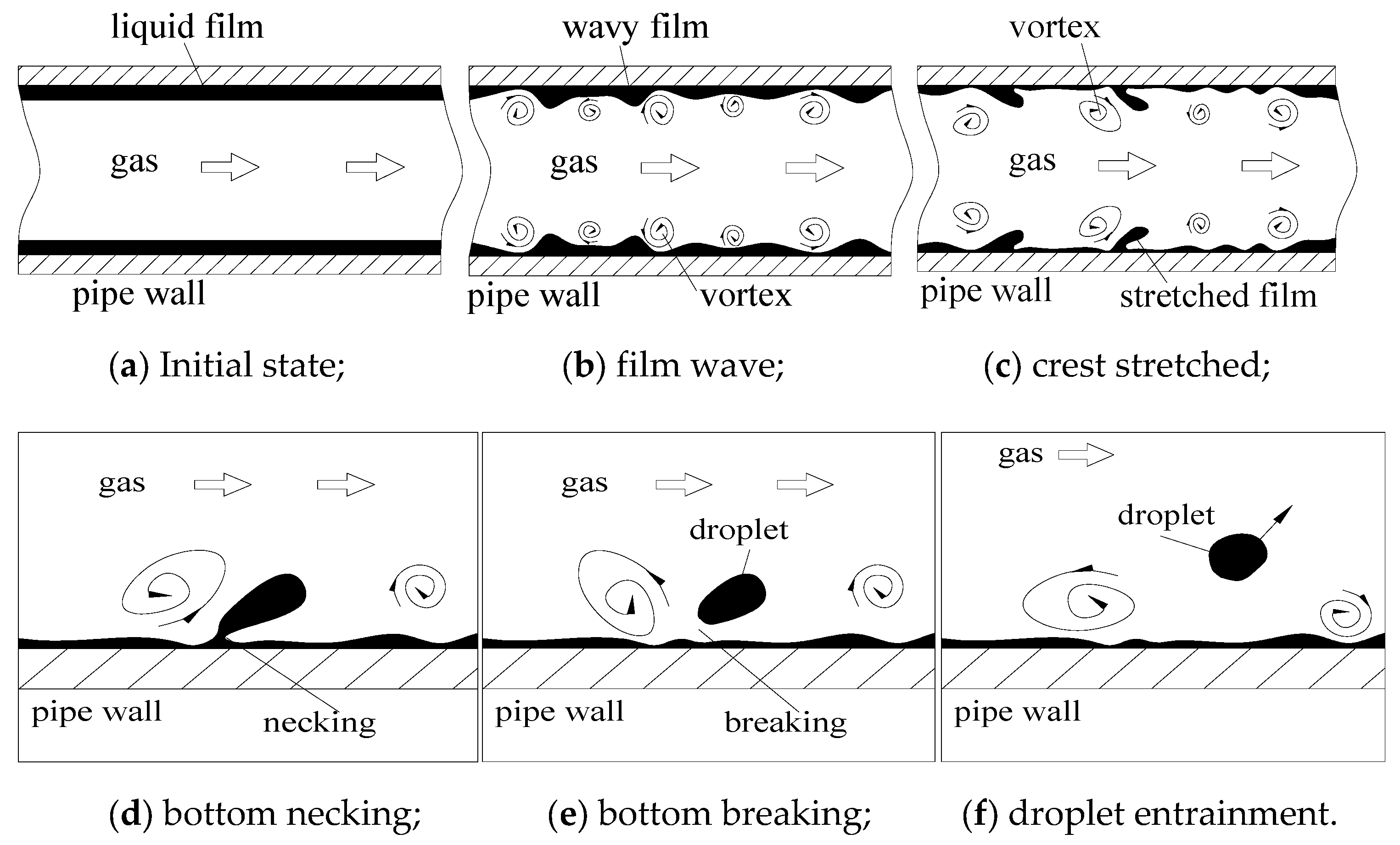
In this subsection, the mechanism of the entrainment process in annular flow is interpreted gradually, as shown in Figure 9. In the initial state (see Figure 9a), the liquid film and gas are uniform and there is no fluctuation. Since there is a velocity difference between gas and liquid film, vortices occur at the two-phase interface under the effect of shear and friction, which produce waves in the film and spread downward (see Figure 9b). As the flow develops, the crest stretched by the vortices becomes higher, and its bottom is necking under the effect of surface tension (see Figure 9c,d). Then, the necking breaks, the liquid entering the gas becomes droplets, and the rest of the liquid becomes film (see Figure 9e). The high-speed gas moving in the pipe center lowers the dynamic pressure here, so the droplets can be entrained under the pressure difference (see Figure 9f). This process reduces the film volume and makes the film discontinuous.
The Kelvin–Helmholtz instability is mainly associated with flows that have tangential variation in the velocity field [38,39,40]. This instability is caused by the hydrodynamic amplification of perturbations that arise at the gas–liquid interface with a discontinuity in the velocity field. The entrained droplet size is approximately equal to the height of the most unstable wavelength.
where is the height of the wavelength. For this study, the calculated droplet diameter is 1.8 mm, which is close to the average droplet diameter in Figure 6. This indicates that the simulation results in this study fit the Kelvin–Helmholtz instability theory and are reasonable.
As the flow develops downstream, the entrained droplets travel to the wall and are deposited into the liquid film again. As the entrainment and deposition reach dynamic equilibrium, the flow is fully developed. The most important factor that affects droplet entrainment is the vortices near the gas–liquid interface.
5.3. Entrainment Changes in the Elbow
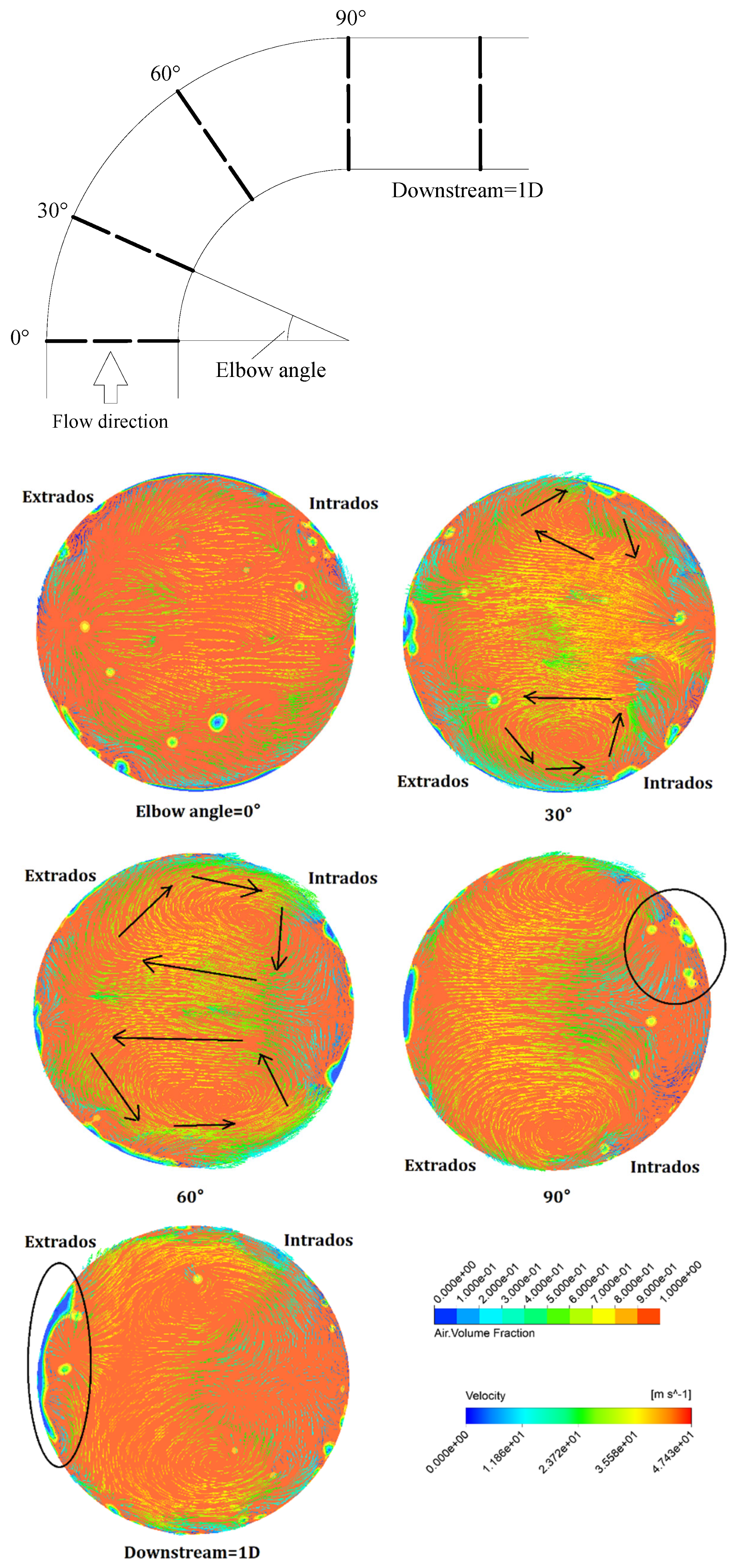
The entrainment changes when the fully developed flow enters the elbow. Figure 10 shows the phase distribution and velocity vectors of the flow in the elbow: the flow is restricted by the geometry, and the gas moves toward the elbow intrados as the flow first enters the elbow. Droplets are uniformly distributed in the pipe cross-section (elbow angle = 0°).
When the flow reaches an elbow angle of 30°, more droplets are deposited on the extrados, and the liquid film starts to take shape. The flow near the wall moves toward the intrados and forms the secondary flow. For an elbow angle of 60°, most droplets are deposited on the extrados, and droplets in the gas become less frequent, while the film becomes thicker. Two counter-rotated vortices drive the film toward the extrados. For an elbow angle of 90°, the film at the extrados thickens. Droplets occur again at the intrados under the strong effect of the vortices. After entering the downstream pipe, the film thickness at the extrados increases, and the vortices become weaker.
Unlike the roll-wave mechanism proposed by Ishii [26], which is reasonable for high gas velocity in a straight pipe, droplets re-entrained at the intrados seem to be caused by the mechanism of vortices sucking, since the gas velocity here is relatively low. As shown in Figure 4c, it is also found that the re-entrained droplet size at the intrados is smaller (1 mm–1.5 mm). This may be because vortices at the intrados provide more sucking and external stress force on the droplets for their breakup.
6. Conclusions
In this study, a verified CFD method is used to investigate entrainment behavior in a pipeline. Firstly, entrainment characteristics like droplet diameter and velocity distribution are analyzed in detail. Then, the entrainment mechanism is interpreted based on a vortex theory. Lastly, entrainment changes in the elbow are studied. The results are valuable and provide guidance for entrainment study in multiphase flow. The main conclusions are summarized below:
- (1)
- Under the annular inlet condition, the entrainment distribution along the upstream developing length from the entrance is close to a form of exponential relaxation. The droplet diameter in a developed annular flow follows a negative skewness distribution, with most droplet diameters ranging from 1.5 mm to 2 mm. As the radial distance (from the wall) increases, the fluctuation of the droplets becomes stronger, and the velocity difference between gas and droplets increases linearly.
- (2)
- Turbulence bursts and vortices near the wall jointly deform the liquid film and crest so that they begin to take shape; then, the external stress force acting on the liquid crest overcomes the surface force, and droplets form. Finally, vortices sucking transforms the droplets into gas, and the entrained droplet size is approximately equal to the height of the most unstable wavelength.
- (3)
- As the annular flow enters the elbow, droplets hit the extrados and form a liquid film, the droplet number in gas decreases, and at an elbow angle of 60°, there are no droplets in the pipe. Secondary flow promotes the film formation and expansion of the film to the upper and lower parts of the pipe. However, for an elbow angle of 90°, droplets re-occur near the elbow intrados, and the re-entrained droplet size is much smaller than that in the straight upstream pipe. Vortices sucking at low gas velocity play an important role in this process.
- Unique work description
In this study, a more accurate simulation using polygonal cells instead of hexahedral cells was carried out to investigate details of droplet distribution and entrainment changes in the elbow, which is unique and different from other simulations.
- Recommendations and future work
Although polygonal cells can provide more accurate results, they require more time and more computational resources, especially for finer grids. Grid optimization is a promising topic. In the future, AI technology like cloud computing and large data can be integrated into CFD simulations to enhance efficiency and consume fewer resources. Combined with pipeline-monitoring technologies, CFD simulation can make the detection system’s response faster and smarter.
Author Contributions
Z.X.: conceptualization, formal analysis, investigation, writing—original draft. X.C.: conceptualization, supervision. All authors have read and agreed to the published version of the manuscript.
Funding
This research was supported by the National Natural Science Foundation of China (Funding number: 51874340, Funder: Xuewen Cao).
Institutional Review Board Statement
This article does not contain any studies with human participants or animals performed by any of the authors.
Informed Consent Statement
Informed consent was obtained from all the individual participants included in the study.
Data Availability Statement
The original contributions presented in the study are included in the article, further inquiries can be directed to the corresponding authors.
Acknowledgments
The authors would like to thank Jun Zhang and the help from E/CRC at the University of Tulsa.
Conflicts of Interest
Author Zhenqiang Xie was employed by the CNOOC Research Institute, and author Xuewen Cao was employed by China University of Petroleum (East China). The remaining authors declare that the research was conducted in the absence of any commercial or financial relationships that could be construed as a potential conflict of interest.
Nomenclature
| Symbol | Description | Unit |
| Cross sectional area | m2 | |
| Area of the gas core | m2 | |
| Area of droplets on the cross-section | m2 | |
| Area of liquid film on the cross-section | m2 | |
| Pipe diameter | m | |
| Pressure gradient | MPa/m | |
| Entrainment flux | m/s | |
| Entrainment fraction | / | |
| Entrainment fraction calculated by simulation | / | |
| Gravitational acceleration | m/s2 | |
| Liquid holdup of gas core | / | |
| Liquid holdup of pipe cross-section | / | |
| Height of the wavelength | m | |
| L | Distance from the pipe inlet | m |
| Critical Weber number | / | |
| Liquid mass flow rate | kg/h | |
| Gas mass flow rate | kg/h | |
| Entrainment group | ft3/lbf-hr | |
| Gas Reynolds number | / | |
| Reynolds number of the liquid film | / | |
| Droplet slippage ratio | / | |
| Sample time | s | |
| Gas velocity | m/s | |
| Droplet velocity | m/s | |
| Collected liquid volume | m3 | |
| Critical Weber number | / | |
| Gas Weber number | / | |
| Droplet mass flow rate | kg/h | |
| Mixture density of the core | kg/m3 | |
| Gas density | kg/m3 | |
| Liquid density | kg/m3 | |
| Dynamic viscosity of liquid | Pa·s | |
| Dynamic viscosity of gas | Pa·s | |
| Superficial liquid velocity | m/s | |
| Superficial gas velocity | m/s | |
| Surface tension | N·m | |
| Droplet diameter | m | |
| Average maximum droplet size | m | |
| Droplet volume median diameter | m |
References
- Mishima, K.; Ishii, M. Flow regime transition criteria for upward two-phase flow in vertical tubes. Int. J. Heat Mass Transf. 1984, 27, 723–737. [Google Scholar]
- Wu, B.; Firouzi, M.; Mitchell, T.; Rufford, T.E.; Leonardi, C.; Towler, B. A critical review of flow maps for gas-liquid flows in vertical pipes and annuli. Chem. Eng. J. 2017, 326, 350–377. [Google Scholar] [CrossRef]
- Dasgupta, A.; Chandraker, D.K.; Kshirasagar, S.; Reddy, B.R.; Rajalakshmi, R.; Nayak, A.K.; Walker, S.P.; Vijayan, P.K.; Hewitt, G.F. Experimental investigation on dominant waves in upward air-water two-phase flow in churn and annular regime. Exp. Therm. Fluid Sci. 2017, 81, 147–163. [Google Scholar] [CrossRef]
- Ryu, S.H.; Park, G.C. A droplet entrainment model based on the force balance of an interfacial wave in two-phase annular flow. Nucl. Eng. Des. 2011, 241, 3890–3897. [Google Scholar] [CrossRef]
- Kataoka, I.; Ishii, M.; Mishima, K. Generation and size distribution of droplet in annular two-phase flow. J. Fluids Eng. 1983, 105, 230–238. [Google Scholar] [CrossRef]
- Liu, L.; Bai, B. Generalization of droplet entrainment rate correlation for annular flow considering disturbance wave properties. Chem. Eng. Sci. 2017, 164, 279–291. [Google Scholar] [CrossRef]
- Berna, C.; Escriva, A.; Munoz-Cobo, J.L.; Herranz, L.E. Review of droplet entrainment in annular flow: Interfacial waves and onset of entrainment. Prog. Nucl. Energy 2014, 74, 14–43. [Google Scholar] [CrossRef]
- Pan, L.; Hanratty, T.J. Correlation of entrainment for annular flow in horizontal pipes. Int. J. Multiph. Flow 2002, 32, 385–408. [Google Scholar] [CrossRef]
- Okawa, T.; Kotani, A.; Kataoka, I.; Natio, M. Prediction of critical heat flux in annular flow using a film flow model. J. Nucl. Sci. Technol. 2003, 40, 388–396. [Google Scholar] [CrossRef]
- Alekseenko, S.V.; Cherdantsev, A.V.; Cherdantsev, M.V.; Isaenkov, S.V.; Markovich, D.M. Study of formation and development of disturbance waves in annular gas–liquid flow. Int. J. Multiph. Flow 2015, 77, 65–75. [Google Scholar] [CrossRef]
- Schubring, D.; Shedd, T. Wave behavior in horizontal annular air-water flow. Int. J. Multiph. Flow 2008, 34, 636–646. [Google Scholar] [CrossRef]
- Belt, R.J.; Westende, J.M.C.V.; Prasser, H.M.; Portela, L.M. Time and spatially resolved measurements of interfacial waves in vertical annular flow. Int. J. Multiph. Flow 2010, 36, 570–587. [Google Scholar] [CrossRef]
- Asali, J.C.; Hanratty, T.J. Ripples generated on a liquid film at high gas velocities. Int. J. Multiph. Flow 1993, 19, 229–243. [Google Scholar] [CrossRef]
- Holowach, M.J.; Hochreiter, L.E.; Cheung, F.B. A model for droplet entrainment in heated annular flow. Int. J. Heat Fluid Flow 2002, 23, 807–822. [Google Scholar] [CrossRef]
- Wicks, M.; Duckler, A.E. Entrainment and pressure drop in concurrent gas-liquid flow: I. Air-water in horizontal flow. AIChE J. 1960, 6, 463–468. [Google Scholar] [CrossRef]
- Paleev, I.I.; Filippovich, B.S. Phenomena of liquid transfer in two-phase dispersed annular flow. Int. J. Heat Mass Tran. 1966, 9, 1089–1093. [Google Scholar] [CrossRef]
- Xu, G.; Cai, L.; Ullmann, A.; Brauner, N. Trapped water flushed by flowing oil in upward-inclined oil pipelines. In Volume 1: Upstream Pipelines; Project Management; Design and Construction; Environment; Facilities Integrity Management; Operations and Maintenance; Pipeline Automation and Measurement, Proceedings of the International Pipeline Conference, Calgary, AB, Canada, 24 September 2012; American Society of Mechanical Engineers: New York, NY, USA, 2012; pp. 637–647. [Google Scholar]
- Huang, S.; Zhang, B.; Lu, J.; Wang, D. Study on flow pattern maps in hilly-terrain air-water-oil three-phase flows. Exp Therm. Fluid Sci. 2013, 47, 158–171. [Google Scholar] [CrossRef]
- Parsi, M.; Vieira, R.E.; Torres, C.F.; Kesana, N.R.; McLaury, B.S.; Shirazi, S.A. Experimental investigation of interfacial structures within churn flow using a dual wire-mesh sensor. Int. J. Multiph. Flow 2015, 73, 155–170. [Google Scholar] [CrossRef]
- Magnini, M.; Ullmann, A.; Brauner, N.; Thome, J.R. Numerical study of water displacement from the elbow of an inclined oil pipeline. J. Petrol. Sci. Eng. 2018, 166, 1000–1017. [Google Scholar] [CrossRef]
- Farokhipour, A.; Mansoori, Z.; Saffar-Avval, M.; Ahmadi, G. 3D computational modeling of sand erosion in gas-liquid-particle multiphase annular flows in bends. Wear 2020, 450–451, 203241. [Google Scholar] [CrossRef]
- Pshenin, V.V.; Zakirova, G.S. Improving the efficiency of oil vapor recovery units in the commodity transport operations at oil terminals. J. Min. Inst. 2023, 265, 121–128. [Google Scholar] [CrossRef]
- Korshak, A.A.; Pshenin, V.V. Modeling of water slug removal from oil pipelines by methods of computational fluid dynamics. Neft. Khozyaystvo Oil Ind. 2023, 10, 117–122. (In Russian) [Google Scholar] [CrossRef]
- Zhao, X.Y.; Cao, X.W.; Cao, H.G.; Zhang, J.; Zhang, J.N.; Peng, W.S.; Bian, J. Numerical study of elbow erosion due to sand particles under annular flow considering liquid entrainment. Particuology 2023, 76, 122–139. [Google Scholar] [CrossRef]
- Oliemans, R.V.A.; Pots, B.F.M.; Trompe, N. Modelling of annular dispersed two-phase flow in vertical pipes. Int. J. Multiph. Flow 1986, 12, 711–732. [Google Scholar] [CrossRef]
- Ishii, M.; Mishima, K. Droplet entrainment correlation in annular two-phase flow. Int. J. Heat Fluid Flow 1989, 32, 1835–1846. [Google Scholar] [CrossRef]
- Kolev, N.I. Multiphase Flow Dynamics. 2: Thermal and Mechanical Interactions; Springer Science & Business Media: Berlin/Heidelberg, Germany, 2005. [Google Scholar]
- Azzopardi, B.J. Drops in annular two-phase flow. Int. J. Heat Multiph. Flow 1997, 23, 1–53. [Google Scholar] [CrossRef]
- Wierzba, A. Deformation and breakup of liquid drops in a gas stream at nearly critical Weber numbers. Exp. Fluids 1990, 9, 59–64. [Google Scholar] [CrossRef]
- Fore, L.B.; Ibrahim, B.B.; Beus, S.G. Visual measurements of droplets size in gas-liquid annular flow. Int. J. Multiph. Flow 2002, 28, 1895–1910. [Google Scholar] [CrossRef]
- Ishii, M.; Grolmes, M.A. Inception criteria foe droplet entrainment in two-phase concurrent film flow. AIChE J. 1975, 21, 308–318. [Google Scholar] [CrossRef]
- Magrini, K.L.; Sarica, C.; Al-Sarkhi, A.; Zhang, H.Q. Liquid entrainment in annular gas/liquid flow in inclined pipes. SPE J. 2012, 17, 617–630. [Google Scholar] [CrossRef]
- Fluent Theory Guide, Release 19.2; ANSYS Inc.: Canonsburg, PA, USA, 2018.
- Zahedi, P.; Jun, Z.; Hadi, A.; McLaury, B.S.; Shirazi, S.A. CFD simulation of multiphase flows and erosion predictions under annular flow and low liquid loading conditions. Wear 2017, 376–377, 1260–1270. [Google Scholar] [CrossRef]
- Kataoka, I.; Ishii, M.; Nakayama, A. Entrainment and deposition rates of droplets in annular two-phase flow. Int. J. Heat Mass Transf. 2000, 43, 1573–1589. [Google Scholar] [CrossRef]
- Berna, C.; Escriva, A.; Munoz-Cobo, J.L.; Herranz, L.E. Review of droplet entrainment in annular flow: Characterization of the entrained droplets. Prog. Nucl. Energy 2015, 79, 64–86. [Google Scholar] [CrossRef]
- Mugele, R.A.; Evans, H.D. Droplet size distribution in sprays. Ind. Eng. Chem. 1951, 43, 1317–1324. [Google Scholar] [CrossRef]
- Chandrasekhar, S. Hydrodynamic and Hydromagnetic Stability; Oxford University Press: Oxford, UK, 1981. [Google Scholar]
- Henstock, W.H.; Hanratty, T.J. The interfacial drag and the height of the wall layer in annular flows. AIChE J. 1976, 22, 990–1000. [Google Scholar] [CrossRef]
- Vieira, R.E.; Parsi, M.; Zahedi, P.; McLaury, B.S.; Shirazi, S.A. Electrical resistance probe measurements of solid particle erosion in multiphase annular flow. Wear 2017, 382, 15–28. [Google Scholar] [CrossRef]
Figure 1.
Flow chart for the methodology.
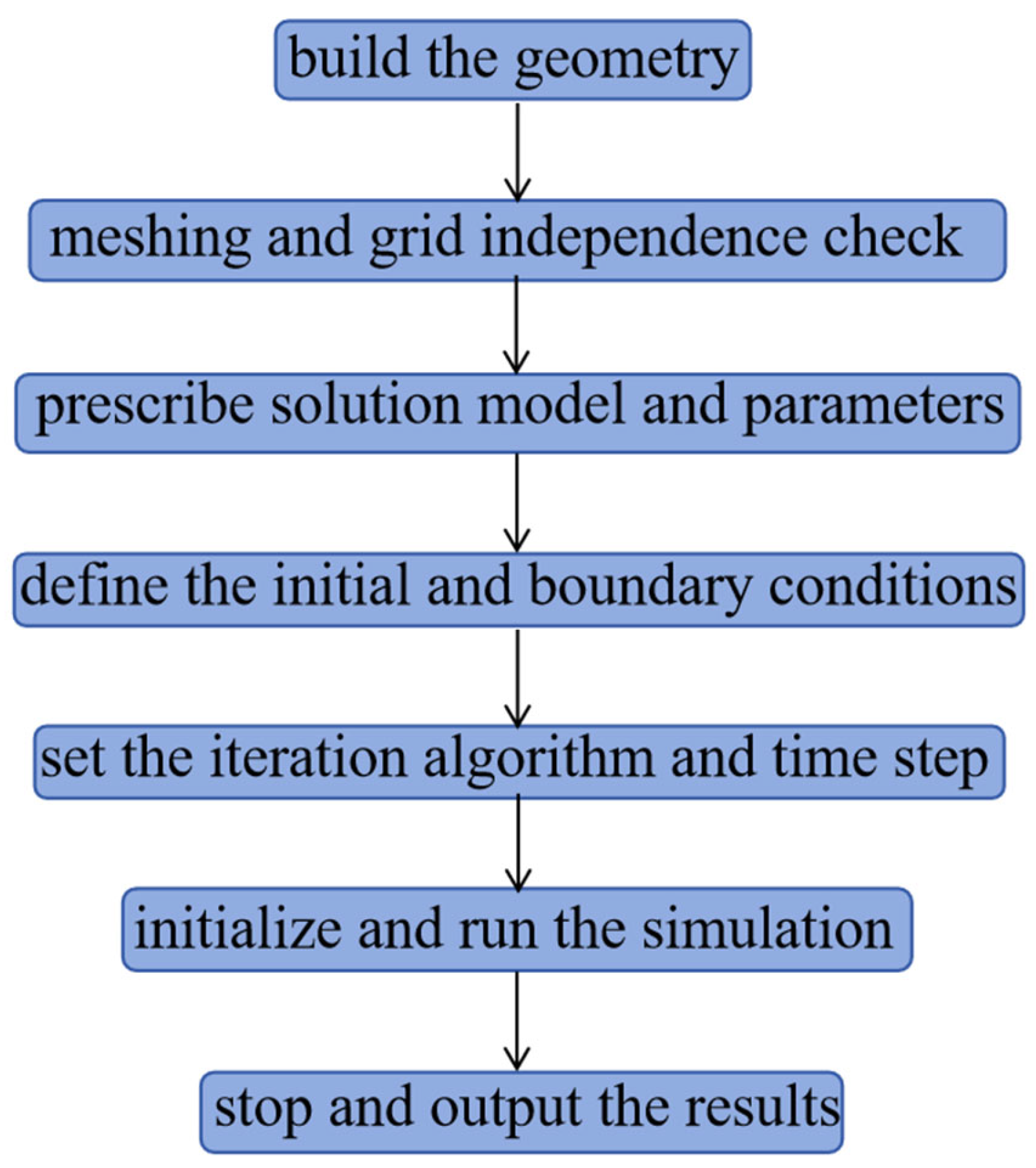
Figure 2.
Geometry configuration of the computational domain.
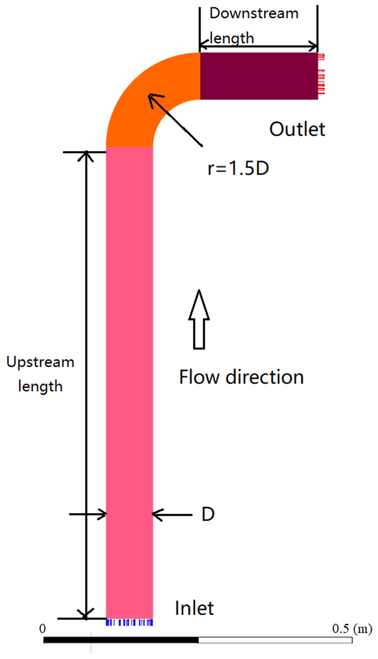
Figure 3.
Mesh configuration of the domain: (a) overview, (b) inlet section, (c) near wall, (d) outer wall).
Figure 3.
Mesh configuration of the domain: (a) overview, (b) inlet section, (c) near wall, (d) outer wall).
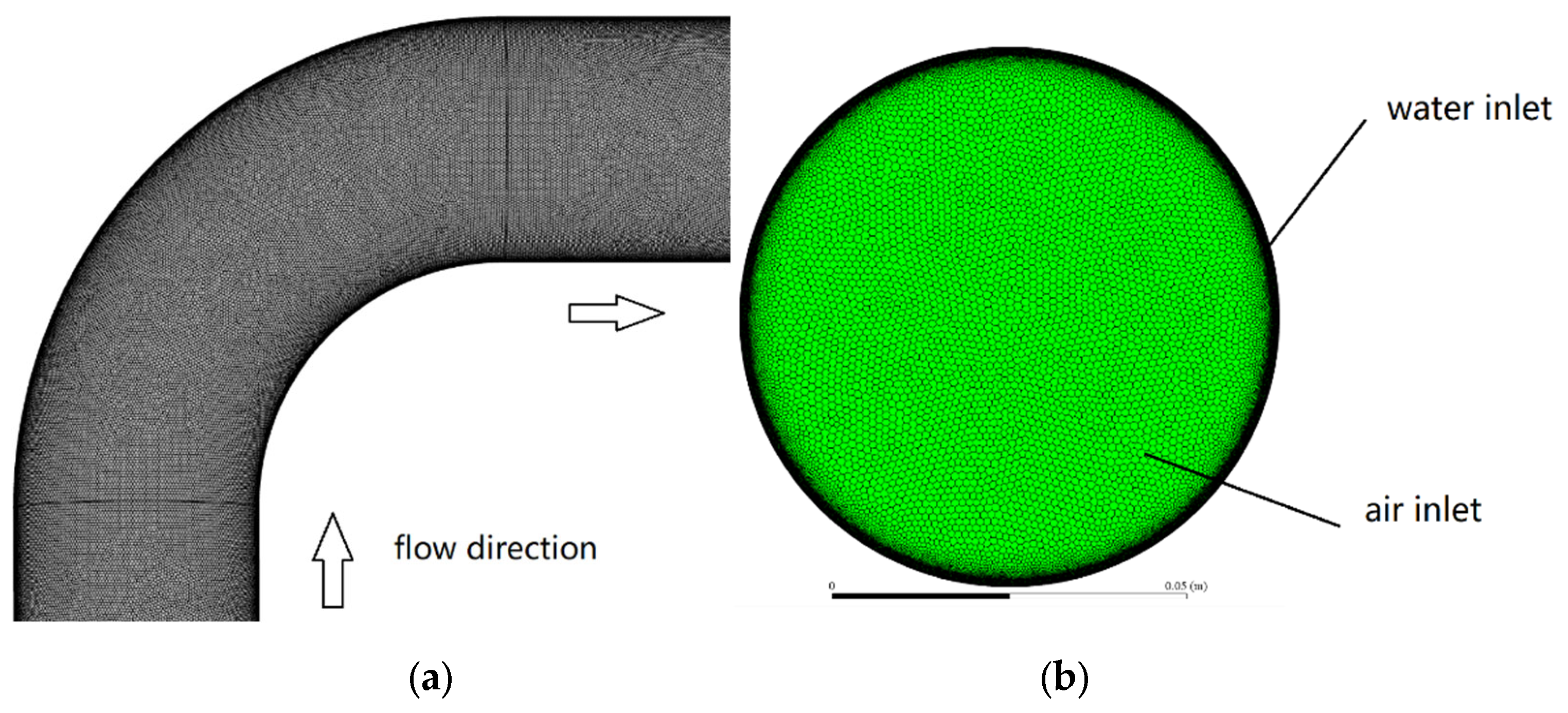
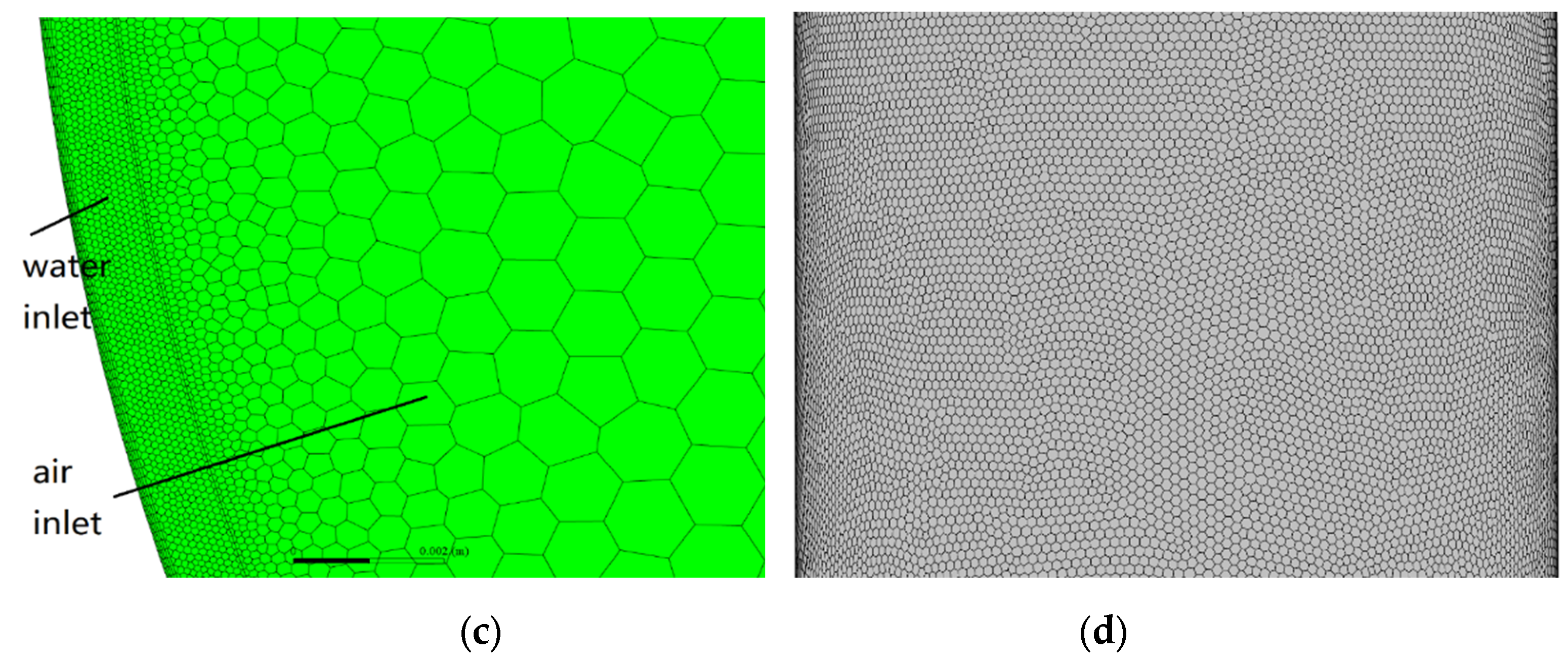
Figure 4.
Phase distribution and velocity vector of the pipeline: (a) overview; (b) enlarged view of the upstream; (c) enlarged view of elbow and downstream; (d) representative cross-sections.
Figure 4.
Phase distribution and velocity vector of the pipeline: (a) overview; (b) enlarged view of the upstream; (c) enlarged view of elbow and downstream; (d) representative cross-sections.
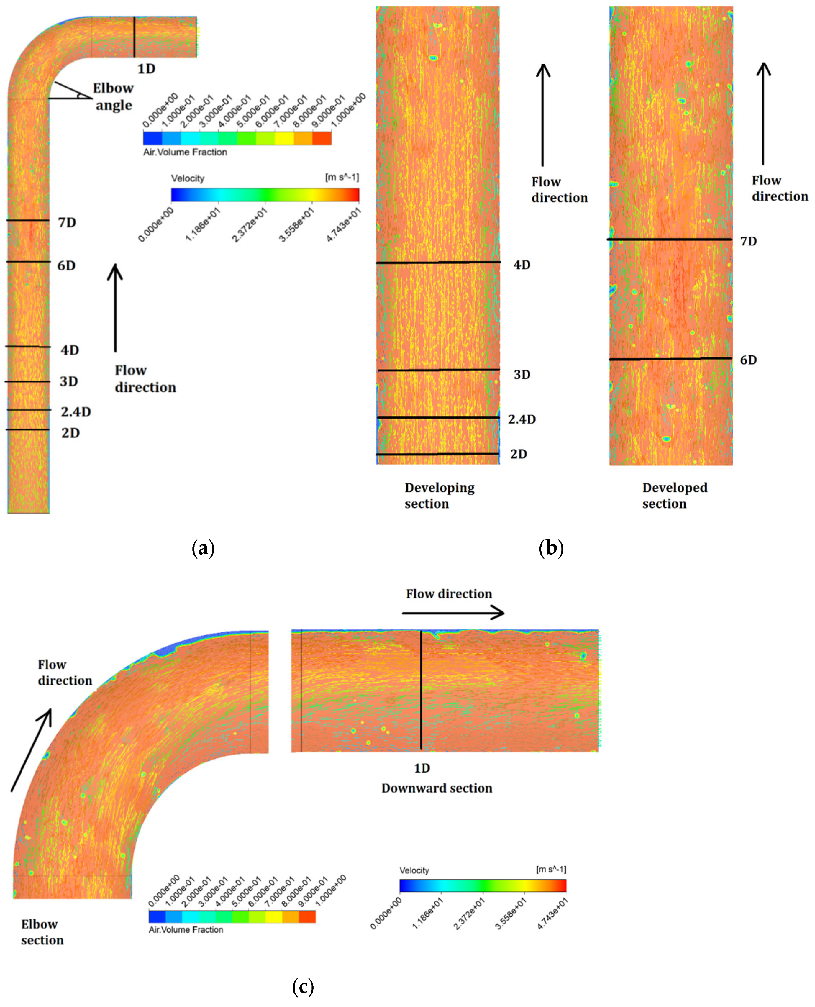
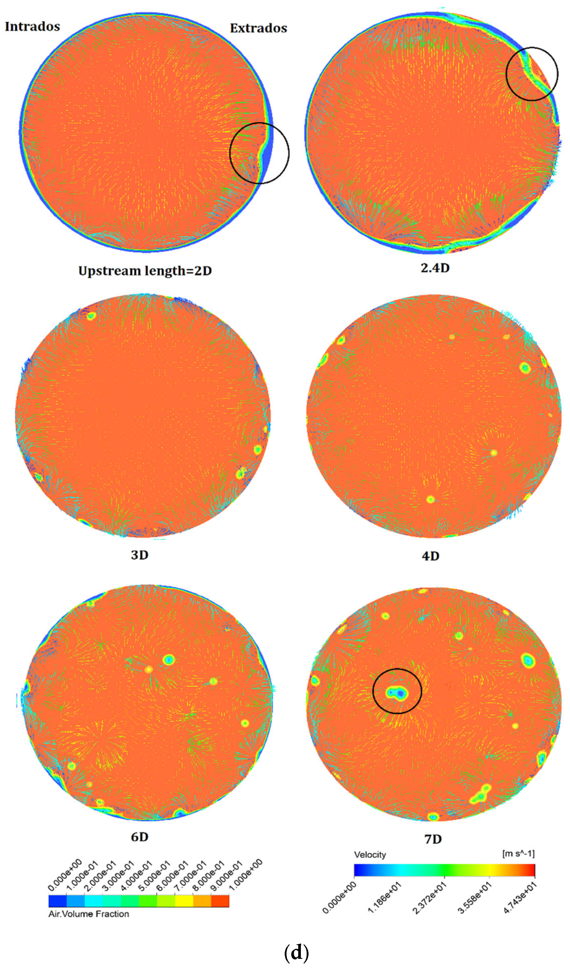
Figure 5.
Relationship between upstream length and area-weighted average void fraction of the pipe cross-sections.
Figure 5.
Relationship between upstream length and area-weighted average void fraction of the pipe cross-sections.

Figure 6.
Relationship between droplet diameter and droplet number distribution.
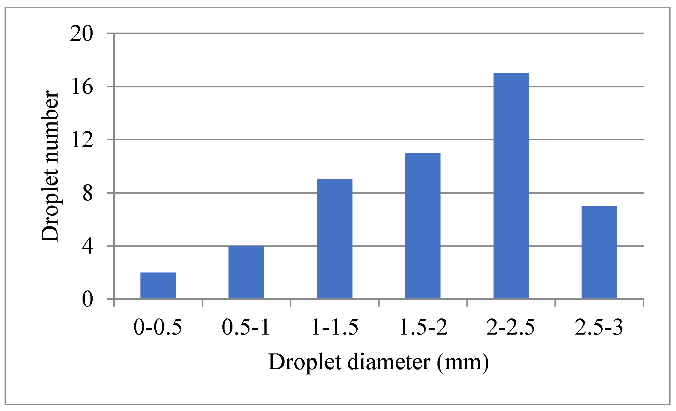
Figure 7.
Relationship between radial distance (from the wall) and droplet diameter.
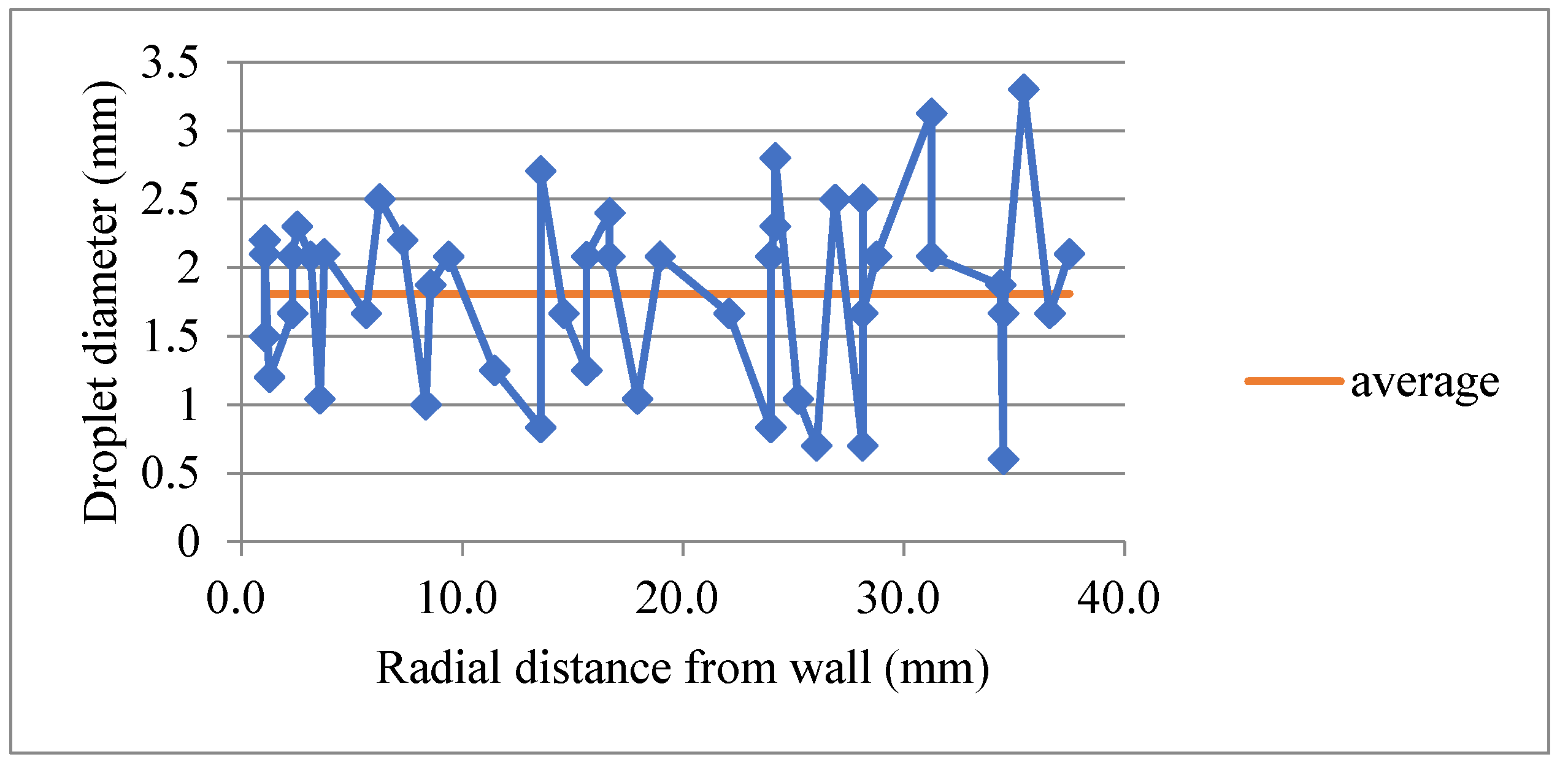
Figure 8.
Velocity distribution according to radial distance (from the wall).
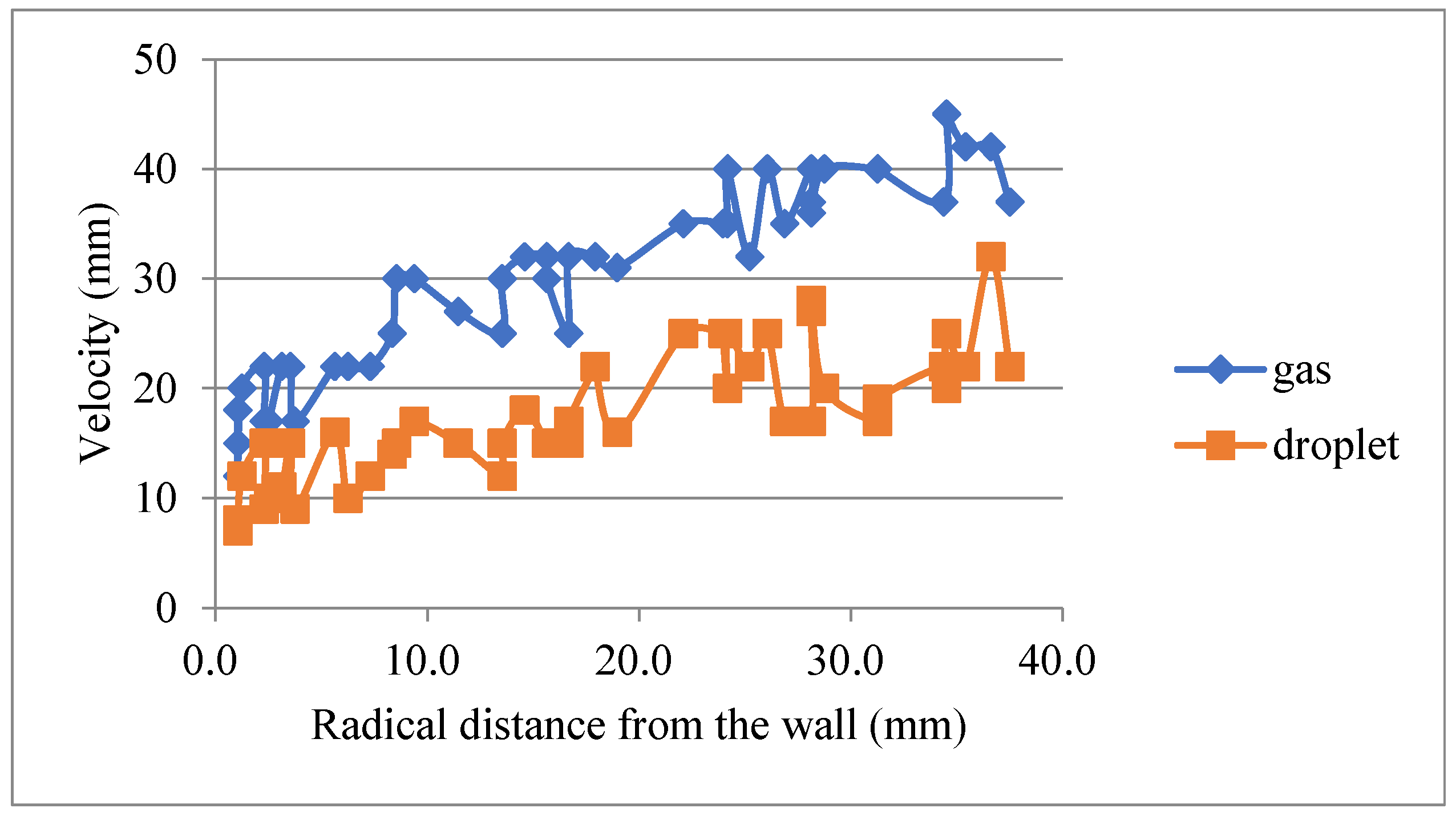
Figure 9.
Mechanism of the entrainment process in annular flow.

Figure 10.
Phases and velocity distribution for different elbow angles.


Table 1.
Literature review.
| Authors | Year | Summary of Work | Output |
|---|---|---|---|
| Wicks et al. [15] | 1960 | Isokinetic sampling experimental study on droplet entrainment characteristics | A model to calculate the droplet mass flow rate |
| Paleev et al. [16] | 1966 | Liquid film removal experimental study on entrainment characteristics | An empirical correlation to calculate film flow rate |
| Xu et al. [17] | 2013 | Water displacement characteristics investigation in inclined pipe | Critical value of oil flow rate to flush out trapped water |
| Haung et al. [18] | 2013 | Flow pattern observation in uphill and downhill pipes using high-speed camera | Experimental program to judge flow pattern in hilly-terrain flow |
| Parsi et al. [19] | 2015 | Experimental study on churn flow using wire-mesh sensor | Interfacial structures analysis of liquid film |
| Magnini et al. [20] | 2018 | Numerical study on effects of oil velocity and wall-wetting conditions on flow pattern | A model for predicting the drift velocity along upward pipes |
| Farokhipour et al. [21] | 2020 | Factors affecting elbow erosion and film distribution using simulation | Higher liquid velocity enhances film cushion and weakens erosion |
| Pshenin et al. [22] | 2022 | Hydrocarbon evaporation losses during loading of tanker fleets | A model of hydrocarbon vapor displacement from the inner part of a tanker |
| Korshak et al. [23] | 2023 | Water slug behavior and removal based on pumping liquid simulation | Slug removal algorithms that agree with experiment |
| Zhao et al. [24] | 2023 | Liquid distribution and erosion pattern of elbow under upward annular flow | Wave undercut and roll-wave entrainment mechanism |
Table 2.
Settings of the flow simulation.
| Items | Settings |
|---|---|
| Multiphase model | Volume of fluid |
| Turbulence model | k-e Realizable |
| Pressure–velocity coupling | SIMPLE |
| Interface modeling | Sharp |
| Spatial discretization | Second-order upwind |
| Primary phase | Air |
| Secondary phase | Water |
| Phase interaction | Surface tension force modeling |
| Surface tension coefficient | 0.072 N/m |
| Near-wall treatment | Enhanced wall treatment |
Table 3.
Boundary conditions of the flow simulation.
| Items | Settings |
|---|---|
| Air inlet (mass flow inlet) | 0.145 kg/s |
| Water inlet (mass flow inlet) | 0.456 kg/s |
| Outlet (pressure outlet) | Atmosphere |
| Turbulence intensity | 5% |
| Turbulence viscosity ratio | 10 |
| Wall | No slip |
| Wall contact angle | 90° |
Table 4.
Entrainment fraction obtained using different methods.
| Experimental Data | Oliemans’ Model | Ishii’s Model | CFD Data | ||
|---|---|---|---|---|---|
| 1520 | 2376 | 0.4 | 0.53 | 0.55 | 0.47 |
Table 5.
Variance distribution of droplet diameters.
| Radial Distance from Wall (mm) | Expectation (mm) | Variance |
|---|---|---|
| 0~10 | 1.85 | 0.19 |
| 10~20 | 1.76 | 0.36 |
| 20~30 | 1.76 | 0.51 |
| 30~40 | 1.86 | 0.63 |
Disclaimer/Publisher’s Note: The statements, opinions and data contained in all publications are solely those of the individual author(s) and contributor(s) and not of MDPI and/or the editor(s). MDPI and/or the editor(s) disclaim responsibility for any injury to people or property resulting from any ideas, methods, instructions or products referred to in the content. |
© 2024 by the authors. Licensee MDPI, Basel, Switzerland. This article is an open access article distributed under the terms and conditions of the Creative Commons Attribution (CC BY) license (https://creativecommons.org/licenses/by/4.0/).
Share and Cite
MDPI and ACS Style
Xie, Z.; Cao, X. Effect of Entrainment on the Liquid Film Behavior in Pipe Elbows. Energies 2024, 17, 1983. https://doi.org/10.3390/en17081983
AMA Style
Xie Z, Cao X. Effect of Entrainment on the Liquid Film Behavior in Pipe Elbows. Energies. 2024; 17(8):1983. https://doi.org/10.3390/en17081983
Chicago/Turabian StyleXie, Zhenqiang, and Xuewen Cao. 2024. "Effect of Entrainment on the Liquid Film Behavior in Pipe Elbows" Energies 17, no. 8: 1983. https://doi.org/10.3390/en17081983
Note that from the first issue of 2016, this journal uses article numbers instead of page numbers. See further details here.