Abstract
The two-phase countercurrent flow limitation (CCFL) in horizontal channels is important in relation to nuclear reactor safety. In this study, we aim to investigate the CCFL characteristics and the flow behaviors in horizontal circular pipes with small diameters. The effects of pipe diameter and the water head in the upper plenum on CCFL characteristics are experimentally studied. An image-processing technique and statistical treatments are implemented to analyze the horizontal countercurrent flow. The results show that the CCFL characteristics for the horizontal circular pipes with small diameters can be well correlated using the dimensionless parameters, which are based on adding fluid viscosity to the Wallis parameters. The CCFL characteristics are significantly affected by the pipe diameter and are slightly affected by the water head above the horizontal pipe. The gas–liquid interface fluctuates with certain periods, and flow pattern transitions happen in the horizontal air–water countercurrent flow. As the air flow rate increases, the occurrence location of the liquid slug appears to shift towards the water entrance. In addition, the further away from the water entrance, the lower the average of liquid holdup.
1. Introduction
In a gas–liquid two-phase flow, countercurrent flow limitation (CCFL) refers to a state in which the liquid flow is restricted by the countercurrent gas flow. The CCFL phenomenon is frequently encountered in practical applications like nuclear reactors, packed columns, heat pipes, etc. [1]. In the pressurizer liquid level measurement system of a nuclear power plant, there exists a horizontal section connected to the pressurizer. An orifice obstruction is installed in the horizontal pipe section. Steam and water flow countercurrently in the pipe section. However, CCFL may occur in the horizontal section in some cases. This could introduce inaccuracies in the measurement of the liquid level and affect the steady operation of the system [2]. In addition, CCFL may take place in the horizontal channel where steam and cold water flow in countercurrent when the emergency core coolant (ECC) water is supplied to the horizontal pipe during a loss of coolant accident (LOCA) or small break loss of coolant accident (SBLOCA). The occurrence of CCFL is closely related to nuclear reactor safety [3]. Besides the nuclear reactor, CCFL phenomena also exist in other practical industrial applications such as marine diesel engines, steam generation and refrigeration systems, oil and gas pipelines, etc. [4]. Therefore, it is necessary to study the CCFL phenomenon in horizontal countercurrent flow.
Table 1 lists published CCFL experiments in horizontal channels. It can be found in Table 1 that most research studies were carried out in rectangular channels. Because of the three-dimensional shape limitation of the interfacial structure in circular pipes, some investigators conducted experiments in rectangular channels in order to acquire better visual observation and optical quality [5]. However, circular pipes are commonly used in practical applications. The flow behaviors of the two-phase countercurrent flow in circular channels are different from those in rectangular channels. For example, corner vortices only appear in rectangular channels. The CCFL characteristics and the interfacial behaviors in rectangular channels also appear to be different from those in circular pipes.
Bankoff and Lee [6] stated that for large pipes (), the pipe diameter has no influence on the critical gas velocity, whereas the critical velocity is strongly affected by the diameter of small pipes [7,8]. It can be seen in Table 1 that there are few studies on horizontal countercurrent flow in relatively small-diameter pipes. Ma et al. [9] pointed out that the viscous force becomes more active in small pipes than in large pipes. The CCFL characteristics and the flow behaviors in small pipes appear to be different from those in large pipes. Therefore, more CCFL data and visual data for small-diameter pipes are needed to explore the CCFL characteristics and flow behaviors in horizontal countercurrent flow. Besides geometrical characteristics, fluid properties are also an important factor affecting CCFL [10,11,12].

Table 1.
CCFL experiments in horizontal channels.
Table 1.
CCFL experiments in horizontal channels.
| Authors | Test Fluid | Test Section | Conclusion |
|---|---|---|---|
| Wallis and Dobson (1973) [13] | Air–water | Rectangular channel: a = 0.0254, 0.089 m; b = 0.0254, 0.076–0.305 m | They presented a criterion for the occurrence of slug or plug flow in a horizontal rectangular channel. |
| Gardner (1983) [14] | Air–water | Circular pipe: D = 0.072 m | They developed a flooding criterion in horizontal countercurrent flow. |
| Bankoff et al. (1987) [15] | Steam–water | Rectangular channel: a = 0.095 m; b = 0.095 m | They developed a countercurrent flow regime map and explored the mechanism of hysteresis effects. |
| Ansari and Nariai (1989) [16] | Air–water | Rectangular channel: a = 0.05 m; b = 0.1 m | They observed three zones during slug initiation. They proposed that the short wavelength waves create slugs. |
| Wang and Kondo (1990) [3] | Air–water | Rectangular channel: a = 0.035 m; b = 0.02, 0.035, 0.05 m | They proposed an instability criterion including a viscous term. They observed various flow patterns under different void fractions. |
| Choi and No (1995) [17] | Air–water | Circular pipe: D = 0.04, 0.06, 0.07 m | They proposed two flooding mechanisms. They investigated the geometrical factors on flooding. |
| Chun et al. (2000) [18] | Steam–water, air–water | Circular pipe: D = 0.083 m | They studied the effect of steam condensation on CCFL. The gas flow rate required for the occurrence of CCFL for steam–water countercurrent flow is larger than that for air–water countercurrent flow. They found that the condensation effect on CCFL increases when the system pressure, the pipe diameter, or the subcooling is increased. |
| Gargallo (2005) [19] | Air–water | Rectangular channel: a = 0.11 m; b = 0.09 m | They observed hydraulic jump and flow reversal. They proposed that subcritical flow is necessary for the onset of flow reversal. |
| Wintterle et al. 2008 [20] | Air–water | Rectangular channel: a = 0.11 m; b = 0.09 m | They discussed the velocity fields, velocity fluctuations, and void fraction distributions in countercurrent supercritical flow. |
| Ma et al. (2020) [9] | Air–water | Circular pipe: D = 0.02, 0.04, 0.07, 0.1, 0.13 m | They studied the effect of diameter on CCFL characteristics and proposed an empirical correlation applied to small-diameter pipes. |
| Dhar et al. (2022) [21] | Air–water | Rectangular channel: a = 0.012 m; b = 0.05 m | They investigated the effect of hydraulic jump on flow regime transition. |
Accurate identifications of the flow patterns are important for studying the flow behaviors in a gas–liquid flow. Flow patterns can be identified by the statistical characteristics of pressure signals and void fractions. As an important data analysis tool, statistical treatment was used to analyze pressure signal data [22,23], void fraction data [24,25], liquid film thickness data [26], etc. Besides direct acquisition during the experiment, the void fraction data could be acquired from visual pictures by employing an image-processing technique [27,28,29,30]. The image-processing technique can help in detecting the gas–liquid interface and then void fraction or liquid holdup can be obtained through calculation.
In our previous work, we experimentally studied the CCFL phenomena in horizontal channels with obstructions [31]. To investigate the CCFL phenomenon in a horizontal pipe without obstruction and improve the understanding of the obstruction effect on CCFL, we carried out this work. This work aims to study the CCFL characteristics and the flow behaviors in horizontal circular pipes with small diameters. Visualization experiments were performed. In this study, we tested two circular pipes with different diameters and three water heads above the horizontal pipe. CCFL characteristic curves based on dimensionless parameters were obtained and compared with the literature. Typical flow behaviors under different flow rates were analyzed. An image-processing technique and statistical treatments were employed to analyze the horizontal countercurrent flow. The results of this study will help to develop an in-depth understanding of CCFL in horizontal countercurrent flow. In addition, the CCFL data from the experiment will contribute to the CCFL data bank.
2. Experimental Setup
The experimental equipment is mainly composed of an upper tank, a lower tank, a water storage tank, and a horizontal test section (Figure 1). Air and water are employed in the experiment. Air flows into the lower tank through the air supply line, which mainly consists of an air compressor, a pressure regulator, an air filter, two rotameters, and several regulation valves. After flowing to the lower tank, the air then passes to the test section and finally exhausts to the environment via the upper tank. Water is injected from the water storage tank to the upper tank through the water supply line, which is mainly composed of a water pump and a flowmeter. The injected water in the upper tank then flows to the lower tank through the horizontal test pipe. The air and water in the test section form a horizontal countercurrent flow during the CCFL experiments.
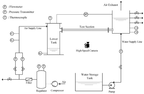
Figure 1.
Schematic of the experimental apparatus.
The horizontal test section is a circular acrylic pipe. In this study, two pipes with inner diameters of 0.019 and 0.029 m are tested, and the pipe lengths are 0.5 m. One end of the horizontal test pipe is connected to the upper tank, and the other end is lower tank. The height difference between the test pipe and the bottom of the upper tank is 0.05 m. The overflow bypass is set in the upper tank to keep a constant upper tank water level during an experiment. In this study, three different heights of the overflow bypass (0.2, 0.4, and 0.6 m) are arranged to explore the influence of the water head. The lower tank is a 0.21 m diameter and 1.0 m height cylindrical vessel. The lower tank water level is measured by a pressure transmitter installed in the bottom of the lower tank.
The experimental procedure is as follows: (a) Turn on the water pump to inject water into the upper tank. (b) Turn on the air compressor and regulate the air flow rate to a high value to ensure no falling water flows into the lower tank. (c) Switch on the overflow valve in the upper tank to obtain a constant upper tank water level. (d) Regulate the air flow rate to a specified value at which the water in the upper tank can flow to the lower tank. (e) Switch on the data acquisition instrument to collect the experimental data when the air–water flow achieves a quasi-steady condition. (f) Regulate the injected air at various flow rates to conduct other experimental cases. A duration of at least 5 min is carried out for each air flow rate case. In addition, repeated experiments are performed for each case.
In this experiment, the water flow rate that flows via the test pipe is calculated by the rise rate of the lower tank water level. The air flow rate is measured by two parallel rotameters with various instrument ranges. The ranges of the two rotameters are 0.09~0.90 m3/h and 0.8~8.0 m3/h, respectively. Besides the working fluid flow rates, temperature and pressure signals are also acquired in the experiment. The air temperature in the lower tank and the water temperature in the upper tank are measured by two T-type thermocouples. The pressure difference between the lower tank and the upper tank is measured by a Rosemount 3051CD pressure transmitter, of which the instrument range is 0~10 kPa. In the experiment, the inclination angle of the horizontal pipe is 0°, for which the uncertainty is ±0.05°. The measurement accuracies of the T-type thermocouples, the pressure transmitters, and the flowmeters are ±0.5 K, ±0.1%, and ±0.25%, respectively. All signal data are collected by a data acquisition instrument (Fluke 2680A). Moreover, a high-speed camera (Phantom V411) is employed to capture the visual image data of the horizontal countercurrent flow.
Table 2 shows the test matrix. Test sections with different diameter (D) values and various water heads above the horizontal pipe (H) are tested. The ranges of air superficial velocities () are 0.0929~0.5322 m/s for the 0.019 m diameter pipe and 0.1549~3.1490 m/s for the 0.029 m diameter pipe. The ranges of the water superficial velocity () values are 0.0040~0.0357 m/s for the 0.019 m diameter pipe and 0.0002~0.0706 m/s for the 0.029 m diameter pipe.
Table 2.
Test matrix of the experiments.
3. Results and Discussion
3.1. CCFL Characteristics
In this study, the obtained CCFL data characterize CCFL characteristics, which are different from the onset of CCFL [32]. In a countercurrent flow, the onset of CCFL is a critical state at which the gas flow starts to impede the liquid flow. Whereas the CCFL characteristics refer to the quasi-steady states where the liquid flow is impeded by the gas flow and the liquid does not fully flow out of the outlet. Figure 2 depicts the CCFL characteristics curves of the horizontal pipes with different diameters based on the Wallis correlation [33]. The Wallis correlation is in a linear relationship based on two dimensionless parameters and , i.e., the Wallis parameters. The Wallis parameters ( and ) are defined as follows:
where is the gas/liquid superficial velocity, is the gas/liquid density, is the acceleration of gravity, and D is the characteristic length. Based on the Wallis parameters, the Wallis correlation is defined as
where m and C are constants.
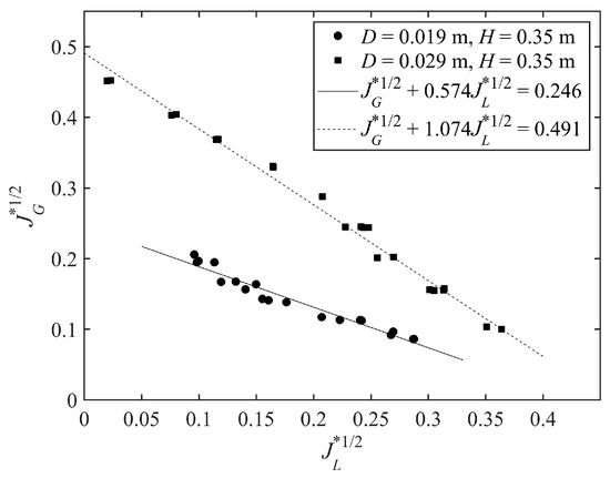
Figure 2.
Effect of pipe diameter on CCFL characteristics.
Figure 2 shows that the pipe diameter has great effects on CCFL. For a fixed gas superficial velocity, the flooding liquid velocity increases as the pipe diameter increases. Moreover, the ZLP point is higher for the larger diameter pipe.
For horizontal pipes with small diameters, Ma et al. [9] developed a new dimensionless parameter () to predict CCFL characteristics. considers the fluid viscosity effect and is defined as follows:
Based on , Ma et al. [9] fitted a linear correlation applied to horizontal flow in the diameter range of 0.02~0.1 m. The linear correlation is given below.
Figure 3 shows a comparison of the present CCFL data with the experimental results of Ma et al. [9]. The linear CCFL empirical correlation, i.e., Equation (5), is marked as the black solid line. The experimental CCFL data are well predicted by Equation (5). The relative errors between the experimental data and the predictions of Equation (5) are less than 12%.
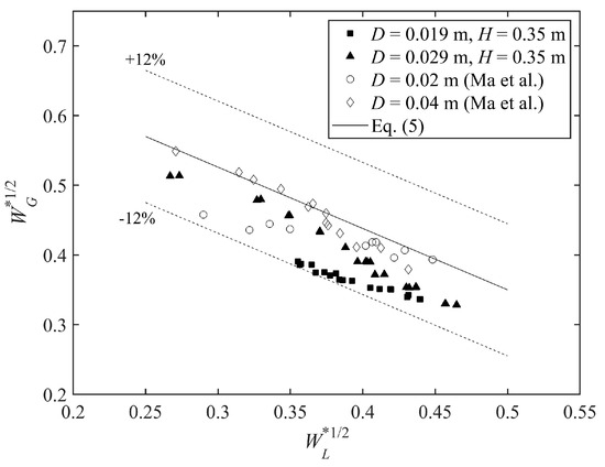
Figure 3.
CCFL data [9].
Besides geometrical parameters, the water head above the horizontal pipe is also an important factor in studies of CCFL characteristics. Ohnuki [34] stated that CCFL characteristics are not affected by the water head. Navarro [35] reported that CCFL characteristic curves for various water heads show no difference when the water head is below 0.04 m. When the water head is higher than 0.04 m, an increase in the water head results in a decrease in flooding gas velocity. The influence of the upper tank water head on CCFL characteristics is described in Figure 4. The diameters of the test pipes are 0.019 m. It can be found that the water head above the horizontal pipe slightly affects the CCFL characteristics. The flooding air velocity decreases as the water head increases. This result is in agreement with that of Navarro [35]. Yu et al. [36,37] also stated that the discrepancies in the CCFL data under various water levels are small but cannot be negligible.
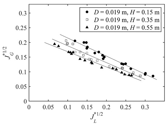
Figure 4.
Effect of the water head on CCFL characteristics.
3.2. Flow Behaviors
The test section with D = 0.019 m and H = 0.35 m was selected to carry out the visual observations and the signal analyses. The air–water flows in the horizontal pipe are not always stratified but in a quasi-steady state, where flow pattern transitions exist within certain periods. Figure 5, Figure 6 and Figure 7 show the flow behaviors of the horizontal countercurrent flow during CCFL at different flow rates.
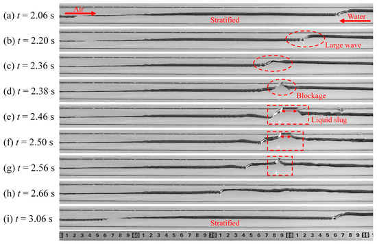
Figure 5.
Flow behavior at , .
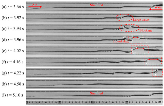
Figure 6.
Flow behavior at , .
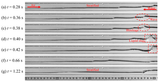
Figure 7.
Flow behavior at , .
Figure 5 shows the flow behavior in the test pipe within a flow cycle at , . Air and water are stratified at t = 2.06 s (Figure 5a). A large wave appears near the water entrance and then propagates to the left. Because the water flow rate in this case is high, the water level in the test section is high, and the crest of the wave almost reaches the upper pipe wall (Figure 5a–c). Therefore, the water in the pipe is more easily blown up to the upper pipe wall. The flooding air velocity is thus low in this case. After the wave moves a certain distance, the water wave is blown up by the air flow, and a liquid blockage forms at the location of the wave crest (Figure 5d). The liquid slug blocks the air from passing through the pipe, leading to the accumulation of air and an increase in the lower tank pressure. The incoming water gradually accumulates at the blockage, and the liquid slug occurs (Figure 5e). The occurrence of flow pattern transition from stratified flow to slug flow corresponds to the onset of liquid slug. This liquid slug initiated by the unstable wave development within the test pipe corresponds to the inner flooding [17]. The occurrence location of the liquid slug is further from the water outlet than the water entrance. Because the air flow rate in this case is relatively low, the air flow is not large enough to reverse the direction of the water flow. The liquid slug slightly shifts to the left, and the slug length gradually decreases until the slug disappears (Figure 5f,g). Then, the countercurrent flow transforms to a stratified state, and a flow cycle finishes (Figure 5h,i).
As the air flow rate increases (), the flow behavior in the test pipe during CCFL appears to change. As depicted in Figure 6, the flow pattern transition also takes place. Compared with Figure 5, the water level in Figure 6 is lower, and the occurrence location of the blockage slightly shifts to the water entrance (Figure 6c). The formation process of the liquid blockage is more severe accompanied by the droplet entrainment from the liquid blockage. A portion of water droplets is blown away. The liquid slug is then pushed forward to the water entrance by the flowing air [16]. In addition, the air-water interface fluctuation becomes more intense after the liquid slug takes place. With the development of the liquid slug, more and more incoming water accumulates at the slug, and the length becomes longer (Figure 6d–f). The air–water countercurrent flow reverts to stratified after the liquid slug flows into the upper tank (Figure 6h).
At , , the air flow rate continues to increase, and the water level in the horizontal pipe further decreases (Figure 7). The occurrence location of the blockage is closer to the water entrance. The maximum length of the slug is shorter than that in Figure 6. This is because the formation location of the liquid slug is very close to the water entrance, and the development distance for the liquid slug is short. In addition, the development velocity of the liquid slug towards the water entrance increases with the air velocity increasing.
3.3. Pressure Signal Analysis
The differential pressure between the upper tank and the lower tank (DP) was measured in the experiment. The acquired pressure signal can reflect the flow behaviors to some extent. Figure 8 depicts the fluctuations in DP over time during CCFL under different cases. It can be found that DP is not in constant pressure but fluctuates over time within a certain range.
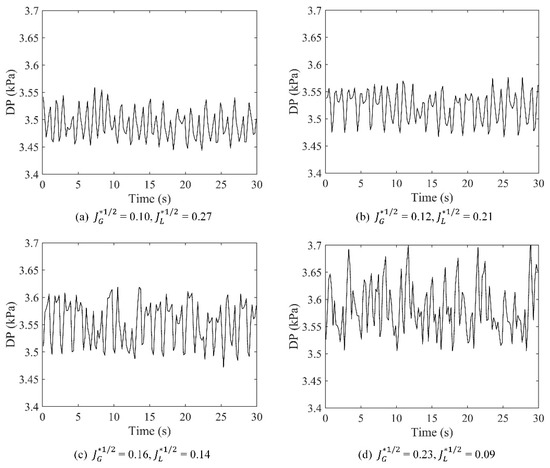
Figure 8.
Fluctuations in DP over time.
Figure 9 depicts the fluctuation in DP over time in one cycle at , . It can be seed that in one cycle, DP fluctuates within a certain range. A fluctuation cycle of DP includes a pressure decrease phase and a pressure increase phase. The decrease phase of DP corresponds to a stratified flow in the test section (Figure 5a–c), which indicates that the air in the lower tank can flow through the test pipe successfully. The minimum DP indicates the occurrence of the flow pattern transition from stratified flow to slug flow (Figure 5d). With the development of the slug, the value of DP increases over time (Figure 5d–g). This is because the air flow is blocked by the liquid slug from passing through the test pipe, resulting in the accumulation of air and an increase in lower tank pressure. When the slug disappears and the air–water flow reverts to stratified, the value of DP reaches its maximum (Figure 5h).
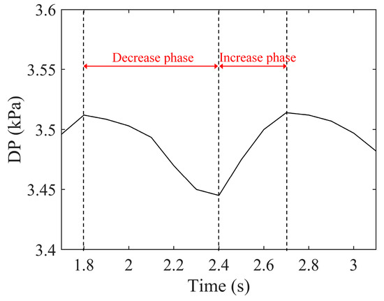
Figure 9.
Fluctuation in DP over time in one cycle at , .
The probability density function (PDF) is implemented to analyze the distribution of DP in the time domain. Figure 10 describes the PDFs of DP for different flow rates. The PDF curves are not essentially single-peaked, some of them are multi-peaked curves. At low air flow rates, the distribution ranges of DP are narrow, and the peak of the probability density is high, i.e., the distributions of the PDF curves are centralized. While the PDF curves are more dispersed with the air velocity increasing. Because the high air flow rate inducing high lower tank pressure, the DP distribution gradually shifts to higher pressures as the air velocity increases.
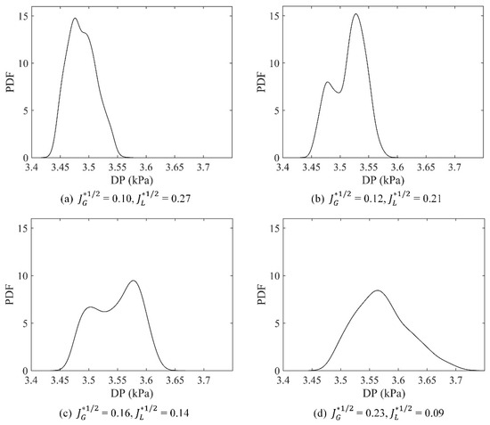
Figure 10.
PDFs of DP.
As mentioned above, the pressure signal DP fluctuates with a certain cycle. In order to analyze the pressure signal in the frequency domain and acquire the fluctuation cycle of DP, power spectral density (PSD) is implemented. Figure 11 depicts the PSD curves of the pressure signal DP at different fluid flow rates. The frequency band corresponding to the peak of PSD is named the dominant frequency, which is marked as a dotted line in the figure. As can be seen in Figure 11, the dominant frequencies of DP fluctuation for different flow rates are all around 1.0 Hz. Take Figure 11a as an example, the dominant frequency of the DP fluctuation is 1.0 Hz, which means the fluctuation cycle of DP is 1.0 s. As shown in Figure 5, the periodic flow pattern transitions occur in the horizontal countercurrent flow during CCFL. At , the period is about 1.0 s according to visual observation, which is equal to the fluctuation cycle of DP. This indicates that the pressure difference significantly affects the horizontal countercurrent flow, and the pressure signal can reflect the flow behaviors to some extent.
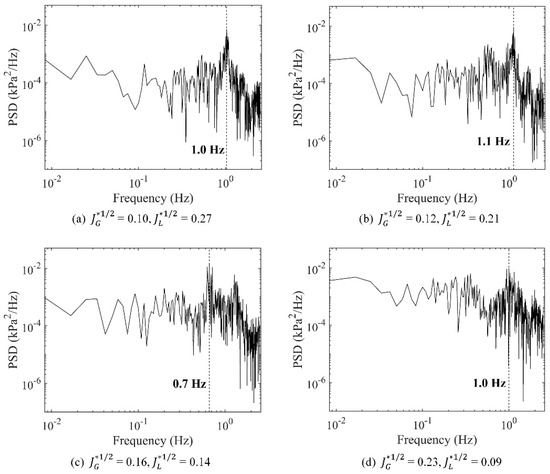
Figure 11.
PSDs of DP.
The variation in the statistical characterization of DP, including the average (Me) and the standard deviation (Sd) of DP is depicted in Figure 12. The average DP increases as the air velocity increases, and the increase rate gradually decreases (Figure 12a). Moreover, the standard deviation of DP also increases as the air velocity increases, indicating that the distributions of DP are more dispersed at high air velocities (Figure 12b).
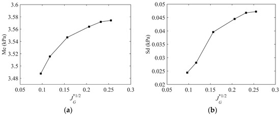
Figure 12.
Variation in the statistical characterization of DP with . (a) The average of DP; (b) The standard deviation of DP.
3.4. Liquid Holdup Data Analysis
The analyses of gas–liquid interface behaviors during CCFL are of significance in the studies of countercurrent flows. The gas–liquid interface can be quantified using image-processing techniques to acquire liquid holdup data in horizontal test pipes. The flow behaviors of the countercurrent flow in the test section were captured by a high-speed camera during the experiment. Based on captured video files, a MATLAB R2020a program was developed to detect the interface and calculate liquid holdup data. Accurate detection of the interface and pipe boundaries is the basis of calculating liquid holdup in a test pipe. For an original image extracted from the video, the image-processing procedure is as follows (Figure 13).
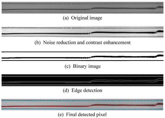
Figure 13.
Detection of pipe boundaries and the gas–liquid interface.
The first step is to reduce noise and enhance contrast (Figure 13b). Pipe boundaries and the gas–liquid interface can be easily distinguished from the air/water phase. Next, the processed image is binarized to determine the pixel threshold of the image (Figure 13c). Edge detection is then performed on the binary image. Because the pipe wall and interface have a certain thickness, two edge lines are detected for the pipe wall and interface (Figure 13d). To calculate the liquid holdup, the average pixels of the two edges of the interface are chosen as the final pixels of the gas–liquid interface, and the pixels of the inner pipe wall are chosen as the final pixels of the pipe boundaries. The final detected pixels of the gas–liquid interface and pipe boundaries are marked as a red dotted line and a cyan dotted line, respectively (Figure 13e). The liquid holdup in the test pipe with a circular cross-section is finally calculated by
where is the liquid holdup, is the pixel distance between the gas–liquid interface and the bottom of the pipe boundaries, and is the pixel distance of the pipe inner diameter.
A total sampling time of 12.0 s is adopted for liquid holdup data analysis in this study. Because the sampling rate of 500 fps for the high-speed camera is applied in the experiment, a total of 6000 frames is acquired for one case. To ensure efficiency, the images are chosen every 10 frames for liquid holdup analysis. In other words, the frequency of the liquid holdup data is 50 Hz in present study. The liquid holdup is not a constant value along the test pipe, so six measurement positions are arranged to analyze the liquid holdup at various locations (Figure 14). The distances between the water outlet of the pipe and the measurement positions (x) are 0.05, 0.13, 0.21, 0.29, 0.37, and 0.45 m.
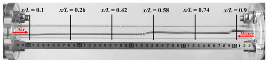
Figure 14.
Schematic diagram of the measurement positions.
The liquid holdup at x/L = 0.9, which is the measurement position closest to the water entrance, is analyzed. Figure 15 depicts the variations in liquid holdup with time at x/L = 0.9 under different cases. The liquid holdup fluctuates periodically in the time domain. The liquid holdup fluctuation corresponds to the periodic fluctuation in the gas–liquid interface. The peak of the liquid holdup reaches unity, which means the liquid phase fills the pipe cross-section at x/L = 0.9, i.e., the liquid slug takes place at this moment. In addition, the minimum of the liquid holdup decreases as the air velocity increases. In other words, the fluctuation ranges of the liquid holdup are larger at higher air velocities.
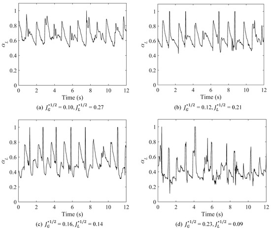
Figure 15.
Variation in liquid holdup with time at x/L = 0.9.
The PDF is also performed to further analyze the liquid holdup in the time domain. As shown in Figure 16, the PDFs are multi-peaked. The largest magnitudes of the peaks show a small discrepancy, but the liquid holdup corresponding to the peak of the PDF curve decreases as the air velocity increases. There exists a lower peak at the liquid holdup of 1, which means the occurrence of the liquid slug at x/L = 0.9. As the air velocity increases, the PDF curve spreads out along the x-axis with a wider range of the liquid holdup.
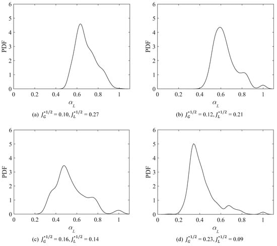
Figure 16.
PDFs of liquid holdup at x/L = 0.9.
The PSD of liquid holdup indicates the fluctuation characteristics of the gas–liquid interface. Figure 17 reveals the PSDs of liquid holdup at x/L = 0.9 for different flow rates. Take Figure 17a for example, the dominant frequency is 1.0 Hz. This means the interface fluctuation cycle is about 1.0 s, which is also the period of the slug occurrence. In addition, the dominant frequency of the liquid holdup fluctuation is equal to that of the DP fluctuation (Figure 11), indicating that the fluctuation cycle of DP is the same as the interface fluctuation cycle and the slug occurrence cycle.
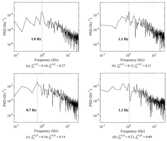
Figure 17.
PSDs of liquid holdup at x/L = 0.9.
Figure 18 describes the PDFs of liquid holdup at various measurement positions under and . As shown in the figure, the peak of the PDF curve tends to decrease when the position is away from the water outlet. In the left-side region (), the fluctuation ranges of liquid holdup are relatively small, and the liquid holdup values are low. On the one hand, because the water flows from the upper tank to the lower tank and the countercurrent flow in the test pipe is actually in subcritical conditions, the water level in the left-side region is lower than that in the right-side region. On the other hand, compared with the right-side region of the test pipe, the interface fluctuation in the left-side region is not that severe, and no liquid slug occurs in the left-side region.
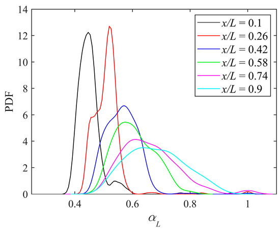
Figure 18.
PDFs of liquid holdup at various measurement positions under and .
Figure 19 shows the average and the standard deviation of liquid holdup under different cases. For a specified flow rate, the further away from the water entrance (x/L = 1), the lower the average liquid holdup (Figure 19a). The average increases as the air flow rate decreases. This is because more space in the pipe is occupied by the air at higher air flow rates, leading to the lower water level and liquid holdup. The standard deviation tends to increase with the distance from the water outlet (Figure 19b). This means the gas–liquid interface fluctuates more severely.
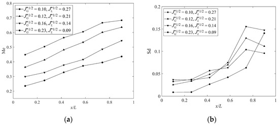
Figure 19.
The statistical characterization of liquid holdup at various measurement positions under different cases. (a) The average of liquid holdup; (b) The standard deviation of liquid holdup.
4. Conclusions
This paper carried out air–water CCFL experiments in horizontal circular pipes with small diameters. The CCFL characteristics and flow behaviors of the horizontal countercurrent flow were investigated. An image-processing technique and statistical treatments are applied to analyze the obtained data. The conclusions are as follows:
- (1)
- The CCFL characteristics for horizontal pipes with small diameters can be well correlated using the dimensionless parameter . The CCFL characteristics are significantly affected by pipe diameter and are slightly affected by the water head above the horizontal pipe. The flooding liquid velocity increases as the pipe diameter increases. The ZLP point is higher for larger-diameter pipes.
- (2)
- During the CCFL experiment, the gas–liquid interface fluctuates within certain periods, and flow pattern transitions happen in the horizontal countercurrent flow. As the air flow rate increases, the occurrence location of the liquid slug appears to shift towards the water entrance, and the formation process of the liquid blockage is more severe, accompanied by the droplet entrainment from the liquid blockage.
- (3)
- For different flow rates, the average liquid holdup increases as the air flow rate decreases. The further away from the water entrance, the lower the average of liquid holdup. In addition, the dominant frequencies of the pressure signal and the liquid holdup are the same at the same flow rate.
Author Contributions
Conceptualization, X.Z. and N.W.; methodology, X.Z. and C.X.; validation, C.X. and M.G.; formal analysis, X.Z. and M.G.; investigation, X.Z.; resources, C.X. and N.W.; data curation, M.G.; writing—original draft preparation, X.Z.; writing—review and editing, X.Z. and N.W.; visualization, X.Z., C.X. and M.G.; supervision, N.W.; project administration, N.W. All authors have read and agreed to the published version of the manuscript.
Funding
This research received no external funding.
Data Availability Statement
The original contributions presented in the study are included in the article, further inquiries can be directed to the corresponding author.
Conflicts of Interest
Authors Chende Xu and Mingzhou Gu was employed by the China Nuclear Power Engineering Co., Ltd. The remaining authors declare that the research was conducted in the absence of any commercial or financial relationships that could be construed as a potential conflict of interest.
Nomenclature
| General Symbols | |
| a | width, m |
| b | height, m |
| D | inner diameter of pipe, m |
| g | acceleration of gravity, |
| H | water head above the horizontal pipe, m |
| j | superficial velocity, |
| dimensionless superficial velocity | |
| L | pipe length, m |
| Me | average |
| P | pixel distance |
| Sd | standard deviation |
| Greek alphabet | |
| void fraction | |
| viscosity, | |
| density, | |
| Superscript | |
| * | dimensionless |
| Subscript | |
| d | inner diameter of pipe |
| G | gas |
| h | water level height |
| K | gas/liquid |
| L | liquid |
| Abbreviations | |
| CCFL | countercurrent flow limitation |
| ECC | emergency core coolant |
| LOCA | loss of coolant accident |
| probability density function | |
| PSD | power spectral density |
| SBLOCA | small break loss of coolant accident |
| ZLP | zero liquid penetration |
References
- Al Issa, S.; Macian, R. A Review of CCFL Phenomenon. Ann. Nucl. Energy 2011, 38, 1795–1819. [Google Scholar] [CrossRef]
- Zhao, D.; Xu, C.; Wang, Z.; Zhu, X.; Li, Y.; Chi, X.; Wang, N. Countercurrent Flow Limitation in a Pipeline with an Orifice. Energies 2023, 16, 222. [Google Scholar] [CrossRef]
- Wang, H.; Kondo, S. A Study on the Stratified Horizontal Counter-Current Two-Phase Flow. Nucl. Eng. Des. 1990, 121, 45–52. [Google Scholar] [CrossRef]
- de Sampaio, P.A.B.; Faccini, J.L.H.; Su, J. Modelling of Stratified Gas-Liquid Two-Phase Flow in Horizontal Circular Pipes. Int. J. Heat Mass Transf. 2008, 51, 2752–2761. [Google Scholar] [CrossRef]
- Deendarlianto; Vallée, C.; Lucas, D.; Beyer, M.; Pietruske, H.; Carl, H. Experimental Study on the Air/Water Counter-Current Flow Limitation in a Model of the Hot Leg of a Pressurized Water Reactor. Nucl. Eng. Des. 2008, 238, 3389–3402. [Google Scholar] [CrossRef]
- Bankoff, S.G.; Lee, S.C. A Critical Review of the Flooding Literature. Multiph. Sci. Technol. 1986, 2, 95–180. [Google Scholar] [CrossRef]
- Pushkina, O.L.; Sorokin, Y.L. Breakdown of Liquid Film Motion in Vertical Tubes. Heat Transf. Sov. Res. 1969, 1, 56–64. [Google Scholar]
- Wallis, G.B.; Makkenchery, S. The Hanging Film Phenomenon in Vertical Annular Two-Phase Flow. J. Fluids Eng. 1974, 96, 297–298. [Google Scholar] [CrossRef][Green Version]
- Ma, Y.; Shao, J.; Lyu, J.; Peng, J. Experimental Study on the Effect of Diameter on Gas–Liquid CCFL Characteristics of Horizontal Circular Pipes. Nucl. Eng. Des. 2020, 364, 110645. [Google Scholar] [CrossRef]
- Drosos, E.I.P.; Paras, S.V.; Karabelas, A.J. Counter-Current Gas-Liquid Flow in a Vertical Narrow Channel-Liquid Film Characteristics and Flooding Phenomena. Int. J. Multiph. Flow 2006, 32, 51–81. [Google Scholar] [CrossRef]
- Liu, Y.; Upchurch, E.R.; Ozbayoglu, E.M. Experimental Study of Single Taylor Bubble Rising in Stagnant and Downward Flowing Non-Newtonian Fluids in Inclined Pipes. Energies 2021, 14, 578. [Google Scholar] [CrossRef]
- Liu, Y.; Mitchell, T.; Upchurch, E.R.; Ozbayoglu, E.M.; Baldino, S. Investigation of Taylor Bubble Dynamics in Annular Conduits with Counter-Current Flow. Int. J. Multiph. Flow 2024, 170, 104626. [Google Scholar] [CrossRef]
- Wallis, G.B.; Dodson, J.E. The Onset of Slugging in Horizontal Stratified Air-Water Flow. Int. J. Multiph. Flow 1973, 1, 173–193. [Google Scholar] [CrossRef]
- Gardner, G.C. Flooded Countercurrent Two-Phase Flow in Horizontal Tubes and Channels. Int. J. Multiph. Flow 1983, 9, 367–382. [Google Scholar] [CrossRef]
- Bankoff, S.G.; Lee, S.C. Flooding and Hysteresis Effects in Nearly-Horizontal Countercurrent Stratified Steam-Water Flow. Int. J. Heat Mass Transf. 1987, 30, 581–588. [Google Scholar] [CrossRef]
- Ansari, M.R.; Nariai, H. Experimental Investigation on Wave Initiation and Slugging of Air-Water Stratified Flow in Horizontal Duct. J. Nucl. Sci. Technol. 1989, 26, 681–688. [Google Scholar] [CrossRef]
- Choi, K.Y.; No, H.C. Experimental Studies of Flooding in Nearly Horizontal Pipes. Int. J. Multiph. Flow 1995, 21, 419–436. [Google Scholar] [CrossRef]
- Chun, M.H.; Yu, S.O. Effect of Steam Condensation on Countercurrent Flow Limiting in Nearly Horizontal Two-Phase Flow. Nucl. Eng. Des. 2000, 196, 201–217. [Google Scholar] [CrossRef]
- Gargallo, M.; Schulenberg, T.; Meyer, L.; Laurien, E. Counter-Current Flow Limitations during Hot Leg Injection in Pressurized Water Reactors. Nucl. Eng. Des. 2005, 235, 785–804. [Google Scholar] [CrossRef]
- Wintterle, T.; Laurien, E.; Stäbler, T.; Meyer, L.; Schulenberg, T. Experimental and Numerical Investigation of Counter-Current Stratified Flows in Horizontal Channels. Nucl. Eng. Des. 2008, 238, 627–636. [Google Scholar] [CrossRef]
- Dhar, M.; Ray, S.; Das, G.; Kumar Das, P. Hydraulic Jump Induced Flooding and Slugging in Stratified Gas-Liquid Flow—An Experimental Appraisal. Exp. Therm. Fluid Sci. 2022, 134, 110617. [Google Scholar] [CrossRef]
- Catrawedarma, I.G.N.B.; Deendarlianto; Indarto. Statistical Characterization of Flow Structure of Air–Water Two-Phase Flow in Airlift Pump–Bubble Generator System. Int. J. Multiph. Flow 2021, 138, 103596. [Google Scholar] [CrossRef]
- Wijayanta, S.; Indarto; Deendarlianto; Catrawedarma, I.G.N.B.; Hudaya, A.Z. Statistical Characterization of the Interfacial Behavior of the Sub-Regimes in Gas-Liquid Stratified Two-Phase Flow in a Horizontal Pipe. Flow Meas. Instrum. 2022, 83, 102107. [Google Scholar] [CrossRef]
- Fossa, M.; Guglielmini, G.; Marchitto, A. Two-Phase Flow Structure Close to Orifice Contractions during Horizontal Intermittent Flows. Int. Commun. Heat Mass Transf. 2006, 33, 698–708. [Google Scholar] [CrossRef]
- Rodrigues, R.L.P.; Cozin, C.; Naidek, B.P.; Marcelino Neto, M.A.; da Silva, M.J.; Morales, R.E.M. Statistical Features of the Flow Evolution in Horizontal Liquid-Gas Slug Flow. Exp. Therm. Fluid Sci. 2020, 119, 110203. [Google Scholar] [CrossRef]
- dos Reis, E.; Goldstein Leonardo, J. Characterization of Slug Flows in Horizontal Piping by Signal Analysis from a Capacitive Probe. Flow Meas. Instrum. 2010, 21, 347–355. [Google Scholar] [CrossRef]
- Montoya, G.A.; Deendarlianto; Lucas, D.; Höhne, T.; Vallée, C. Image-Processing-Based Study of the Interfacial Behavior of the Countercurrent Gas-Liquid Two-Phase Flow in a Hot Leg of a PWR. Sci. Technol. Nucl. Install. 2012, 2012, 209542. [Google Scholar] [CrossRef][Green Version]
- do Amaral, C.E.F.; Alves, R.F.; Da Silva, M.J.; Arruda, L.V.R.; Dorini, L.; Morales, R.E.M.; Pipa, D.R. Image Processing Techniques for High-Speed Videometry in Horizontal Two-Phase Slug Flows. Flow Meas. Instrum. 2013, 33, 257–264. [Google Scholar] [CrossRef]
- Badarudin, A.; Setyawan, A.; Dinaryanto, O.; Widyatama, A.; Indarto; Deendarlianto. Interfacial Behavior of the Air-Water Counter-Current Two-Phase Flow in a 1/30 Scale-down of Pressurized Water Reactor (PWR) Hot Leg. Ann. Nucl. Energy 2018, 116, 376–387. [Google Scholar] [CrossRef]
- Hudaya, A.Z.; Widyatama, A.; Dinaryanto, O.; Juwana, W.E.; Indarto; Deendarlianto. The Liquid Wave Characteristics during the Transportation of Air-Water Stratified Co-Current Two-Phase Flow in a Horizontal Pipe. Exp. Therm. Fluid Sci. 2019, 103, 304–317. [Google Scholar] [CrossRef]
- Zhu, X.; Xu, C.; Gu, M.; Tang, S.; Wang, N. Experimental Study on Air-Water Countercurrent Flow Limitation in Horizontal Pipes with Different Types of Obstructions. Prog. Nucl. Energy 2024, 169, 105087. [Google Scholar] [CrossRef]
- Deendarlianto; Höhne, T.; Lucas, D.; Vierow, K. Gas-Liquid Countercurrent Two-Phase Flow in a PWR Hot Leg: A Comprehensive Research Review. Nucl. Eng. Des. 2012, 243, 214–233. [Google Scholar] [CrossRef]
- Wallis, G.B. Flooding Velocities for Air and Water in Vertical Tubes; Atomic Energy Establishment: Harwell, UK, 1961.
- Ohnuki, A. Experimental Study of Counter-Current Two-Phase Flow in Horizontal Tube Connected to Inclined Riser. J. Nucl. Sci. Technol. 1986, 23, 219–232. [Google Scholar] [CrossRef][Green Version]
- Navarro, M.A. Study of Countercurrent Flow Limitation in a Horizontal Pipe Connected to an Inclined One. Nucl. Eng. Des. 2005, 235, 1139–1148. [Google Scholar] [CrossRef]
- Yu, J.; Zhang, D.; Shi, L.; Wang, Z.; Yan, S.; Dong, B.; Tian, W.; Su, G.H.; Qiu, S. Experimental Investigation of Air-Water CCFL in the Pressurizer Surge Line of AP1000. Nucl. Technol. 2016, 196, 614–640. [Google Scholar] [CrossRef]
- Yu, J.; Zhang, D.; Shi, L.; Wang, Z.; Tian, W.; Su, G.H.; Qiu, S.Z. Experimental Research on the Characteristics of Steam-Water Counter-Current Flow in the Pressurizer Surge Line Assembly. Exp. Therm. Fluid Sci. 2018, 96, 180–191. [Google Scholar] [CrossRef]


Disclaimer/Publisher’s Note: The statements, opinions and data contained in all publications are solely those of the individual author(s) and contributor(s) and not of MDPI and/or the editor(s). MDPI and/or the editor(s) disclaim responsibility for any injury to people or property resulting from any ideas, methods, instructions or products referred to in the content. |
© 2024 by the authors. Licensee MDPI, Basel, Switzerland. This article is an open access article distributed under the terms and conditions of the Creative Commons Attribution (CC BY) license (https://creativecommons.org/licenses/by/4.0/).