Numerical Simulation of Fracturing Fluid Storage in Shale Reservoirs Based on Experimental Measurements of Stress Sensitivity of Hydraulic Fracture Network Conductivity

Abstract

Hydraulic fracturing is used in shale reservoir production, with low flowback rates and a large amount of fracturing fluid retained inside the reservoir. In this study, a stress sensitivity analysis experiment on the fracture inflow capacity was implemented to investigate the relationship between the hydraulic fracture (HF) and natural fracture (NF) inflow capacities and effective stress. A three-dimensional shale reservoir model was also constructed to couple the experimentally obtained laws with the numerical model to investigate the effects of the connection and closure of the fracture network on the retention of the fracturing fluid. The results show that the stress sensitivity of natural fractures is two orders of magnitude higher than that of hydraulic fractures. The seepage-absorption effect of capillary forces is not the whole reason for the large amount of fracturing fluid retention. The closure of the fracture network formed by natural and hydraulic fractures during the production process led to the storage of a large amount of fracturing fluid, and this process maintained the stability of the water production rate during the steady water production period.

1. Background

There has been an exponential increase in global energy consumption in the last several decades. According to the U.S. Energy Information Administration’s (EIA) latest Short-Term Energy Outlook (STEO) [1], consumption will reach 101.56 million barrels per day (mb/d) in the first quarter of 2024, with 101.77 mb/d in the second quarter and 102.85 mb/d in the third and fourth quarters. The data suggested that total demand in 2022 would be 99.36 mb/d. With the depletion of conventional energy sources, the share of non-conventional energy consumption has gradually increased in recent years. According to the U.S. Energy Information Administration (EIA) [2], the contribution of shale oil to the U.S. total oil consumption rose from only 12% in 2008 to more than 75% in 2022.

Due to the low porosity and low permeability of shale reservoirs, horizontal wells and multi-stage hydraulic fracturing techniques are employed during production, and a large amount of high-pressure fracturing fluid is injected into the reservoir for the stimulation and extension of fractures during development. A portion of the fracturing fluid is returned to the surface, while another portion is retained in the reservoir for a long period of time. In general, shale reservoirs have lower flowback rates than conventional reservoirs, but the rate varies greatly from shale reservoir to shale reservoir, ranging from as low as 5% in Haynesville to 50% in some areas of Barnett and Marcellus. To date, the reasons for the differences in the fracturing fluid flowback rate in different reservoirs are not clear, and the transport law of stagnant fracturing fluid within the reservoir and its impact on subsequent development are not fully understood.

Previous studies have shown that [3] the spontaneous seepage of fracturing fluid into the matrix near the fracture and its retention within the fracture system are the main reasons for the low flowback rate after fracturing. Holditch [4] investigated the capillary forces and relative permeability of the matrix near the fracture during hydraulic fracturing in tight gas reservoirs. The results show that higher capillary forces result in higher relative permeability of the water phase and the retention of the fracturing fluid, making it difficult for the fracturing fluid to return to the surface. Ehlig-Economides et al. [5] considered the morphology of the fracture network formed after fracturing and concluded that only 5% to 10% of the fracturing fluid lay in the propped fracture after fracturing. There are two modes of fracturing fluid retention within the reservoir: 1. un-propped areas in hydraulic fractures; 2. open natural fractures.

McClure [6] proposed that the complex fracture network formed after fracturing closed in a very short period of time. The fracturing fluid inside the fracture network is returned to the surface in less time than the closure time, resulting in a large amount of fracturing fluid being retained in the reservoir. Sharma et al. [7] listed five points of evidence for the presence of un-propped fractures that form in the complex fracture network after fracturing and continuously close during production. To conclude, some studies of fracturing fluid retention within the reservoir have been conducted and can confirm the presence of un-propped fractures in the fracture network formed at the end of fracturing. However, the contribution of this fracture to the fracture fluid return phase and retention has not been fully revealed. Zhao et al. [8] developed a numerical model to study the fracture network’s evolution during the nitrogen fracturing of shale reservoirs and found that tensile damage was considered the main cause of fracture formation and expansion. Nuclear magnetic resonance and 2.5-dimensional matrix–fracture visualization microfluidic models were used by Wu et al. [9] to investigate the effect of generated fractures on the fracturing fluid flowback rate. The unconnected secondary fractures increased the drainage area and decreased the fracturing fluid return rate. However, the connected secondary fracture is conducive to flowback. Liu and Christine [10] propose a numerical model for simulating pumping, well shut-in, choked flowback, and rebound when the well is shut in again through DFIT-return testing. The results showed that the injected fluid recovery was very low, indicating that the fluid remained in the primary and secondary fractures opened during the fracture injection process. Zhou et al. [11], through imbibition and flowback experiments on shale with variable fracture widths and NMR testing, found that the main state of a retained fracturing fluid is a liquid bridge, continuous water film, or patchy water film. They suggested adding drainage aids to reduce the amount of retained fracturing fluid during fracturing and to prolong the duration of the dominant gas seepage channel and the pure liquid phase seepage time by increasing the differential pressure during the production process.

Previous studies concluded that there are two mechanisms for fracturing fluid retention in the reservoir: 1. the retention of fracturing fluid in the formation causes a water-lock effect that reduces oil and gas conductivity and harms oil and gas production; 2. the retained fracturing fluid displaces a portion of oil from the matrix under the action of the huge capillary forces in shale reservoirs. Dehghanpour et al. [12] conducted shale core experiments showing that retained fracturing fluid damaged the reservoir and reduced conductivity. However, the water trapped in the reservoir induced the generation of new microfractures, which, in turn, increased production. Meng et al. [13] tested the spontaneous seepage process of shale by the nuclear magnetic resonance (NMR) technique and found that the obtained T2 spectrum of shale had a double-peak feature, but the double-peak increase during the spontaneous percolation process was asymmetric, indicating that the percolation process may have induced the generation of new microfractures. Nur and Sheng [14] suggested that in stress-sensitive or water-locked severe reservoirs, steady production at constant production rates for a long period of time may improve the ultimate recovery. In contrast, shut-in does not improve the ultimate recovery but can weaken the effect of water lock to a certain extent, and a constant production rate is significantly beneficial in improving the ultimate recovery in strongly permeable shale reservoirs. Lin et al. [15] found that the flowback is inversely proportional to the clay content of the shale through a combination of experiments and numerical simulations. High-salinity fracturing fluids or surfactant solutions can increase the flowback ratio. In addition, the injection pressure is directly proportional to the flowback, while matrix permeability is inversely proportional to the flowback. Niu et al. [16] developed a new model of the relative permeability of oil and water phases during rejection in shale formations based on a fractal approach. Shao et al. [17] found that the mineralization of the flowback fracturing fluid was much higher than that of the fracturing fluid by analyzing the change in mineralization before and after the flowback of the fracturing fluid. A high-salinity flowback fracturing fluid will produce salt crystallization in the late flowback and production stages, blocking fractures and pores and reducing the gas seepage capacity. Zhao et al. [18] conducted a series of indoor experiments and found that the lack of mesopores in the shale and the relatively weak heterogeneity between the layers make it more likely that a particular thickness of continuously developed shale will be the interlayer that delineates the superimposed gas-bearing system.

In general, the current research on fracturing fluids mainly focuses on the location of fracturing fluid storage, the storage mechanism, and the impact on subsequent development. The coupling between experimental data and numerical simulation has not been sufficiently studied. In this paper, we investigate the fracturing fluid storage law from a combination of experimental measurements and numerical simulations.

2. Experimental

2.1. Materials

A total of 10 natural outcropping cores from Gimsar were selected for this experiment. And the Brazilian splitting method was applied to all of them, in which columnar cores were put into a fracturing machine with their laying direction parallel to the cutting edge, thus forming artificial cracks in the cores. The fracture surface was sanded sequentially with 60-grit, 150-grit, and 320-grit sandpaper to ensure an initial roughness of approximately 2 mm. Afterward, they were divided into two groups, one of which was filled with sand to characterize the hydraulic fractures formed during hydraulic fracturing. Another group of cores was not filled with sand and was used to characterize natural fractures that were propped open during the fracturing process. The two groups of cores were saturated with kerosene at room temperature (25 °C) for 24 h. Figure 1 shows a core with fracture filled with sand.

2.2. Methods

In the process of numerical simulation, the determination of the fracture conductivity is more important than the determination of its permeability. Fracture conductivity is used to characterize the ability of hydrocarbons to flow inside the fracture system and is numerically equal to the product of the width of the fracture and the permeability of the fracture. However, in the case of fractures, the width is often not uniform, the surface of the fracture is not smooth, and the degree of roughness varies from place to place, so it is difficult to determine the width of the fracture at each place. It is difficult to obtain an accurate value for the conductivity of a fracture.

In the study described in this paper, our attention is focused on the change rule of the flow conductivity of fractures with the process of the reduction in closure stress. As the main flow channel, the contribution of fractures to the flow is much higher than that of the matrix. We focus on the degree of variability in fracture conductivity. Therefore, in this study, the permeability of the core matrix was not accurately measured. The changes in width, permeability, roughness, etc., caused by changes in effective stress near fractures can significantly affect the conductivity of fractures, and these series of changes are difficult to measure and consider. Wu et al. [19] proposed a method for characterizing the changing patterns of fracture conductivity:

$$\frac{\Delta p}{q}=\frac{\beta \rho L}{{(Dw)}^2}q+\frac{\mu L}{\left(k_{f}w\right)D}$$

where Δp is the pressure drop, MPa; q is the volumetric velocity, cm³/s; β is the Forchheimer coefficient, 1/cm; ρ is the fluid density, g/cm³; L is the length of the core, cm; D is the diameter of the core or fracture height, cm; w is the fracture width, cm; μ is the fluid viscosity, cp; and k_f is the fracture permeability, darcies. To calculate the fracture conductivity, $\frac{\Delta p}{q}$ was plotted against q; the fracture conductivity k_fw can then be calculated from the intercept without knowing β. The conductivity obtained after each pressure drop change is compared with the initial condition to obtain the normalized conductivity change curve.

2.3. Experimental Procedure

In the subsequent numerical simulations, the maximum pressure drop of the model was 26 MPa; in other words, in the course of the experiments, we had to consider the experimental condition where the maximum closure stress is 26 MPa. Considering the irreversible nature of core damage, the procedure of gradually increasing the perimeter pressure was selected for testing in the experiment. And the maximum pressure-bearing capacity of the gripper was 32 MPa, the initial confining pressure of the gripper was controlled at 4 MPa, and the downstream pressure was finally controlled at 4 MPa. The experimental procedure is specified as follows:

• We put the core into the gripper and confined the oil. One end of the core gripper was connected to N₂, the pressure at the outlet end was controlled to always be constant at 4 MPa, and the pressure at the inlet end was measured. The flow rate of N₂ (q) and the pressure difference (Δp) between the inlet and outlet ends were measured under these conditions. Figure 2 illustrates the core gripper used during the experiment.
• The flow rate of N₂ at the inlet end was varied, and the pressure difference between the inlet and outlet ends was measured for four sets of other N₂ flow rates, as well as the flow rate in that case.
• The relationship between $\frac{\Delta p}{q}$ and $q$ was plotted.
• The enclosure pressure was increased to 8 MPa, 12 MPa, 16 MPa, 20 MPa, 24 MPa, 28 MPa, and 30 MPa. The N₂ flow rate was controlled, the stabilized pressure drop was measured, and the experiment was repeated. After that, the relationship between the conductivity and the closure stress of the fractures in this core was obtained.
• By repeating the above experiments for the cores of Group 1 and Group 2, the relationship between fracture conductivity and closure stress was obtained.

3. Simulation

3.1. Model Setup

Numerical reservoir simulation techniques are now widely used to investigate the transport patterns of fracturing fluids inside reservoirs. In this study, a 3D reservoir numerical model was established with reference to field data from a Jimsar fracturing platform, and CMG (2021) [20] was used as a numerical simulator. The parameters of the field construction are shown in

Table 1. Construction data from a fracturing platform in Jimsar.

Parameters	Values
Horizontal segment length	1800 m
Number of clusters in single segment	8
Single-segment length	45 m
Fracturing fluid volume	72,000 m3
Target layer depth	3000 m
Target layer thickness	5 m

. Microseismic monitoring showed that a complex seam network was formed by natural fractures and hydraulic fractures after the hydraulic fracturing of the target layer. Three flow systems are considered in the model: matrix–matrix, matrix–fracture, and fracture–fracture.

Model assumption:

It is assumed that the hydraulic fracture expands in a plane perpendicular to the direction of the minimum horizontal principal stress and appears as a biplane plane crack. In this study, only a cluster of cracks was simulated for the simplicity of calculation, and inter-seam interference between cracks was not considered. The fracture pattern is symmetrical and uniformly distributed. The effect of gravity on the fluid’s transport in the horizontal direction is ignored, and the model properties change significantly in the near-fracture region. The whole reservoir can be seen as a strong water-wet reservoir, and the basic parameters of the model are shown in

Table 2. Basic model parameters.

Parameters	Values
Model grid	9 × 41 × 1
Model size (m)	200 × 6.5 × 5
Initial pressure (MPa)	40
Rock compressibility (KPa−1)	1 × 10−5
Matrix porosity (%)	0.1
HF porosity (%)	0.068
NF porosity (%)	0.03
Matrix permeability (mD)	0.01
HF conductivity (D·cm)	45
Initial matrix water saturation	0
Matrix HF water saturation	1
Matrix NF water saturation	1

.

Simulation procedure:

• After hydraulic fracturing construction, it is assumed that the amount of fracturing fluid is consistent for each fracture cluster and that the fracturing fluid completely props HFs and NFs. According to calculations, the total fracturing volume in each cluster of fractures is about 225 m³, the initial hydraulic fractures of the model contain 10% of the fracturing fluid, and the natural fractures contain the remaining 90%.
• During the construction process, the minimum borehole time in this model is set at 0.5 days to account for pipeline laying and waiting for the proppant to support the fracture.
• In order to explore the transport pattern of the fracturing fluid inside the reservoir, the water saturation of the matrix is set to 0, and all water inside the model is fracturing fluid inside the fracture system.

3.2. Model Validation

Before the model started to calculate the results, in order to ensure the reliability of the model calculations and match the field construction, the pressure drop in the control model was compared with the pressure drop curve in the field construction process, and simulated oil production was compared with the production curve. The results Figure 3 show that there is a certain gap between the model results and the actual production results in the early stage, and the two are very close to each other in the late stage of production. Overall, the whole production process is well fitted, and the subsequent simulation results are reliable.

4. Results and Discussion

4.1. Stress Sensitivity of HFs and NFs

During the numerical simulation, the simulation of the effect of fracture conductivity is reflected in an uncaused change in fracture conductivity during the decrease in model pressure. Therefore, it is more necessary to change the variation rule of the uncaused inflow capacities of the HFs and NFs with respect to the closure stress.

In the previous Experimental Section, we derived the curves of $\frac{\Delta p}{q}$ versus q for each case of enclosing pressure. The curve can be approximated as a straight line, and the intercept can be viewed as a value related only to the fracture conductivity. However, in the subsequent simulations, we took multiples of the decrease in inflow capacity for different effective stresses. Therefore, for the same core, the ratio of the intercepts of the straight lines plotted for different circumferential pressures to the intercept of the straight line plotted at the very beginning is the uncaused hydraulic conductivity of the fracture at that closure stress.

The data obtained from the two sets of cores were integrated to produce an average pattern of change in the two sets of data, as shown in Figure 4. Analyzing the changes in the HFs and NFs, it can be seen that an increase in effective stress, whether in the HFs or NFs, will lead to a significant decrease in fracture conductivity. For the HFs, due to the support of proppants, the fracture conductivity decreases significantly compared to natural fractures. The maximum reduction in the conductivity of natural fractures is 0.8% of the initial conductivity. The sensitivity difference between natural fractures and hydraulic fractures is close to two orders of magnitude.

4.2. High-Fracture-Connectivity Reservoir Production

High-fracture-connectivity development is mainly reflected in the formation of interconnected channels with a high inflow capacity between fractures. We set the stress sensitivity of both natural and hydraulic fractures to be weak, and the coefficient of the decrease in the hydraulic capacity of the fracture network system during development is the rock compression factor. As with the matrix, the fracture system does not decrease significantly with production, and production proceeds for a long time under excellent connectivity conditions. Fracture complexity relates to the creation of secondary fractures (including activation of natural fractures) in addition to primary fractures during hydraulic fracturing. The fracture network system remains in a state of high initial conductivity and high connectivity during the production process. Combining the pipeline settings and site construction conditions, the bottomhole pressure was set at a constant 14 MPa, and the maximum daily fluid production was controlled at 2 m³/day for 3000 days of depleted development.

Figure 5 shows the production of highly connected fracture development. It can be seen that in the early production period (the first 200 days of development and production), the water rate is extremely high, and the model produces almost all water, after which the water cut drops sharply, and the fracturing fluid in the fracture system is returned to the surface in a very short period of time. After this period, the output is mainly oil, and the water production rate is close to zero.

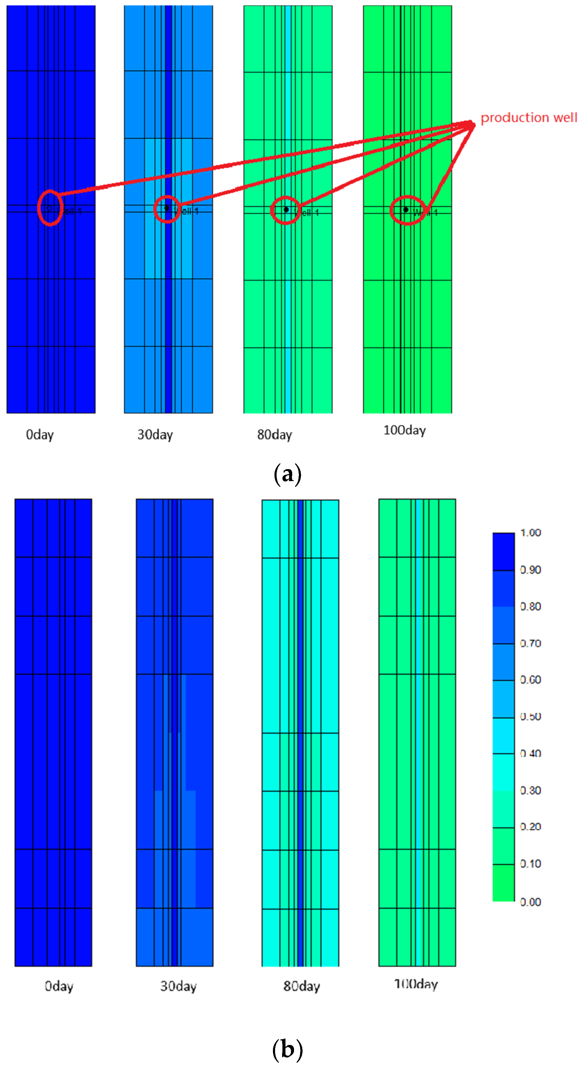
Figure 6 shows the distribution of the fracturing fluid inside the fracture system at different times after 100 days of production. The distribution of the fracturing fluid in the fracture system in the near-well area during production from day 0 to day 100 shows that the fracturing fluid content inside the NFs in the area near the wellbore decreases significantly from day 0 to day 30, while the fracturing fluid content inside the HFs is still high. During the production period from day 30 to day 100, the fracturing fluid content inside the NFs drops to very low values, nearly zero, while a small amount of fracturing fluid is still stored inside the HFs, except near the wellbore. Almost all of the fracturing fluid inside the fracture system in the near-well area returns to the surface. As for the far-well area, it can be seen that the fracturing fluid content inside the NFs decreases significantly during production up to day 80, while the fracturing fluid content inside the HFs is still high. By the 100th day of production, the fracturing fluid content inside the NFs is almost zero, while the fracturing fluid content inside the HFs is still high. For the near-well area, the fracturing fluid inside the fracture system is returned to the surface through the wellbore in a short time. In the far-well area, due to the good connectivity between the fractures, the fracturing fluid inside the NFs is transported to the HFs with high conductivity and then flows back to the surface.

4.3. Low-Fracture-Connectivity Reservoir Production

In actual reservoir development, on the one hand, the number of “connected fractures” formed at the end of hydraulic fracturing to connect HFs and NFs is low due to poor reservoir geology and construction methods. On the other hand, NFs opened by fracturing fluid support are closed due to the lack of propping by the proppant. These reasons lead to poor connectivity between NFs and HFs. NFs and HFs are often connected to each other by only a small number of fractures or are even unconnected. The fractures are independent of each other, making it difficult to form a fracture network with very high conductivity. The fracturing fluid is trapped inside the fracture and has difficulty flowing back to the surface. The permeability of fractures in different directions can characterize the flow ability of the fluid in that direction. A higher permeability indicates that the fluid flows more easily in this direction, which means that the fracture connectivity is better in that direction. Conversely, a lower permeability indicates that the fracture is less well connected in that direction.

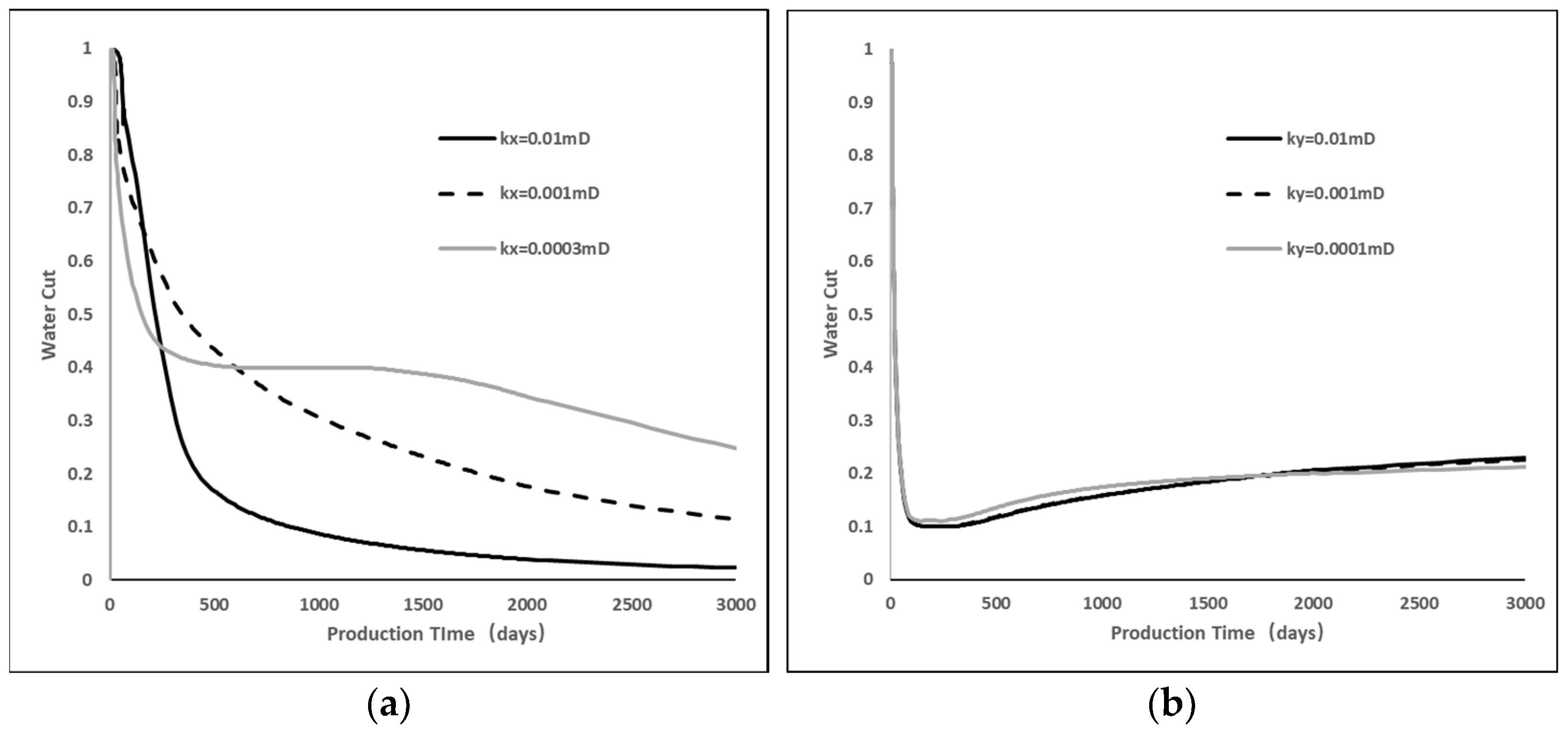
Figure 7 shows the variation curve of the water cut with time during the development of production for 3000 days by controlling the permeability in different directions. By comparing the two curves, it can be seen that controlling the permeability of NFs in the I-direction can significantly affect the change in the water cut in the production process, and it is reflected in the fact that the lower the permeability of NFs in the I-direction, the slower the decrease in water content in the production process. On the other hand, controlling the permeability of natural fractures in the J-direction does not contribute much to the variation in the water cut.

The natural fractures in the I-direction can be seen as “connected fractures” inside the fracture network, as the fractures extend in the plane perpendicular to the I-direction. Reducing the permeability of the natural fractures in the I-direction reduces the connectivity of the “connected fractures”, resulting in weaker fluid communication within the hydraulic fractures. And the degree of closure of the connection fractures can influence the change in the water cut during the production process. The closure of connected cracks can promote the stabilization of the water cut. In the production phase, the early-production fluid is almost entirely water. The water cut decreases with production in a very short period of time, after which the water cut is maintained for smooth production.

For highly connected reservoirs (Figure 5), the fracturing fluid flows back to the surface in a very short time, and the late-production fluid contains almost no water. For most of the reservoirs, the fracture network is poorly connected, the fractures are not sufficiently connected to each other, and a large amount of fracturing fluid is trapped in the HFs and NFs. The fracturing fluid flowback can be divided into two stages (Figure 8):

• The fracturing fluid inside the HFs can quickly flow back to the surface because the fractures are often not effectively connected to each other. Due to the high HF conductivity, the fracturing fluid inside the HFs can quickly flow back to the surface, resulting in a rapid decrease in the water cut.
• The NFs and HFs are connected by only a small number of fractures, and the fracturing fluid in the natural fractures slowly flows back to the surface with production. The water cut is stable during this process. The fracturing fluid trapped inside the NFs plays an important role in stabilizing water production in the later stages of production.

4.4. Stress Sensitivity

In this section, the trend of permeability with the effective stress in natural fractures as well as in hydraulic fractures in the model is set according to the data measured in the previous experiments (Figure 4). Assuming that the reservoir is highly stress-sensitive, the natural fractures are fully supported and fully connected to the hydraulic fractures at the end of fracturing, and the permeability of the natural fractures and hydraulic fractures varies with decreasing effective stress according to the trend in Figure 4. Figure 9 shows the comparison with the low-stress-sensitivity reservoir for 3000 days of production.

The analysis of the production data shows that as production proceeds, the oil rate in the highly sensitive reservoir is higher in the weakly sensitive reservoir under the same development conditions. As for water production, the daily water production in the low-sensitivity reservoir is higher in the pre-production period, while after a period of production, the daily water production in the highly sensitive reservoir drops steeply, and the water production rate decreases continuously with time, and in the late production period, the produced fluid is almost all oil and almost no water. In contrast, for reservoirs with different sensitivities, the water cut in high-sensitivity reservoirs decreases more slowly than in low-sensitivity reservoirs. After 1000 days of production, the water cut of the low-sensitivity reservoir has dropped to below 20%, while the water content of the high-sensitivity reservoir is still above 30%. After a long period of production (3000 days), almost all the fracturing fluid in the low-sensitivity reservoir returned to the surface, with a return rate close to 100%, while the return rate of the high-sensitivity reservoir was 66%, and about 1/3 of the fracturing fluid was still retained inside the reservoir.

Figure 9 and Figure 10 illustrate the distribution of the stagnant fracturing fluid within the high- and low-stress-sensitivity reservoirs from the beginning of production to the final stage (3000 days). The analysis of the distribution of the fracturing fluid inside the fracture system of high- and low-stress-sensitivity reservoirs shows that after a long period of production, almost no fracturing fluid is retained in the low-stress-sensitivity reservoir. A large amount of fracturing fluid is still retained inside the NFs of the high-stress-sensitivity reservoir, and there is almost no fracturing fluid in the HFs.

For the hydraulic fracturing of highly stress-sensitive reservoirs, most of the fracturing fluid is injected into NFs, and a small percentage is retained inside HFs. The fracturing fluid inside the HFs is quickly returned to the surface with production, while a portion of the fracturing fluid inside the natural fractures is slowly returned to the surface through unclosed connecting fractures via hydraulic fractures, a process that helps maintain stable water content during production. A portion of the fracturing fluid is locked inside the natural fractures and has difficulty returning to the surface, resulting in a low drainage rate in the shale reservoir. For the hydraulic fracturing of highly stress-sensitive reservoirs, most of the fracturing fluid is injected into NFs, and a small percentage is retained inside the HFs. The fracturing fluid inside the HFs quickly flows back to the surface with production, while a portion of the fracturing fluid inside the natural fractures is slowly returned to the surface through unclosed connecting fractures through the HFs. This process helps to maintain a stable water content during production. A portion of the fracturing fluid is locked inside the NFs and has difficulty flowing back to the surface, resulting in a low flowback rate in the shale reservoir.

Chen et al. [21] used numerical simulation to study the process of throughput operation and found that it is important to consider unsupported fracture and dynamic fracture inflow capacities. The scenario considering unsupported fractures has higher throughput than the scenario considering only supported fractures, a result similar to that of our study; however, the study of the fracturing fluid distribution was not accurately investigated by numerical simulation. Nur et al. [22] suggested that the utilization of choke management slowed down early oil production, which is most worthwhile in terms of the net present value (NPV). Due to stress sensitivity, the production pressure drop should be reduced in the early stages of production to increase the final production through spontaneous seepage, where a large amount of fracturing fluid is absorbed by the matrix. In our study, it can be seen that, without considering spontaneous seepage and suction, the fracturing fluid is retained inside the fracture system due to poor interconnectivity, and it is difficult for the fracturing fluid inside the supported open fracture system to return.

4.5. Capillary Forces

Shale reservoirs have special physical properties, and their capillary forces are generally higher than those of conventional reservoirs. During the flowback after hydraulic fracturing, a large amount of fracturing fluid seeps into the interior of the matrix and stays inside the reservoir for a long time. The capillary force function (Figure 11) of the matrix is set according to Equation (1), and the capillary forces of the NFs and HFs are neglected.

$$P_{\mathrm{c}}=6.895\times {10}^{-4}\times \frac{\sigma }{a_2{{(\mathrm{S}}_w)}^{a_1}}{\left(\frac{\varphi }{\mathrm{k}}\right)}^{a_3}$$

(1)

The interfacial tension of oil and water (σ) is 30 mN/m. a₁a₂a₃ are constants and take values of 1.86, 6.42, and 0.5.

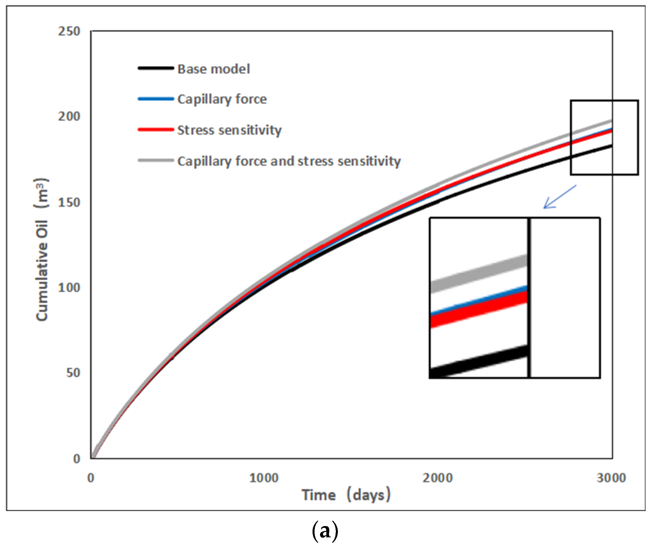
To investigate the extent of capillary forces in shale reservoirs for reservoirs with different sensitivities, Figure 12 comprehensively analyzes the impact of capillary force and stress sensitivity on production.

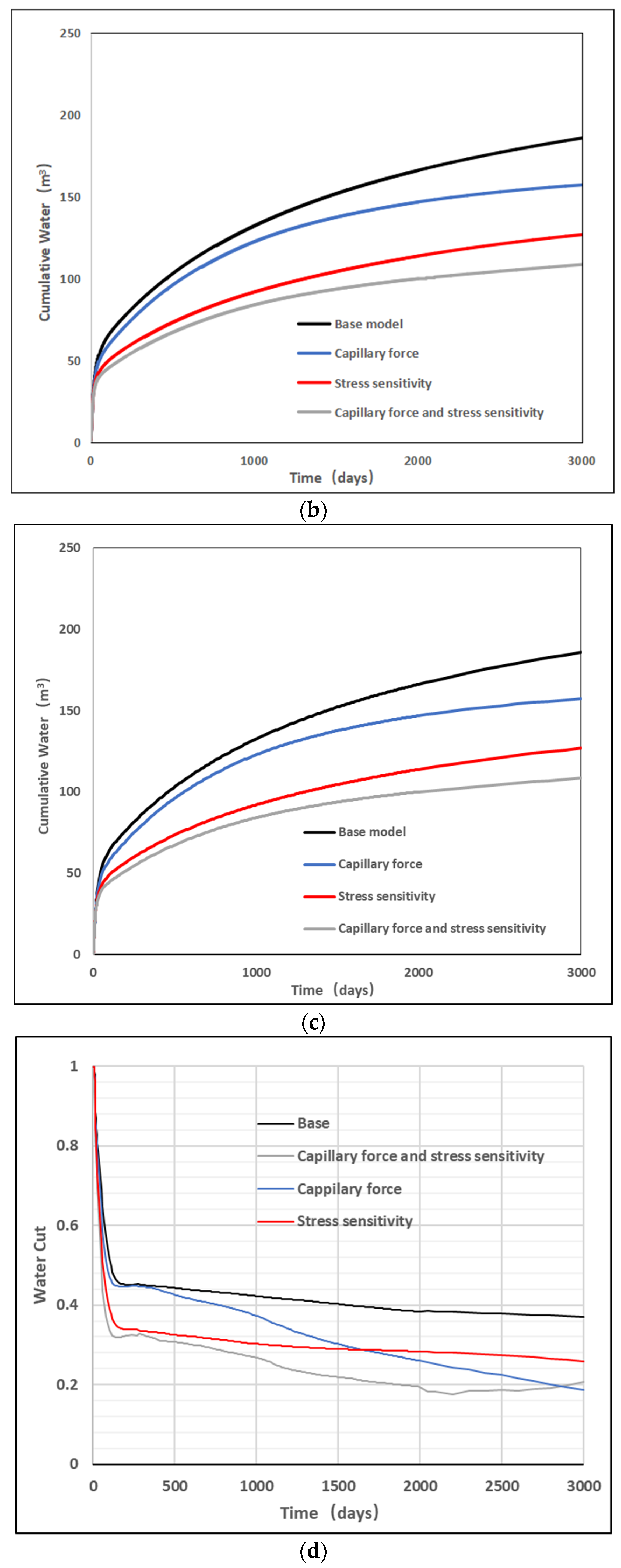
A comparison of the two conditions without capillary forces (black and blue lines) shows that the cumulative water production decreases over 3000 days of production; however, cumulative oil production rises when taking into account the effect of capillary forces. This is mainly due to the fact that the fracturing fluid is continuously transported to the matrix and exchanged for oil under the action of capillary forces. A comparison of the changes in the two curves in (d) shows that there is little difference between development with and without capillary forces in the early production period, but the difference gradually becomes obvious in the middle and late production stages. When the well is opened for production after fracturing, the fracturing fluid in the hydraulic fracture is discharged back to the surface in a short period of time, and there is little difference between the two processes with and without gross tubular force reservoirs. The fracturing fluid inside the natural fracture is slowly discharged back to the surface in the later development process, and part of the fracturing fluid is continuously transported to the matrix interior under the action of capillary forces, which leads to a decrease in the water cut.

The gray line indicates that under the comprehensive analysis of stress sensitivity and the influence of capillary forces, compared with the basic model, cumulative oil production decreases while cumulative oil production increases. This is mainly due to the decrease in the fracture network conductivity of sensitive reservoirs with oil and gas production, leading to a decrease in oil production. However, in the long-term development process, due to the storage of fracturing fluid inside the natural fracture network, a portion of the fracturing fluid seeps into the matrix and is exchanged, resulting in an increase in oil production. Additionally, due to the presence of more fractures that continuously close due to production in sensitive reservoirs, capillary forces have a greater impact on sensitive reservoirs. Therefore, the influence of capillary forces has a greater impact on sensitive reservoirs. From the comparison of the red and blue lines in (c), it is found that the reduction in fracturing fluid return is higher in reservoirs considering only fracture sensitivity than in reservoirs considering only capillary forces. That is to say, under the conditions of this simulation, the contribution of fracture sensitivity to the fracturing fluid reservoir is higher than that of capillary forces.

However, for producing wells in the same area, there can be significant differences between their water cuts during production. It can be hypothesized from the previous simulation that the closure of the fracture system may lead to a difference in water production in the production wells. For wells with sufficiently connected fracture systems, the fracturing fluids are discharged back to the surface within a short period of time after the opening of the wells, which leads to lower water production rates in the later smooth water production period. For reservoirs with more closed fracture systems, the fracturing fluid is locked inside the fractures, and this part of the fracturing fluid is slowly discharged back to the surface, which ensures stable water production in the late stage of production. The water production rate in the stable water production period is the average water saturation of the region.

4.6. Shut-In Time

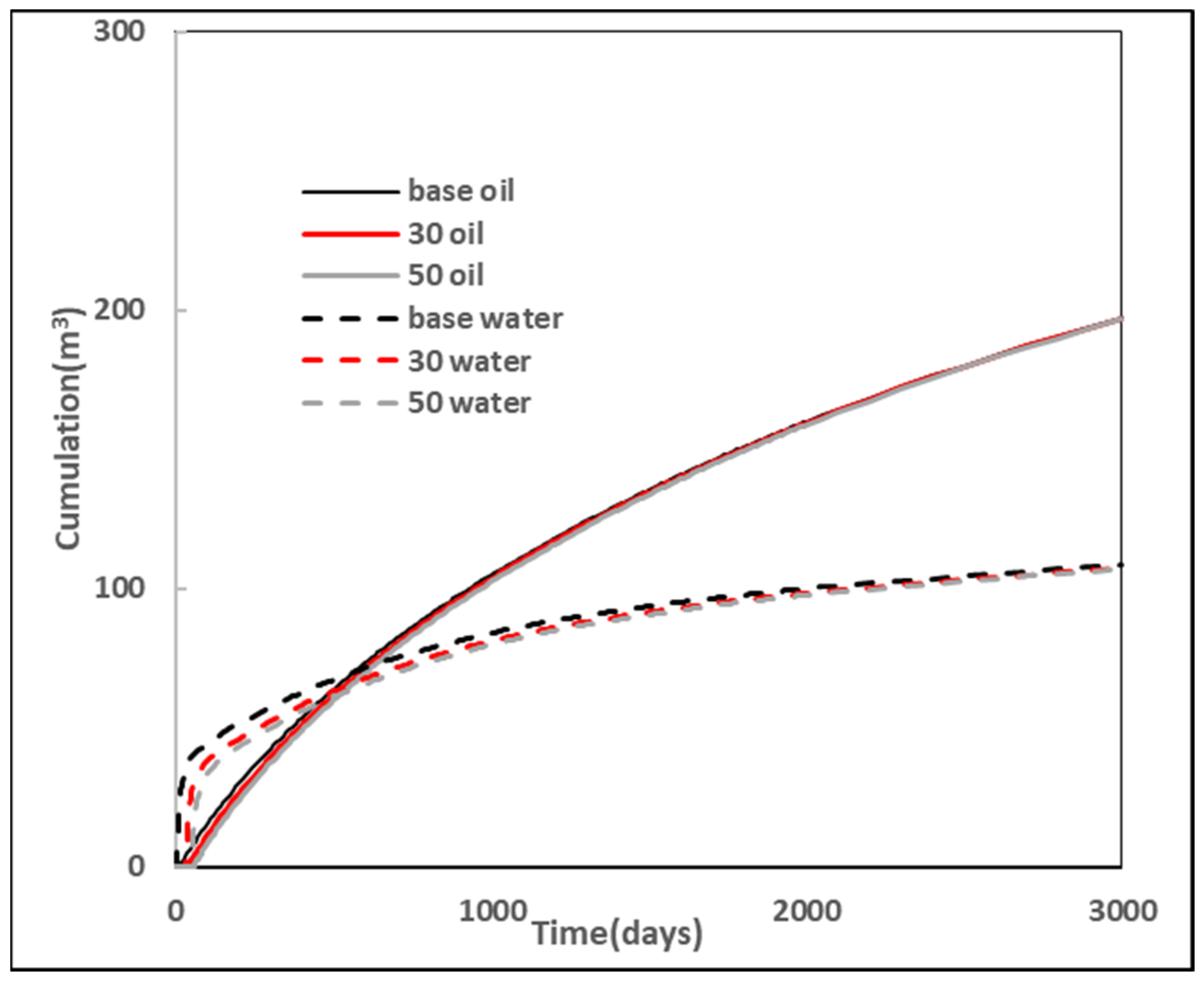
During construction, the wells are usually shut in for a period of time and then opened for production. In order to analyze the influence of extending the shut-in time on development, the shut-in time was set to 0, 30, and 50 days, and the production results for 3000 days of development are shown in Figure 13.

As can be seen from the curves, in the case of a longer production period (3000 days), extending the shut-in time makes little difference in terms of cumulative production, while, in the early period, it is possible to obtain a short period of higher production to compensate for the loss of production due to shut-in during the plugging period. However, all things considered, the impact of a choke on production during the production period is minimal, and an early start-up of the well can be considered to the extent that production conditions allow.

4.7. Discussion

The morphology of the fracture network changes over time after the fracturing of shale reservoirs, resulting in a large number of differences in the way that fracturing fluids are stored. In general, the connectivity of the fracture seam network causes the SRVs formed after hydraulic fracturing to retain a portion of the fracturing fluid. Figure 5, Figure 6 and Figure 7 illustrate the effect of fracture network connectivity on the flowback of fracturing fluids. For reservoirs with high connectivity, the flowback of fracturing fluids is accomplished in a short period of time, and the fracturing fluids injected into the surface can flow back to the surface in a very short period of time. For reservoirs with low connectivity, the I-direction fracture, which is a connectivity fracture, affects the fracturing fluid drainage. For low-connectivity reservoirs, fracturing fluid drainage is a long-term process, and there is a phase of stable water content during the drainage process. In fact, increasing the number of propped fractures may be a possible way to improve the flowback rate.

However, in the study of fracture sensitivity in the current study (Figure 10), it was found that the distribution of fracturing fluids in highly sensitive reservoirs has areas of high water content within the natural system. Contrary to Figure 6, even near the wellhead, there is still a high-water-content area, which means that the fracturing fluid is locked near the wellhead, and this process can explain the low rate of fracturing fluid return in shale reservoirs from one point of view. However, the same region can also be explained by the difference in the water cut due to fracture sensitivity, and the same region has wells with different water cuts. This can also support, from a theoretical point of view, the phenomenon found in Bakken, Eagle Fold, and Permian by Frank’s [23] research.

In previous studies, more attention has been paid to the spontaneous seepage of capillary forces, leading to more fracturing fluid storage. However, in our study, we comprehensively analyzed the effects of capillary forces as well as stress sensitivity on the return of the fracturing fluid (Figure 12). It can be seen that the presence of capillary forces leads to fracturing fluid storage; however, the presence of capillary forces is not the whole reason for fracturing fluid storage. The role of capillary forces is more pronounced in highly sensitive reservoirs compared to normal reservoirs. In a highly sensitive reservoir, more of the fracturing fluid is stored in the fracture network, leading to more spontaneous sorption by the matrix. This leads to stronger spontaneous seepage. Capillary force seepage causes water absorption mainly from inside the natural fractures. In the process of considering the extension of the shut-in time, it was found that it did not have a significant effect on the production of oil, which is also consistent with the findings of Nur et al. [24], and the setting of the shut-in time should be considered comprehensively during the construction of the well.

Our results show that fracture closure due to stress sensitivity causes more retention of the fracturing fluid. After the fracturing fluid is injected into the underlying formation, a portion of the fracturing fluid is supposed to flow from the interconnected fractures to the wellbore and then back to the surface. However, due to the elevated closure stress, a portion of the fracturing fluid is retained inside the fracture system, which may also be an important reason for the low flowback rate. However, it can be hypothesized that the presence of a fracture system plays an important role in the reservoir of fracturing fluids and the contribution of water content during subsequent rejection.

5. Conclusions

• The effective stress rises due to a reservoir pressure drop during reservoir production, resulting in a significant decrease in fracture flow conductivity. For hydraulic fractures, due to the support of the proppant, the decline is significantly lower than that for natural fractures, with a difference of two orders of magnitude.
• For reservoirs with highly connected fractures, the fracturing fluid will flow back to the surface in a short period of time, and the production fluid in the later stage is almost devoid of water. For most reservoirs, the connectivity of the fracture network is poor, and the connectivity between fractures is insufficient, resulting in a large amount of fracturing fluid being trapped inside the fracture system.
• During the production process of sensitive reservoirs, fractures continue to close, and their connectivity decreases. As production progresses, they are locked inside the fracture network. This part of the fracturing fluid ensures a stable water cut in the later stage of production.
• The suction effect of capillary forces can also lead to the retention of the fracturing fluid, and the retention effect of the fracturing fluid is more obvious for sensitive reservoirs. Shut-in wells can increase early production, but the impact on long-term production is not significant.