Abstract
In this paper, the voltage regulation in power systems is addressed from the perspective of the modern paradigm of control logic supported by phasor measurement units. The information available from measurements is used to better adapt the regulation actions to the actual operation point of the system. The use of the online measurement data allows for identifying the sensitivity matrix and for improving the regulation performances with respect to the fast load variations that increasingly affect modern power systems. With the aim of estimating the sensitivity matrices, a preliminary action is necessary to reconstruct the phases of the network voltages, which are assumed not to be provided by the phasor measurement units. This allows for obtaining a model-free adaptive control method. It is then shown how the regulation problem can be formulated in terms of a linear quadratic Gaussian problem, properly considering the load modeling in terms of the stochastic Ornstein–Uhlenbeck process. This control strategy has the advantage of avoiding dangerous oscillations of power flows, as demonstrated through the results of some simulations on a classical test network. Particularly, the advantage of the proposed approach is shown in the presence of different levels of load disturbances.
1. Introduction
The voltage control service in power systems is implemented through the coordination of local resources and loads to counteract the load variations and the intermittent generation of renewable sources [1]. The modern evolution of loads and generation in power systems is driving novel regulation strategies based on the use of phasor measurement unit (PMU) technology, which allows for fast and accurate estimating of power systems’ dynamics [2]. PMUs are largely used in power systems [3], and their use has been investigated with respect to voltage regulation [4]. Extensive use of data available in real time from PMUs requires stochastic approaches tailored to manage large datasets to be used for the identification of the correct system state and to provide proper countermeasures to the sudden changes that could arise. Moreover, the increasing penetration of small-sized renewable generation units progressively implies an increasing number of resources to control. This can potentially lead to local negative effects on system dynamics. Focusing on secondary voltage control (SVC), in [5], a linear quadratic integral regulator is proposed, which aims to avoid undesired voltage oscillation due to the presence of numerous controllable sources. Load fluctuation [6] and load disturbance [7] have also been identified as issues that can negatively affect voltage control, thus suggesting improved control strategies using PMUs.
While the use of data available from PMUs or other measurement systems [8] is becoming increasingly popular, the importance of proposing control strategies properly tailored to manage the large availability of this data has arisen as a critical issue. Based on the concept of data-driven, innovative methods exploiting model-free control and adaptive control approaches have recently been proposed in the literature [9]. A data-driven control method is proposed in [10], which exploits the PMU data to realize an online adaptive coordination design of decentralized SVCs. An SVC is proposed in [11] based on the virtual reference feedback tuning approach, which is an off-line data-driven method. In [12], the PMU data are used in the SVC by defining an optimal control model that aims to minimize the worst-case load voltage change. This last approach is improved in [13] with a maximum likelihood approach to account for measurement uncertainties. A two-step approach based on the expectation–maximization probability theory is used in [14] to consider the stochastic measurement error within the SVC. PMU data are also used to estimate the system state without requiring any model knowledge. In [15], a linear regression of reactive power observations and the application of a weighted least square is used to estimate the dynamic load time constants, which, in turn, allows for estimating the sensitivity matrices of the system. The control method proposed in [7] adopts a non-linear constrained optimization problem combined with a worst-case design technique to elaborate the regulation actions driven by the PMU-based estimation of the load variations. In [16], the power system is regarded as a stochastic dynamic system with loads modeled according to the Ornstein–Uhlenbeck (OU) process and sensitivity matrices estimated through linear regression analysis. The OU process, in fact, allows for the accurate modeling of the stochastic dynamics of the power system [17], with particular emphasis in case it is required to model randomness due to renewable energy resources and innovative loads present in modern power systems [18].
The significance of using PMUs to estimate the sensitivity matrices is that they avoid having detailed and complete knowledge of the network topology and model parameters. This, indeed, is not possible in real-world applications, especially when dealing with modern systems characterized by a high share of renewables [19]. The estimation of sensitivity matrices based on PMU data is basically related to the voltage phase angle recovering. Thus, in [20], a method based on the phase retrieval problem is proposed. Phase retrieval was proposed within a multidisciplinary context devoted to the phase estimation problem of a complex signal given a design matrix and based on the observation of real-valued magnitude measurements [21]. The classical phase retrieval problem is formulated as a quadratic optimization problem with complex decision variables and known design matrices. In power system applications, the design matrix is the system Jacobian matrix, which is assumed to be unknown. In this case, in [20], it has been adopted based on the PhaseCut algorithm [22].
In this paper, a novel SVC strategy is applied based on an adaptive model-free approach driven by PMU data. Based on the available measurements, the proposed approach estimates the system sensitivity matrices through the phase retriever approach; then, based on the OU process, a proper linear quadratic controller is proposed. More in detail, the OU formulation suggests using a linear quadratic Gaussian control (LQGC), which allows us to directly include the load disturbance within the SVC loop, thus enabling proper control actions to improve the system dynamics against disturbances and the fast variations in the loads. In that regard, the system dynamics, including LQGC, is formulated in terms of stochastic equations, which include a Gaussian random process, and a quadratic cost criterion is properly formulated to identify a feedback controller within the control loop.
The main contributions of this paper refer to the proposal of the SVC strategy, which includes (i) the use of the phase retriever for the estimation of the sensitivity matrices, thus making the control adaptive and model-free, (ii) the formulation of a proper control strategy based on the LQGC driven by the OU stochastic load power model, and (iii) the derivation of the control scheme which properly integrates the LQGC within the classical SVC scheme for the evaluation of the control signals used to counteract load variations due to the disturbances.
The rest of this paper includes, in Section 2, a brief survey on the sensitivity matrices for the SVC problem and some details on their estimation through the phase retriever approach. In Section 3, the formulation of the LQGC applied to the SVC is presented, and its integration within the control scheme is proposed. Section 4 deals with the estimation of the stochastic disturbance parameters affecting the load power. Results of some numerical applications on a classical test network are presented and discussed in Section 5. These results clearly show the accuracy of the estimation method pursued through the OU multivariate process, for which a metric has been appropriately defined. Also, they prove the effectiveness of the proposed improved control strategy for lowering voltage fluctuations as a consequence of load disturbances. Some conclusions and future perspectives are reported in Section 6.
2. Sensitivity Matrices for Secondary Voltage Control
In this section, the derivation of the sensitivity matrices for SVC is performed. Particularly, they are formulated in a proper form to be used within the phase retrieval problem, whose solution allows us to obtain the data-driven derivation of the matrices. This enables the proposal of a free-model approach for the SVC based on the data available from PMU measurements.
Sensitivity matrices of the SVC can be identified through the linearized model of the power system, which is summarized by the following well-known model:
where is the load-flow Jacobian.
The model can be conveniently split as follows:
From the (2) we obtain
By substituting (4) in (3), we have
In order to simplify the notation, the following matrices are defined:
Thus, (5) can be rewritten as
Equation (8), assuming , can be split as
In the context of the SVC, reference is made to a different form of sensitivity relations, where the output variables are the reactive generation powers and the load voltages; the magnitudes of the generation voltages are regarded as input variables, and the load powers as disturbances. Thus, to obtain a more suitable set of equations, it is possible to derive by inverting (10) as follows:
Hence, by substituting it in the (9), we obtain
In order to simplify the notation, the following matrices are then introduced:
Thus, we obtain the set of Equations (11) and (12) in a more compact form as follows:
The sensitivity matrices have to be estimated on the basis of the available measurements of the active and reactive powers and voltage magnitudes, having assumed the unknown network modeling. However, the complication arises that, in general, the knowledge of the phases is not guaranteed, and, therefore, it is necessary to solve the problem of reconstructing the phases starting from the available measurements. This problem can be formulated as the following minimization problem:
where and are the active and reactive power injection measurements, and is the voltage magnitude measurement.
For this purpose, the Lemma 1 in [22] comes to help by providing the expressions in closed form of and , as follows:
The value is obtained by solving the minimization problem (15), subject to the constraints (16). To simplify the notation, the following matrices are now defined:
Equation (15) can then be rewritten as
The calculation of the null points of the derivative function now arises:
By inverting the second equality of the Equation (19), it is possible to obtain the expression as
It is worth noting that based on the available measurements from PMUs, the phases can be evaluated according to (20), thus allowing for the derivation of the sensitivity matrices of the network, which can be used for the purpose of the SVC.
The derivation of the sensitivity matrices can be then pursued through the following online procedure:
- -
- the vectors of measurements of the active powers () and reactive powers (), as well as the vector of the measurements of the voltage magnitude (), are sent to the control center;
- -
- the vectors , , , and are derived through (17);
- -
- the vector of the estimated voltage phases are evaluated through (20);
- -
- Jacobian matrix and in turn the sensitivity matrices are derived from (1).
Through an online PMU-based monitoring system, the proposed approach is then able to adapt the SVC in real time to the actual structure and operation point of the system so that the advantages in terms of quality of services clearly emerge in systems characterized by highly intermittent loads and generation units.
3. Secondary Voltage Regulation as Linear Quadratic Gaussian Integral Regulator
In this section, a quadratic optimal controller with counteracting action to the effect of load variations on the busbars’ voltages is proposed. For this purpose, the LQGC is used, which is a method based on the separation between state estimates and optimal controllers [23]. The solution to the linear quadratic problem is to utilize an observer-based controller and a linear quadratic regulator. Their combination allows for handling the problem of regulation of linear systems with disturbance factors with Gaussian statistical properties. In our proposal, driven by the observation given by the PMU measurements, the OU process is used to model the disturbances affecting the loads.
The proposed controller is an LQGC based on an augmented state-space with the aim of including the integral of error and disturbance modeling in the solution. Here, the disturbance is not measured; thus, the proposed controller is applied together with the OU stochastic process to model the load variations, whose parameters are estimated starting from the knowledge of the information made available by the PMUs.
The basic state variable vector includes the voltage variation at the generation buses, whereas the control vector is the vector of variations in the reference stator voltages of the generators.
First of all, dynamic modeling has to be tailored to identify a proper control strategy. This can be inferred by describing the primary voltage control dynamics by a convenient matrix , which is chosen to realize the first-order model of the controlled excitation systems. Furthermore, an integrator is introduced in the control scheme for canceling the steady state error between the steady state value of and its reference . This is performed by defining the new state variable :
The considered dynamic model can be summarized as
which can be written in a more compact form as
where , and . The control strategy has to be performed by optimizing the reactive power sharing between the various power plants. A classical strategy is the one referring to the following constrained minimization problem:
where is the reactive power of the ith generator, and is the total reactive power variation requested by the SVC. This criterion of assigning the reactive power to each generator can be performed by minimizing the following index:
where is a proper diagonal matrix, whose elements are generator-rated powers. This can be pursued in a deterministic way by considering the first of (14), where and are equal to zero. Based on the optimal control approach, proper weight matrices and can, hence, be introduced for considering the cost related to the control effort:
The values of the and matrices are chosen to guarantee that the eigenvalues of the overall dynamic matrix are all real to avoid the onset of insidious inter-area oscillations. Furthermore, it is guaranteed that there is the desired distribution of reactive powers among the various machines [5]. In [5], the solution of this problem is analytically solved in the case of a linear quadratic control. Herein, the load variation effect is investigated and, more specifically, its incidence on the voltage profile is modeled as a multivariate OU process:
where and are the variations in the active and reactive powers; and are the Wiener processes of the active and reactive power variations. The matrices and are diagonal, assuming that the loads are independent of each other, and they are called rates of mean reversion. The OU stochastic process was first introduced to overcome the physical inconsistency of the Wiener process for describing the velocity of a Brownian motion. Firstly, it has to be highlighted that the Wiener process trajectories have a behavior that tends to spread up over time because of the process variance increasing over time, while the OU ones are confined near the origin due to the action of the mean reversing time. Furthermore, by examining the two-sided spectrum of the OU, when , one can observe that this stochastic process can be regarded as a filtered white noise. More specifically, it exhibits the behavior of a Wiener process for high frequencies, i.e., for short observation time, while for low values of frequency, corresponding to long observation time, it behaves as a white phase noise [24]. This characteristic makes it very interesting for many physical stochastic phenomena and, in particular, for the power system loads.
Based on the (28) and (29), it is derived that the OU processes can be added through the augmented state variable vector, :
with , , , .
which can then be written in the matrix form as
thus, the augmented state space model can be obtained as follows:
In order to have a more compact form, the augmented matrices , , and can be defined as
The augmented space state model is then summarized as
where , and is the augmented matrix .
The corresponding control scheme is reported in Figure 1. In the control scheme, the gain parameters and are evaluated according to the LQGC, whose tuning depends on the estimation of the stochastic disturbances’ parameters. This estimation can be performed by starting from the knowledge of dynamic load data, which is described in the following section.
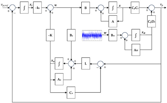
Figure 1.
Control scheme of the SVC with stochastic input and .
The stability of the controlled system relies on the well-known property that the eigenvalues are those of the dynamic matrices and , which are intrinsically stable because they derive from the LQR control and the Kalman filter.
4. Estimation of the Stochastic Disturbance Parameters
The loads are modeled as the multivariate OU process reported in (28) and (29), thus obtaining the augmented state space model (32). Hence, the considered state space model includes the augmented state variable vector; is modeled according to the multivariate OU process (31). In order to estimate the multivariate OU process, we start from the notation adopted for stochastic differential equations [25]:
where, according to (30), accounts for the active and reactive load powers’ variations; the elements of matrices and are the rates of mean reversion and standard deviation of the OU process associated with the active and reactive load powers’ variations with Wiener processes , as assumed in (28) and (29).
By the integration of (36), it is obtained as follows:
where is the vector of independent normally distributed random variables with covariance . To simplify the notation, we can use the exponential matrix of the mean regressions rates and the covariance matrix , thus obtaining the following equation:
For our purposes, it is interesting to estimate the parameters of the statistical process starting from a vector of observations, i.e., the PMU measurements, assuming that it is an OU process.
Regarding the statistical process given by , the result is a zero-mean process with the same exponential matrix and the estimates of and the covariance matrix provided by [25]:
where the matrices , , and are sufficient statistics for the matrices and , equal to
From (38), it is obvious that the matrices and can eventually be estimated as
The estimation and can be used in (31)—and, in turn, in the augmented state space model (32)—which is useful in incorporating the load disturbance counteracting function within the SVC.
5. Simulations
The proposed SVC is applied to the test network shown in Figure 2, which is the classical WSCC 9-bus test network at 230 kV, 60 Hz [26]. The data of the network are reported in Appendix A. Three power plants are supposedly connected to the network:
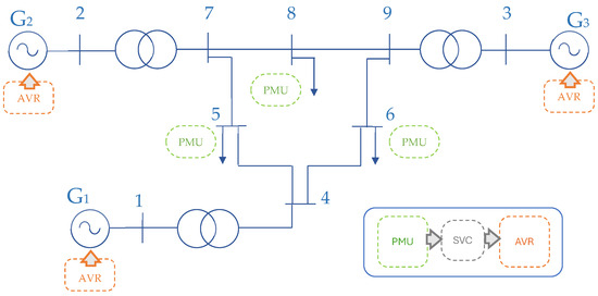
Figure 2.
Test network.
- -
- bus #1: 247.5 MVA-rated power at 16.5 kV generator equipped with a transformer having of 5.76%;
- -
- bus #2: 192 MVA-rated power at 18 kV generator equipped with a transformer having of 6.25%;
- -
- bus #3: 128 MVA-rated power at 13.8 kV generator equipped by a transformer having 5.86%.
Three loads are connected to the buses #5 (125 MW/50 MVAR-rated power), #6 (90 MW/30 MVAR-rated power), and #8 (100 MW/35 MVAR-rated power). Based on the approach proposed in [27], the pilot bus #4 is identified. A PMU is supposed to be connected at each load bus. They communicate their measurements to an SVC center, which elaborates the information and sends the reference signals to the automatic voltage regulators of the generators, as depicted in the flow chart reported in Figure 2. Regarding the communication between the various PMUs, it can be performed in different ways, such as fiber optic, 5G, etc. The better method to exchange data can be selected by considering the presence of a preexisting communication grid and the location of each PMU.
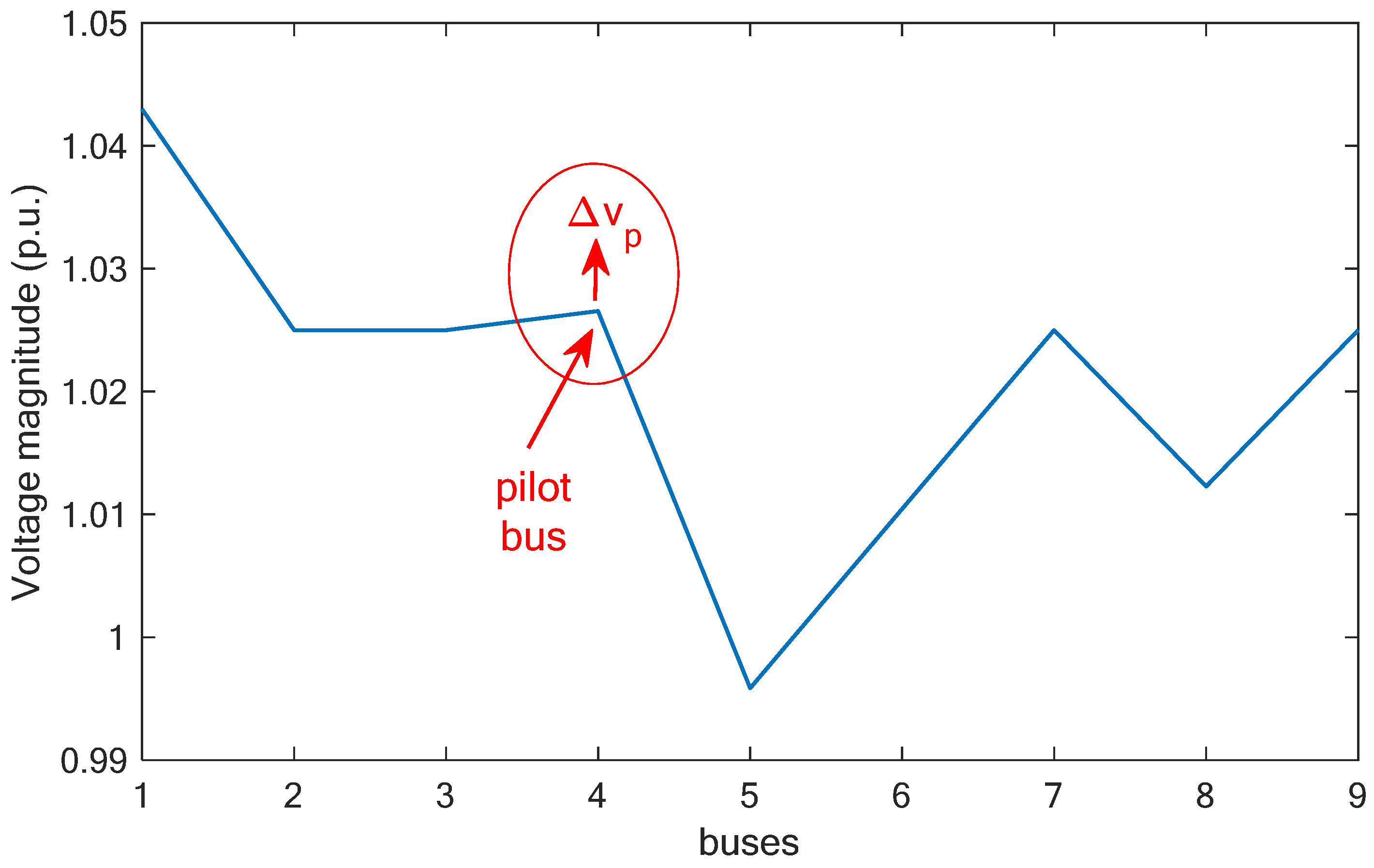
The initial operation point of the network is supposed to correspond to the steady state operation point with the reference voltage value assigned at the generation buses #1, #2, and #3 of 1.043 p.u., 1.025 p.u., and 1.025 p.u., respectively. Bus #1 is assumed to be a slack bus, and the generators of buses #2 and #3 inject active powers of 1.63 p.u. and 0.85 p.u. A load flow analysis has been performed, which provided the magnitudes of the voltages reported in Figure 3. In the figure, the pilot bus is highlighted, together with an increment , which is the aim of this application.

Figure 3.
Voltage magnitudes at the network buses.
Still referring to the steady state condition, the first generator injects 0.72 p.u. of active power, while the reactive powers delivered by the three generators are 0.31 p.u., −0.057 p.u., and −0.22 p.u.. Based on the Jacobian matrix, the sensitivity matrices are derived as follows:
The effectiveness of the multivariate process estimation procedure of the loads is tested considering matrices and for the stochastic modeling of the three loads:
Then, the Bayesian estimation procedure summarized in is applied in the simulations with different observation time intervals. By way of example, the estimated matrices and with an observation time interval equal to :
Once these two matrices are known, the and matrices could be estimated according to the (42) and (43) as
The relative error has been calculated for and as the ratio of the Euclidean norm of the deviation matrix and the Euclidean norm of the original matrix:
These percentage errors for the two matrices, and , have been evaluated for an observation time of s and correspond to and 0.38%.
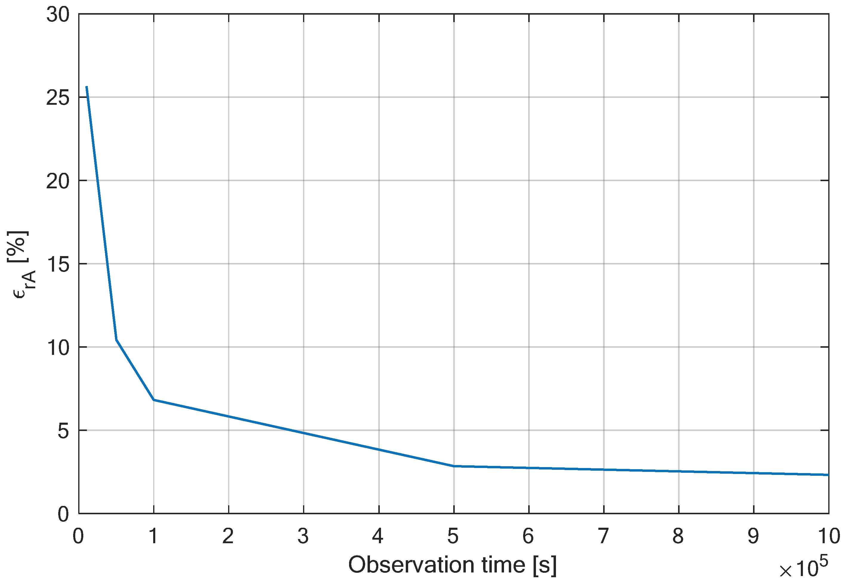
In order to better clarify the effect of the sampling time interval length, a sensitivity analysis has been performed to analyze the percentage error for an increased length of the observation time, i.e., the number of samples available from the PMU data, keeping constant the time interval length . In this case, the error trends of and are reported in Figure 4 and Figure 5, respectively. The considered observation time ranges from s to s.
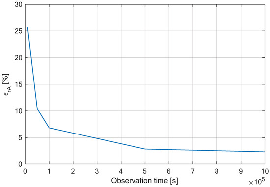
Figure 4.
Percentage relative error trend in the .
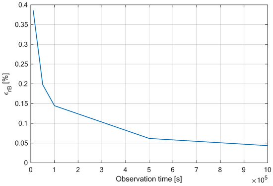
Figure 5.
Percentage relative error trend in the .
As shown in Figure 4 and Figure 5, the errors affecting and decrease when the observation time length increases. Particularly, these errors with the larger observation time reach the values of 2% for and 0.04% for . This is because while observation time increases, the length of time interval is kept constant and, consequently, the number of samples increases, thus providing a larger set of observation data that provide more accurate estimations. The increased accuracy of the estimation versus the increased length of the observation time demonstrates the robustness of the proposed estimation model.
Once the accuracy of the estimation approach is based on the multivariate OU process driven by the PMU data, the proposed SVC strategy is applied to the test network of Figure 2. For this purpose, starting from the steady state condition represented by the voltage profile shown in Figure 3, a load disturbance represented by the matrices and (46) and (47) is supposed. Then, a reference voltage profile at the pilot bus p.u. is imposed.
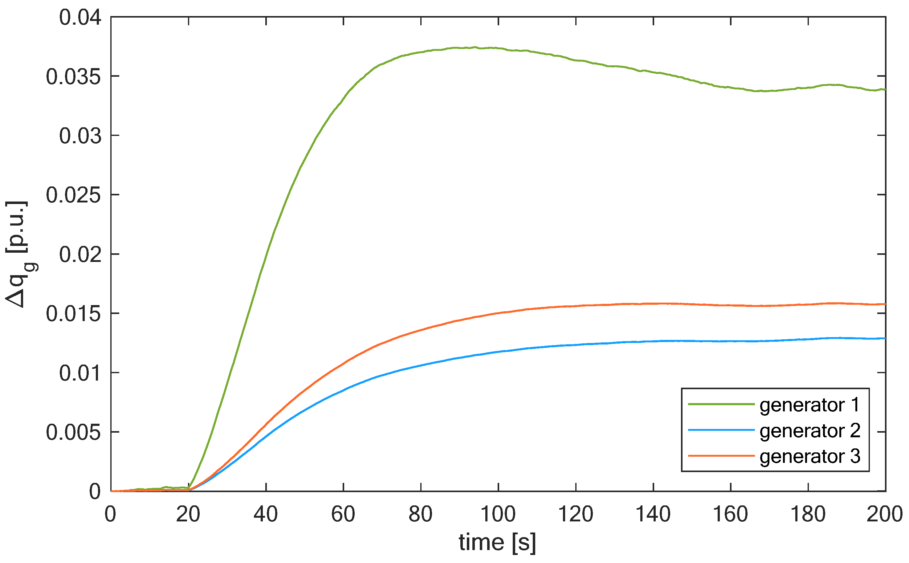
The response of the proposed SVC in terms of voltage profile at the pilot bus is shown in Figure 6, together with the reference step voltage variation. The corresponding generators’ reactive powers are reported in Figure 7.
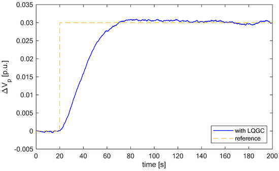
Figure 6.
Voltage profile at the pilot bus in the case of step reference value of 0.03 p.u.
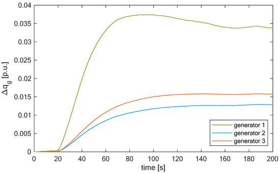
Figure 7.
Generators reactive power variation in the case of p.u.
The profile of the magnitude variation in the pilot bus voltage (Figure 6) shows that the proposed SVC method provides effective performances by limiting the effect of the load disturbances while preserving the main role of the SVC, which is the modification of the pilot bus voltage according to the desired step variation imposed by the reference value. The effect of LQGC makes the response time slightly faster than the response time of conventional SVC. This change is performed thanks to the reactive power support of the generators, whose variations are expected to be feasible, as shown in Figure 7.
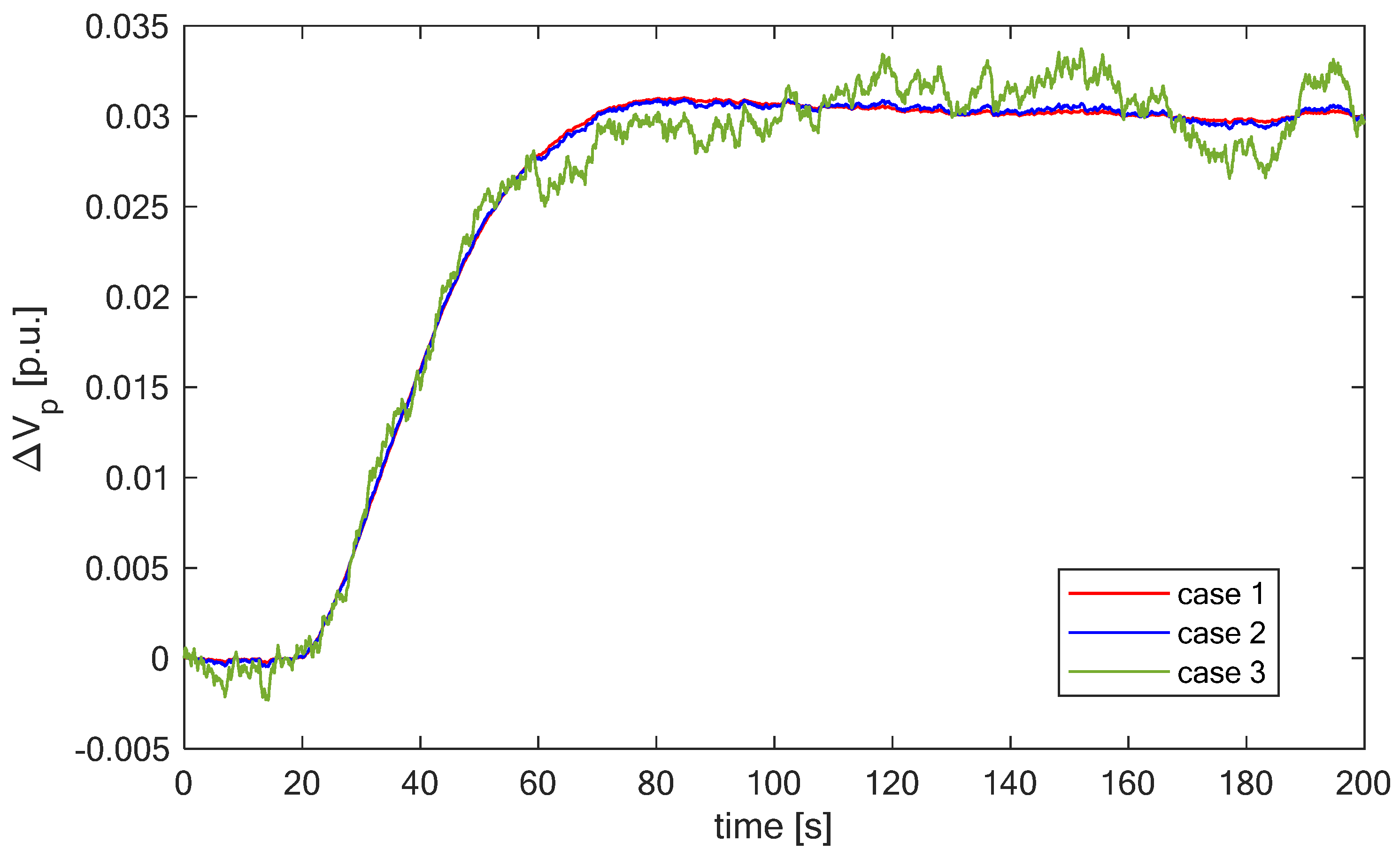
In order to better show the effect of load disturbances, different noise levels are considered in the following three study cases:
- Case 1
- Case 2
- Case 3
In Figure 8, the voltage trends for the three cases are reported. As clearly highlighted in the figure, the response of the proposed SVC in terms of the pilot bus voltage profile is very satisfactory in cases 1 and 2. When noise increases in Case 3, the procedure is also able to contain fluctuations even though they are obviously more evident than in the other cases.
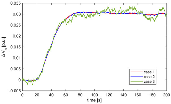
Figure 8.
Comparison of voltage profiles for three noise levels.
For the sake of completeness, a different step variation is also imposed on the reference pilot bus voltage, corresponding to the decrement p.u. The response of the pilot bus voltage is shown in Figure 9.
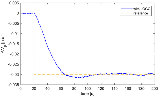
Figure 9.
Voltage profile at the pilot bus in the case of p.u.
The profile of Figure 9 shows that the good performance of the proposed SVC is also confirmed in the case of negative step variation in the reference voltage at the pilot bus. Indeed, the voltage follows the reference value in a proper way, while lowering the fluctuations due to the load disturbances.
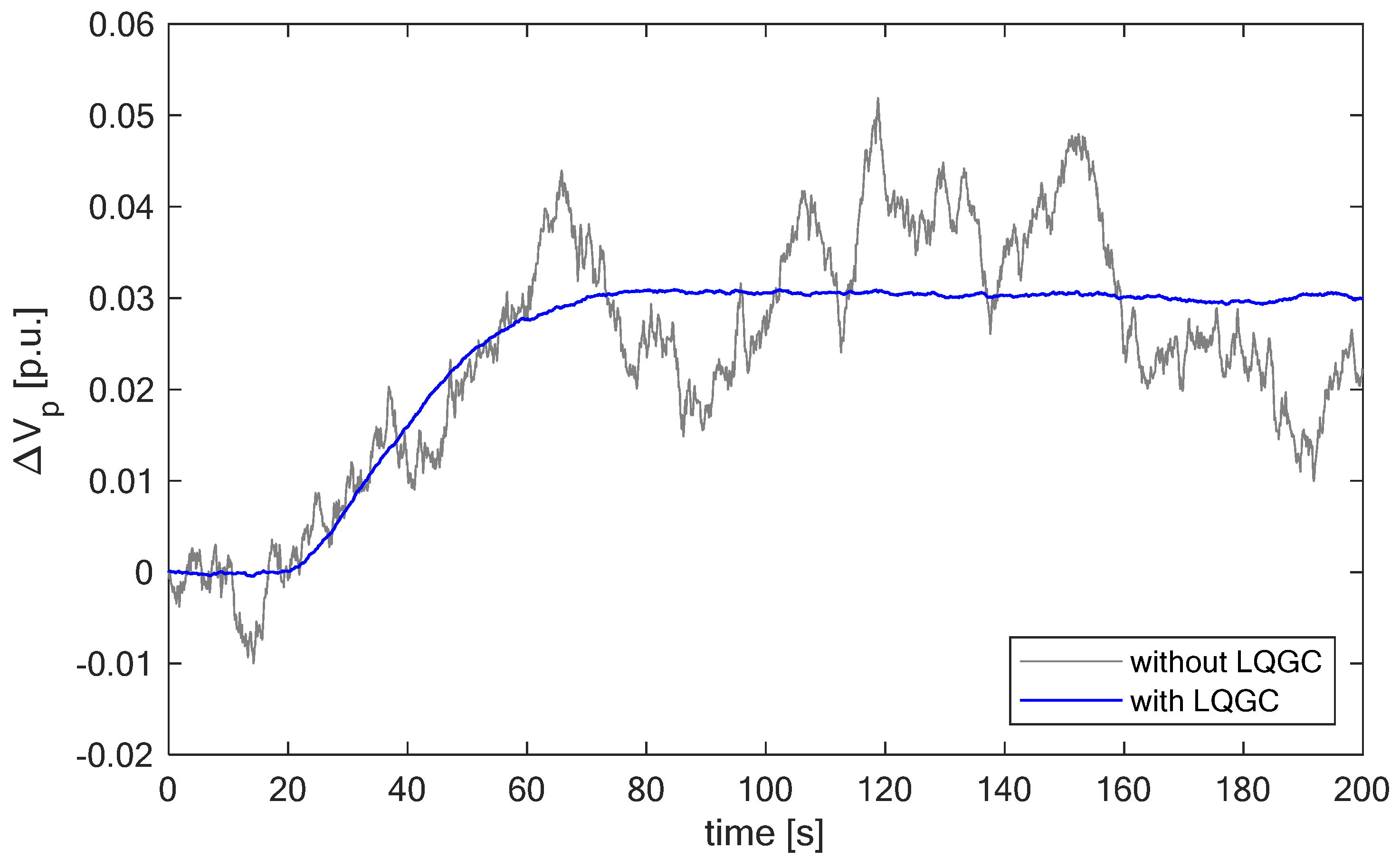
In order to analyze the improvements obtained by the proposed approach compared to the conventional SVC method, a comparison between the responses in terms of pilot voltage profile obtained through the proposed approach and that obtained through the LQI-based approach [5] is reported in Figure 10. The comparison refers to the case when load powers are affected by the noises of Case 2.

Figure 10.
Voltage profile comparison at the pilot bus using LQGC and LQI.
In Figure 10, the differences in terms of pilot voltage profiles between the two methods clearly appear. The differences are due to the fact that conventional methods do not account for load power affected by noises. Although the rising time is similar in both cases, it has to be noted that the LQI-based approach resulted in an overshoot greater than 30% compared to the 3.3% implied by the LQGC, whereas the pilot bus voltage fluctuation around its reference value has standard deviation of 0.01 p.u. compared to 6.2∙10−4 of the LQGC.
6. Conclusions
The problem of secondary voltage control is addressed in this paper. While this task is traditionally faced with controllers with excellent performance, the increasing penetration of resources of an intermittent nature, including both generation units and loads, requires focusing on some issues related to the fluctuation of power, which potentially can worsen the level of secure operation. The proposed approach explores the use of a modern paradigm of control logic supported by phasor measurement units to provide improved regulators that can counteract the oscillations in voltages consequent to the load disturbances and the modifications of the operation point of the system. An online measurement system is supposed to provide a set of data in real time that is used to identify the sensitivity matrices of the system and to improve the regulation performances to face the fast load variations. More in detail, for the purposes of estimating the sensitivity matrices, it is shown that it is preliminary needed to reconstruct the phases of the network voltages. Then, the regulation problem is properly formulated in terms of a linear quadratic Gaussian problem, in which the load variations are modeled according to the stochastic Ornstein–Uhlenbeck process. The proposed approach has been demonstrated to be effective and robust through some simulation on a classical test network. In this regard, the accuracy of the proposed estimation model has been clearly evidenced by highlighting that the error is decreasing while increasing the available data from the measurement system. Also, the result of the numerical application shows that the control strategy has the advantage of avoiding dangerous oscillations while preserving the traditional performance of the secondary voltage regulators aimed at modifying the bus voltages according to the operational needs. The main findings of the numerical application clearly reveal the effectiveness of the proposed approach in reducing voltage fluctuations due to the load power disturbance of different levels of noise. In this regard, the proposed approach has been demonstrated to be able to provide very satisfactory performances even in the presence of severe disturbances, for which the voltage fluctuations at the pilot buses are contained within acceptable ranges. Moreover, the advantages of the proposed approach, compared to the conventional methods when load disturbances are present, have been clearly demonstrated through comparative analysis. Future research activities should be devoted to the identification of proper allocation methods for phasor measurement units, which can help find the best buses where information on loads can be caught.
Author Contributions
Conceptualization: E.C., D.L., M.F. and D.V.; methodology: E.C., D.L., P.D.P. and F.M.; software: D.L., P.D.P. and F.M.; validation: E.C., D.L., M.F., D.V., P.D.P. and F.M.; formal analysis: E.C., D.L., M.F. and D.V.; investigation: E.C., D.L., M.F., D.V., P.D.P. and F.M.; data curation: E.C., D.L., P.D.P. and F.M.; writing—original draft preparation: E.C., D.L., P.D.P. and F.M.; writing—review and editing: E.C., D.L., M.F., D.V., P.D.P. and F.M.; visualization: P.D.P. and F.M.; supervision: D.L. and D.V. All authors have read and agreed to the published version of this manuscript.
Funding
This research received funding from Project “NEST–Network 4 Energy Sustainable Transition—Spoke 7 (Smart Sector Integration)”, CUP E63C22002160007, funded by the European Union as part of the NextGenerationEU plan through the National Recovery and Resilience Plan (NRRP).
Data Availability Statement
The data that support the simulations are detailed in the text.
Conflicts of Interest
The authors declare no conflicts of interest.
Appendix A
In Table A1, the data of the lines of the test network are summarized (base power 100 MW). Nominal values of the load power are reported in Table A2.

Table A1.
Data of the lines.
Table A1.
Data of the lines.
| Lines | Resistance (p.u.) | Reactance (p.u.) | Susceptance (p.u.) | |
|---|---|---|---|---|
| From Bus | To Bus | |||
| #4 | #5 | 0.0100 | 0.085 | 0.176 |
| #4 | #6 | 0.0170 | 0.092 | 0.158 |
| #5 | #7 | 0.0320 | 0.161 | 0.306 |
| #6 | #9 | 0.0390 | 0.170 | 0.358 |
| #7 | #8 | 0.0085 | 0.072 | 0.149 |
| #8 | #9 | 0.0119 | 0.101 | 0.209 |
Table A2.
Nominal power of the load.
Table A2.
Nominal power of the load.
| Bus # | #5 | #6 | #8 |
| Active power (MW) | 125 | 90 | 100 |
| Reactive power (MVAR) | 50 | 30 | 35 |
References
- Sun, H.; Guo, Q.; Qi, J.; Ajjarapu, V.; Bravo, R.; Chow, J.; Li, Z.; Moghe, R.; Nasr-Azadani, E.; Tamrakar, U.; et al. Review of Challenges and Research Opportunities for Voltage Control in Smart Grids. IEEE Trans. Power Syst. 2019, 34, 2790–2801. [Google Scholar] [CrossRef]
- Pazderin, A.; Zicmane, I.; Senyuk, M.; Gubin, P.; Polyakov, I.; Mukhlynin, N.; Safaraliev, M.; Kamalov, F. Directions of Application of Phasor Measurement Units for Control and Monitoring of Modern Power Systems: A State-of-the-Art Review. Energies 2023, 16, 6203. [Google Scholar] [CrossRef]
- Aminifar, F.; Fotuhi-Firuzabad, M.; Safdarian, A.; Davoudi, A.; Shahidehpour, M. Synchrophasor Measurement Technology in Power Systems: Panorama and State-of-the-Art. IEEE Access 2014, 2, 1607–1628. [Google Scholar] [CrossRef]
- Abdalla, O.H.; Fayek, H.H.; Abdel Ghany, A.M. Secondary Voltage Control Application in a Smart Grid with 100% Renewables. Inventions 2020, 5, 37. [Google Scholar] [CrossRef]
- Lauria, D.; Mottola, F.; Giannuzzi, G.; Pisani, C. An advanced secondary voltage control strategy for future power systems. Int. J. Electr. Power Energy Syst. 2024, 156, 109734. [Google Scholar] [CrossRef]
- Ge, H.; Guo, Q.; Sun, H.; Wang, B.; Zhang, B.; Wu, W. A Load Fluctuation Characteristic Index and Its Application to Pilot Node Selection. Energies 2014, 7, 115–129. [Google Scholar] [CrossRef]
- Su, H.-Y.; Kang, F.-M.; Liu, C.-W. Transmission Grid Secondary Voltage Control Method Using PMU Data. IEEE Trans. Smart Grid 2018, 9, 2908–2917. [Google Scholar] [CrossRef]
- Di Palma, P.; Collin, A.; De Caro, F.; Vaccaro, A. The Role of Fiber Optic Sensors for Enhancing Power System Situational Awareness: A Review. Smart Grids Energy 2024, 9, 1–26. [Google Scholar] [CrossRef]
- Gong, X.; Wang, X.; Cao, B. On data-driven modeling and control in modern power grids stability: Survey and perspective. Appl. Energy 2023, 350, 121740. [Google Scholar] [CrossRef]
- Zhao, Y.; Lu, C. An Adaptive Coordinated Secondary Voltage Control with PMU Data. In Proceedings of the 2018 IEEE Power & Energy Society General Meeting (PESGM), Portland, OR, USA, 5–10 August 2018; pp. 1–5. [Google Scholar] [CrossRef]
- Nascimento, M.M.; Bernardo, R.T.; Dotta, D. Data-Driven Secondary Voltage Control Design using PMU Measurements. In Proceedings of the 2020 IEEE Power & Energy Society Innovative Smart Grid Technologies Conference (ISGT), Washington, DC, USA, 17–20 February 2020; pp. 1–5. [Google Scholar] [CrossRef]
- Su, H.-Y.; Liu, C.-W. An Adaptive PMU-Based Secondary Voltage Control Scheme. IEEE Trans. Smart Grid 2013, 4, 1514–1522. [Google Scholar] [CrossRef]
- Su, H.-Y.; Liu, T.-Y. Enhanced Worst-Case Design for Robust Secondary Voltage Control Using Maximum Likelihood Approach. IEEE Trans. Power Syst. 2018, 33, 7324–7326. [Google Scholar] [CrossRef]
- Liu, J.-H.; Li, Z.-H. Robust Expectation-Maximization-Based Secondary Voltage Control Scheme Considering Stochastic Measurement Error. IEEE Trans. Power Syst. 2023, 38, 2958–2961. [Google Scholar] [CrossRef]
- Pierrou, G.; Lai, H.; Hug, G.; Wang, X. A Decentralized Wide-Area Voltage Control Scheme for Coordinated Secondary Voltage Regulation Using PMUs. IEEE Trans. Power Syst. 2024, 39, 7153–7165. [Google Scholar] [CrossRef]
- Pierrou, G.; Wang, X. An Online Network Model-Free Wide-Area Voltage Control Method Using PMUs. IEEE Trans. Power Syst. 2021, 36, 4672–4682. [Google Scholar] [CrossRef]
- Pierrou, G.; Wang, X. The Effect of the Uncertainty of Load and Renewable Generation on the Dynamic Voltage Stability Margin. In Proceedings of the 2019 IEEE PES Innovative Smart Grid Technologies Europe (ISGT-Europe), Bucharest, Romania, 29 September–2 October 2019; pp. 1–5. [Google Scholar] [CrossRef]
- Verdejo, H.; Awerkin, A.; Kliemann, W.; Becker, C. Modelling uncertainties in electrical power systems with stochastic differential equations. Int. J. Electr. Power Energy Syst. 2019, 113, 322–332. [Google Scholar] [CrossRef]
- Yuan, Y.; Low, S.H.; Ardakanian, O.; Tomlin, C.J. Inverse Power Flow Problem. IEEE Trans. Control. Netw. Syst. 2023, 10, 261–273. [Google Scholar] [CrossRef]
- Talkington, S.; Grijalva, S. Phase Retrieval via Model-Free Power Flow Jacobian Recovery. In Proceedings of the 14th ACM International Conference on Future Energy Systems (e-Energy ‘23), Orlando, FL, USA, 20–23 June 2023; Association for Computing Machinery: New York, NY, USA, 2023; pp. 510–523. [Google Scholar] [CrossRef]
- Dong, J.; Valzania, L.; Maillard, A.; Pham, T.; Gigan, S.; Unser, M. Phase retrieval: From computational imaging to machine learning: A tutorial. IEEE Signal Process. Mag. 2023, 40, 45–57. [Google Scholar] [CrossRef]
- Waldspurger, I.; d’Aspremont, A.; Mallat, S. Phase recovery, MaxCut and complex semidefinite programming. Math. Program. 2015, 149, 47–81. [Google Scholar] [CrossRef]
- Putri, A.N.; Machbub, C.; Mahayana, D.; Hidayat, E. Data Driven Linear Quadratic Gaussian Control Design. IEEE Access 2023, 11, 24227–24237. [Google Scholar] [CrossRef]
- Bibbona, E.; Panfilo, G.; Tavella, P. The Ornstein–Uhlenbeck process as a model of a low pass filtered white noise. Metrologia 2008, 45, S117–S126. [Google Scholar] [CrossRef]
- Singh, R.; Ghosh, D.; Adhikari, R. Fast Bayesian inference of the multivariate Ornstein-Uhlenbeck process. Am. Phys. Soc. E 2018, 98, 012136. [Google Scholar] [CrossRef] [PubMed]
- Anderson, P.M.; Fouad, A.A. Power System Control and Stability, 2nd ed.; IEEE Press: New York, NY, USA, 2003. [Google Scholar]
- Conejo, A.; de la Fuente, J.I.; Goransson, S. Comparison of alternative algorithms to select pilot buses for secondary voltage control in electric power networks. In Proceedings of the Mediterranean Electrotechnical Conference (MELECON), Antalya, Turkey, 12–14 April 1994; Volume 3, pp. 940–943. [Google Scholar] [CrossRef]


Disclaimer/Publisher’s Note: The statements, opinions and data contained in all publications are solely those of the individual author(s) and contributor(s) and not of MDPI and/or the editor(s). MDPI and/or the editor(s) disclaim responsibility for any injury to people or property resulting from any ideas, methods, instructions or products referred to in the content. |
© 2024 by the authors. Licensee MDPI, Basel, Switzerland. This article is an open access article distributed under the terms and conditions of the Creative Commons Attribution (CC BY) license (https://creativecommons.org/licenses/by/4.0/).