Performance Evaluation of Static and Dynamic Compressed Air Reservoirs for Energy Storage

Abstract

The concept of static and dynamic reservoirs is presented, and their performances are evaluated. The static reservoir is a simple reservoir with constant volume, and the dynamic one has a volume which varies as a function of the position of an internal piston coupled to a spring. The spring is compressed when the pressure in the chamber rises and exerts a proportional force on it. The two reservoirs are components to be used in compressed air energy storage systems. The study comprises a model of the compression machine as well as models of the two reservoirs. The filling processes are simulated, and the different variables are represented as a function of time. A reduced scale experimentation set-up is presented, and its behavior is first simulated. Then. the results are compared to the experimental records.

1. Introduction

In the context of global warming and climate change, alternative energy sources are called upon to replace traditional fossil sources, with the aim of significantly reducing greenhouse gas emissions [1]. Renewable energy sources, with the examples of wind energy or photovoltaic generators, present the character of intermittency and stochastic or unpredictable production and need to be assisted by important energy storage facilities [2,3]. When the possibilities of realizing large pumped hydro storage installations are limited due to geographical and topographical conditions, their energy capacity is, in addition, a limiting factor when compared to the huge demand for electric power across countries or continents [4]. As a possible solution that goes in the same direction as decentralized production [5], local and domestic storage equipment is considered, where smaller units would assume the function of equalizing the power demand and bridge the fluctuations in stochastic production or assume the day-to-night shift of photovoltaic sources. Electrochemical batteries are currently at the top of the list for domestic applications with their high energy density and with a strong trend towards the reduction of acquisition costs. But several concerns remain open regarding the quantity of materials available for mass production and the question of recycling techniques, in relation to the limited number of cycles or even the associated aging phenomena.

A possible alternative to electrochemical batteries is compressed air energy storage (CAES), which has been studied and proposed for large facilities [6,7,8] and for smaller units [9,10,11,12,13]. Due to the limited energy capacity of CAES, even if the storage pressure is of several hundred bar, stationary applications have been considered first. But applications for mobility also have been proposed for a long time, with the example of the Mekarski tramway being one [14]. More recent realizations for individual mobility and short ranges have reached the state of pre-commercialization [15,16,17].

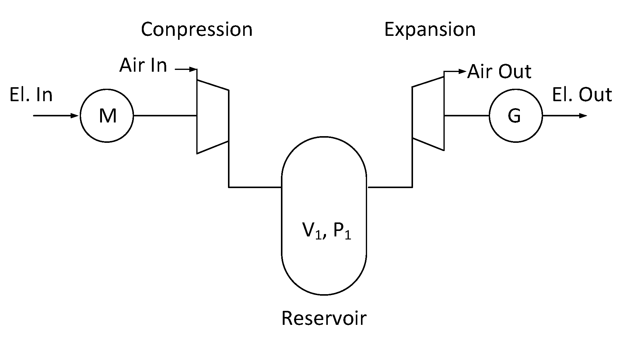
2. Compressed Air Energy System with Accumulation in a Storage Vessel

A conventional compressed air energy storage system is composed of an air compressor feeding a reservoir in the charging mode and of an expansion machine for the discharging mode. The system is completed by an input and an output interface to the electric system, namely a motor driving the compressor and a generator driven by the expansion turbine (Figure 1). The air reservoir represents the accumulating element of the chain and is the object of the present study.

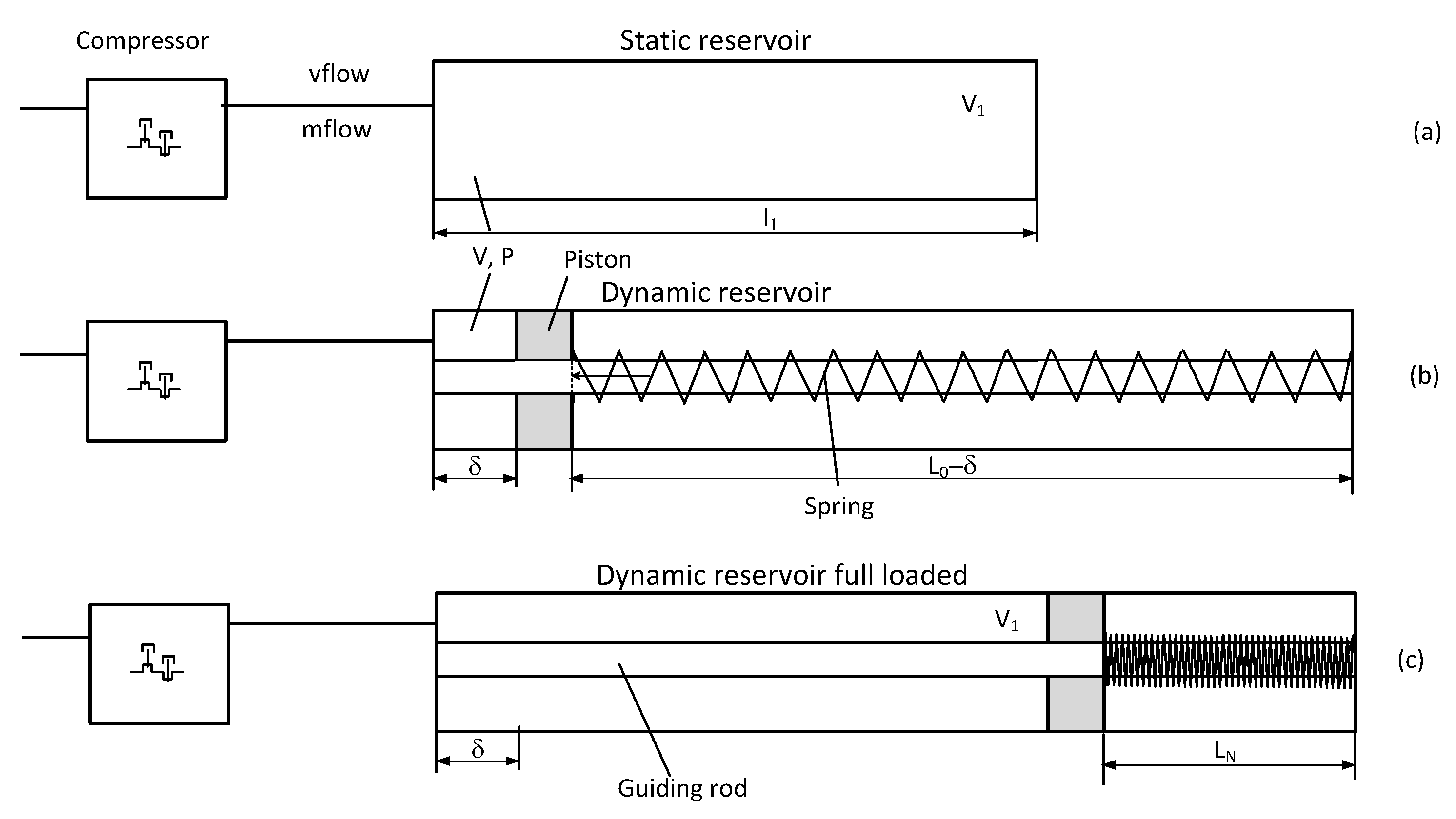
2.1. Static and Dynamic Reservoirs

Two different systems are evaluated. The first uses a reservoir with constant volume. This system is called the static reservoir and is represented in Figure 2a. The second system is a reservoir with variable volume, as proposed in [18]. The variable volume is obtained by a moving piston inside the cylindric reservoir and coupled to a spring. The air injected into the reservoir from the compressor moves the piston and compresses the spring, where an additional amount of energy is stored. This system is called the dynamic reservoir. A schematic representation is given in Figure 2b. Figure 2c shows the same system in the full state of charge, where the space occupied by the spring in its compressed state becomes evident. The two cylindric volumes have the same section. The volume of the dynamic reservoir is equal to the volume of the static reservoir when the position of the piston δ reaches the value of the length l₁ of the static reservoir. When the piston is at this position, the spring exerts a force equal to the pressure P multiplied by the piston’s surface A.

$$F_{spring}=P\cdot A=k\cdot l_1$$

(1)

The pressure P appears in the volume of the cylinder due to the injection of air by the compressor. The pressure depends on the mass of air inside the volume, and its value is given by rel. (2):

$$P=m\cdot {\displaystyle \frac{RT}{V}}$$

(2)

where m is the time integral of the mass flow imposed by the compressor.

$$m={\displaystyle \underset{0}{\overset{t}{\int }}mflow\cdot dt}$$

(3)

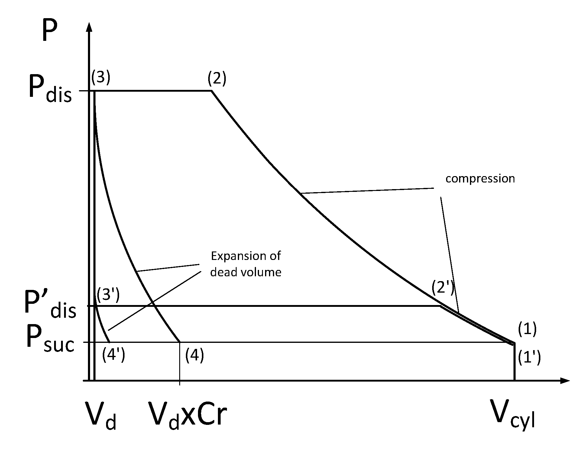
2.2. The Model of the Compressor

The compressor is considered as a source of mass in this modeling. Compressors are usually characterized by their nominal volume flowrate ${\dot{V}}_{nom}$. The nominal volume flow rate ${\dot{V}}_{nom}$ is expressed in m³ per second from its given value in liters per min. The value of 190 l/min is chosen in the considered example and corresponds to the characteristic of the compressor used in the example described in [18].

$${\dot{V}}_{nom}=190 l/\min \cdot {10}^{-3}/60=0.00316 {\mathrm{m}}^3/\mathrm{s}$$

(4)

The real volume flowrate ${\dot{V}}_{real}$ is of a different value due to the effect of the expansion of the dead volume after the end of the discharge, when the piston enters its return stroke. The real volume flowrate is calculated with the help of a so-called volumetric yield ${\eta }_V$ defined as

$${\eta }_V=1-V_r\cdot C_r$$

(5)

where $V_r$ is the ratio of the top volume to the bottom volume of the compression cylinder.

$$V_r=V_{top}/V_{bot}$$

(6)

And $C_r$ is the compression ratio or the ratio of the discharge pressure to the suction pressure. It varies from 1 to $P_{\max }/P_{atm}$ during a full charging process.

$$C_r=P_{dis}/P_{suc}$$

(7)

The real volume flowrate becomes

$${\dot{V}}_{real}={\dot{V}}_{nom}\cdot {\eta }_v={\dot{V}}_{nom}(1-V_r\cdot C_r)$$

(8)

Then, the mass flow rate is calculated as

$$\dot{m}={\dot{V}}_{real}\cdot {\rho }_0$$

(9)

Numerically, the nominal mass flowrate of the example is calculated.

$$\begin{array}{l}{\dot{m}}_{nom}={\dot{V}}_{nom}\cdot {\rho }_0={\displaystyle \frac{190 \mathrm{l}/\min \cdot 0.001 {\mathrm{m}}^3/\mathrm{l}}{60 \mathrm{s}/\min }}\cdot 1.2 {\mathrm{kg}/\mathrm{m}}^3=0.00316 {\mathrm{m}}^3/\mathrm{s}\cdot 1.2 {\mathrm{kg}/\mathrm{m}}^3\\ =0.0038 \mathrm{kg}/\mathrm{s}\end{array}$$

(10)

The effect of the expansion of the dead volume is illustrated by the P-V diagram in Figure 3. The piston of the compressor starts to move from the position with the largest volume (V_cyl = V_bott), and the pressure is equal to P_suc (1), (1′). Then, when the pressure reaches the discharge value (P_dis, P’_dis) (2), (2′), the discharge valve opens, the air is exhausted, and the volume decreases to V_top = V_d. During the return stroke, the suction valve does not open until the pressure of the remaining air in the dead volume falls below the value of the suction pressure P_suc. The effective suction volume becomes

$$V_{cyl}-V_d\cdot C_r$$

(11)

leading to the definition of the volumetric yield ${\eta }_V$.

$${\eta }_V=1-V_r\cdot C_r$$

(12)

2.3. Modeling the Two Reservoirs

2.3.1. Parameters of the Reservoirs

The present paper will first describe the behavior of static and dynamic reservoirs as described in [14]. The parameters of these examples are listed in

Table 1. Parameters of the static and dynamic reservoirs (Ref. [14]).

Static Reservoir
Volume	0.1 m3
Dynamic reservoir
Variable volume	0–0.1 m3
Stroke of the piston	0.9 m
Surface of the piston	0.111 m2
Constant of the spring	61.7 kN/m
Moving mass	10 kg

.

2.3.2. Structural Diagram of the Static Reservoir System

Figure 4 gives the structural diagram of the static reservoir system. The real mass flowrate provided by the compressor is accumulated in the reservoir, which is represented by the time integral (block 1/s). From the accumulated mass of air, the pressure is calculated with an ideal gas law. The actual value of the pressure P_dis is fed back to the calculation of the compression ratio C_r used for the calculation of the volumetric yield.

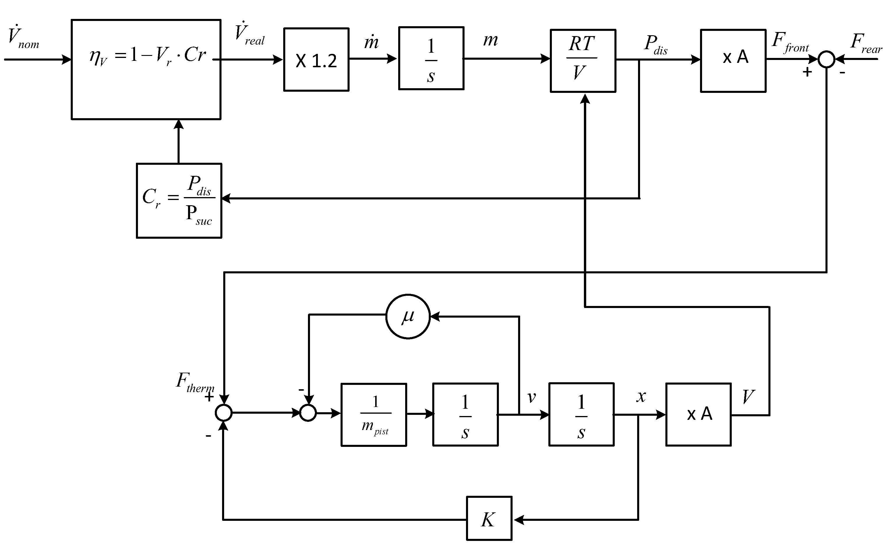
2.3.3. Structural Diagram of the Dynamic Reservoir System

In the dynamic reservoir system, the pressure exerted on the mobile piston by the injected air produces a displacement of it and a compression of the spring. The system comprises two different energy accumulation elements. First, energy is stored in the form of compressed air in the variable volume of the cylinder, and second, in the tension of the spring. The calculation of the piston’s position and of the air accumulation volume is realized according to a dynamic model for the association of the mass of the piston and of the spring. The energy accumulated in the form of compressed air is calculated with the same model as for the static piston system described in the previous section, namely via the accumulated mass of air in the chamber and an associated state equation. In this case, the accumulation volume varies with the position of the piston.

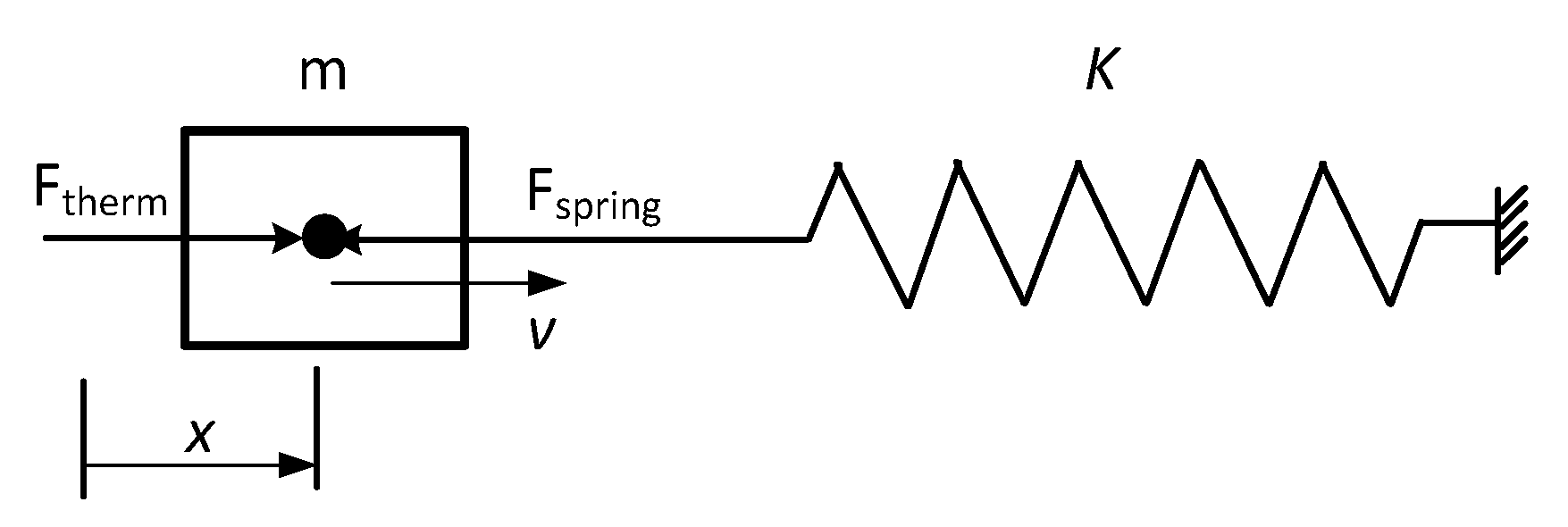
2.3.4. The Model of the Spring–Mass System

The description of the movement of the piston and its impact on the compression of the spring can only be made by using a model based on integral causality [19,20]. So, the piston and the storage spring are modeled as a classical damped mechanical oscillator, as represented in Figure 5. The spring characteristic and the corresponding differential equation can be written as follows:

$$F_{spring}=Kx$$

(13)

$$m\ddot{x}=F_{therm}-Kx-\mu \dot{x}$$

(14)

m is the mass of the mobile piston.

The force caused by a thermodynamic effect F_therm is the difference in the force caused by the pressure in the cylinder’s chamber (absolute value) on the front side of the piston, minus the effect of the atmospheric pressure on the rear side of the piston. K is the spring constant, and μ the velocity-dependent friction coefficient.

The structural diagram of the dynamic reservoir system is given in Figure 6. The compressor model is identical to the model used previously and uses the principle of volumetric yield. The state equation considers the variable volume depending on the piston’s position. The diagram includes the damped mass–spring model. In this model, losses in the spring are modeled through the damping factor μ. Other losses, like friction of the piston on the cylinder walls or on the guiding rod, are not considered. Also, compressibility losses are neglected because of the very slow variation in the pressure and the related slow motion of the piston.

2.4. Energies Accumulated

2.4.1. Volume of Air

The energy content of the volume of air depends on its volume, pressure, and temperature. In the present system, where the piston moves slowly, the thermodynamic phenomenon can be considered as evolving according to an isothermal characteristic. In the full state of charge, the pressure is 6 bar in a volume of 0.1 m³. The corresponding stored energy is calculated as

$$\begin{array}{l}{E}_{stat}=P\cdot V\left(\ln {\displaystyle \frac{P}{P_{atm}}}-1+{\displaystyle \frac{P_{atm}}{P}}\right)=6\cdot {10}^5\cdot 0.1\left(\ln {\displaystyle \frac{6}{1}}-1+{\displaystyle \frac{1}{6}}\right)\\ =6\cdot {10}^5\cdot 0.1\cdot 0.958=57505 \mathrm{J}\end{array}$$

(15)

This value is in the air volume in both cases, constant volume and variable volume when it reaches its maximum (0.1 m³) and when the pressure is identical. The simulation of the charging process presented in the next section will show that this state of the variable volume is reached at t = 340 s that is also the time point at which the pressure of 6 bar is reached. For the constant volume system, the pressure of 6 bar is reached after a time duration of 254 s. This confirms that the spring model and parameters are correct.

2.4.2. Energy Accumulated in the Spring

The energy accumulated in the spring is calculated with usual formulas

$$E_{spring}={\displaystyle \int P}\cdot dt={\displaystyle \int F\cdot \dot{x}\cdot dt=}{\displaystyle \int k\cdot x\cdot \dot{x}\cdot dt}$$

(16)

With

$${(uv)}^{\prime }=u^{\prime }v+{uv}^{\prime },u=v$$

(17)

$${\displaystyle \int {(u\cdot u)}^{\prime }}=u^2={\displaystyle \int u^{\prime }u+{uu}^{\prime }}=2{\displaystyle \int {uu}^{\prime }}$$

(18)

Then

$$E_{spring}=k{\displaystyle \int x\cdot \dot{x}\cdot dt}={\displaystyle \frac{k{x}^2}{2}}$$

(19)

When k = 61.7 kN/m and x = 0.9 m

$$E_{spring}={\displaystyle \frac{k{x}^2}{2}}={\displaystyle \frac{61.7\cdot {10}^3 \mathrm{N}/\mathrm{m}\cdot {(0.9 \mathrm{m})}^2}{2}}=24.9 \mathrm{kJ}$$

(20)

3. Simulation Results

The structural diagrams of the static and dynamic reservoir systems have been implemented in a numeric simulation (Simulink, R2020) and present the evolution of the different variables as functions of time. In the static reservoir, the accumulated mass of air and the pressure in the reservoir are relevant. For the dynamic reservoir, additional variables such as the force exerted on the piston, its displacement, and the variable volume are considered.

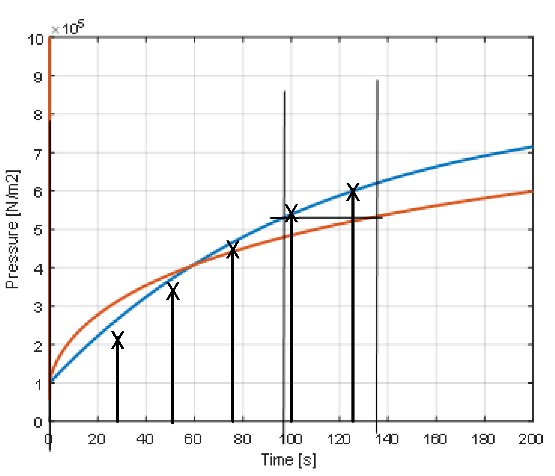
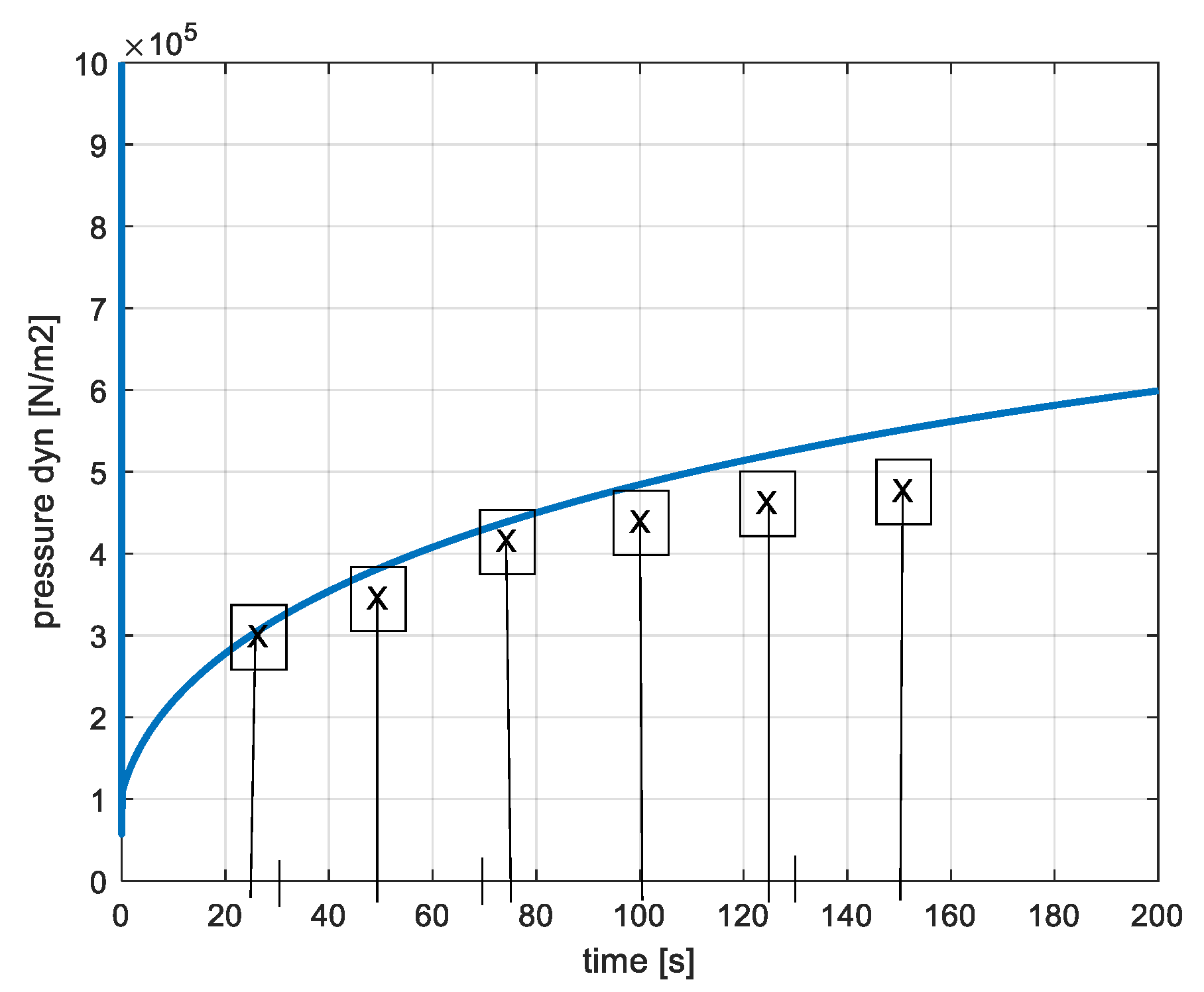
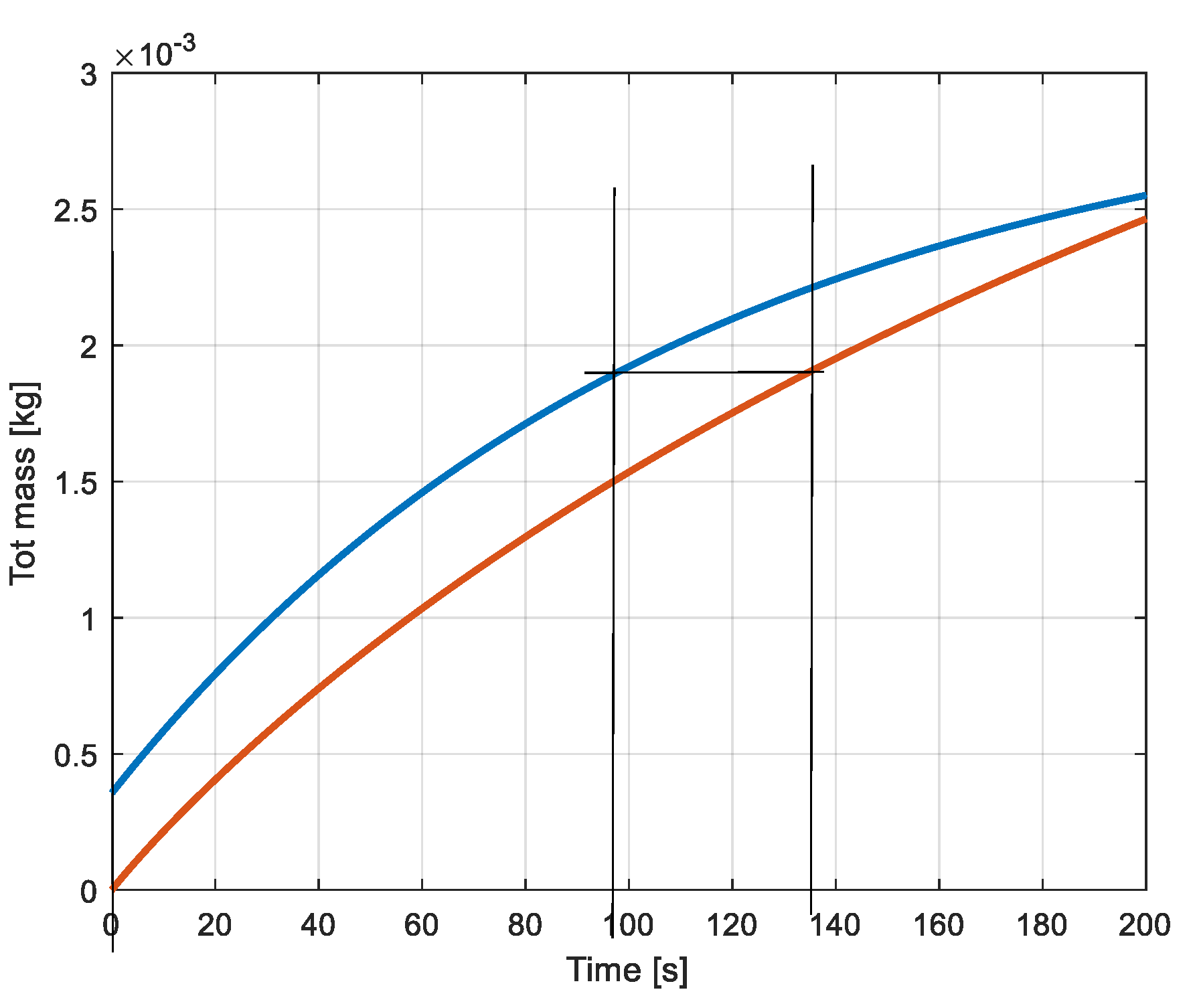
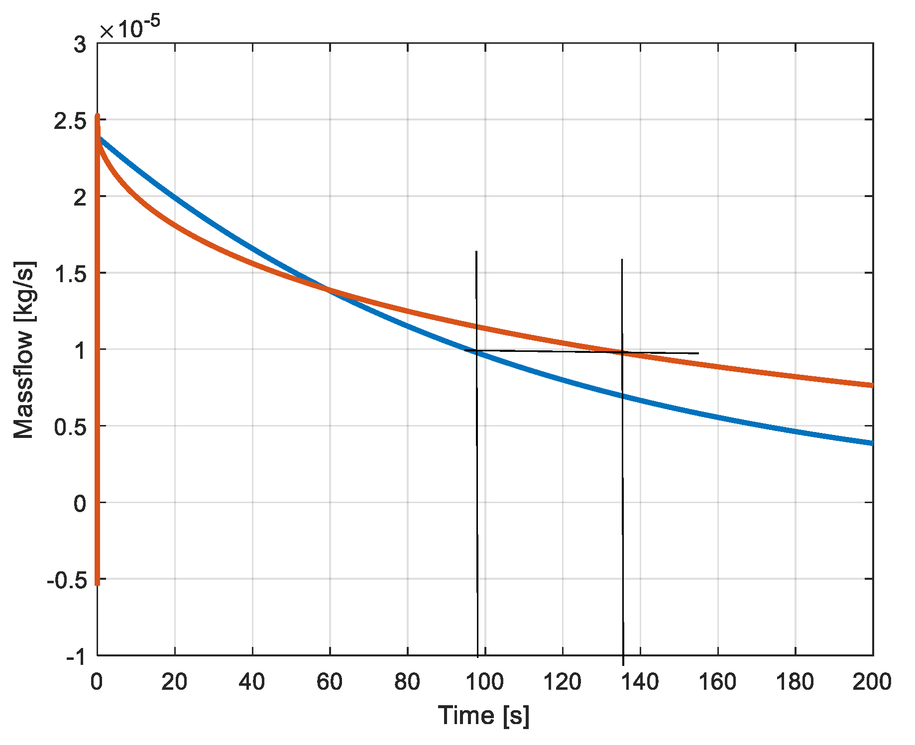
3.1. Evolution of the Pressures and Masses of Air

The evolution of the pressure in the static and dynamic reservoirs is presented in Figure 7. The blue curve shows the evolution of the pressure in the constant volume system, and the red one the pressure in the variable volume system with spring.

The evolution of the pressures is the result of the accumulated amount of air in the volumes (Figure 8) due to the injection by the compressor of the corresponding massflows (Figure 9). The blue color is again associated with the constant volume system and the red with the variable volume. The same masses of air are accumulated at the corresponding instants where the pressures are identical (254 s and 340 s).

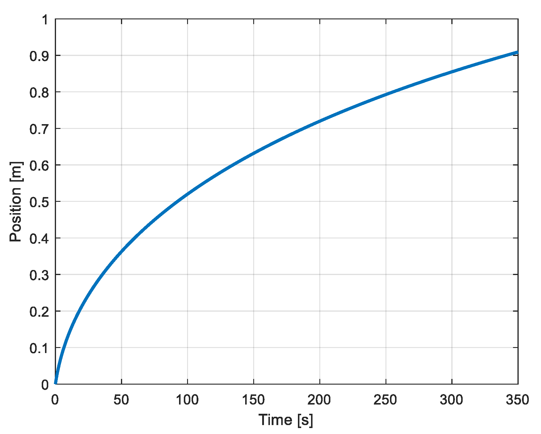
3.2. Evolution of the Mechanical Variables

In opposition to the static reservoir where only the pressure changes, the geometry of the dynamic reservoir evolves according to the change in pressure. The elevation of the pressure in the variable volume cylinder produces a directly proportional force. The evolution of the force as a function of time is represented in Figure 10. From this force, the characteristic of the spring produces a displacement of the piston, which further increases the active volume of the cylinder. The variation in the position of the piston is also directly proportional to the force, as also is the variation in the volume. The corresponding curves are given in Figure 11 and Figure 12. On these figures, one can see that the values reached at the time where the pressure is equal to 6 bar (340 s) correspond to the correct design of the system (0.9 m and 0.1 m³).

3.3. Evolution of the Energies Stored in the Systems

In the static reservoir, energy is only stored in the volume of air. Concerning the dynamic reservoir, energy is stored in the volume of compressed air and, in addition, in the loaded spring. The different values of stored energy are indicated in Figure 13. The content in the static reservoir with constant volume is indicated in blue. The value of 57,505 J (rel. (15)) is reached at the time t = 242 s. The same value is reached for the variable volume of the dynamic reservoir at the time t = 340 s (red curve). The energy stored in the spring reaches the value of 24.9 kJ at the same time magenta curve). Finally, the total amount of stored energy in the dynamic reservoir (air and spring) is represented by the yellow curve. At the full state of charge, the dynamic reservoir has accumulated the value of

$$E_{dyn}=E_{air}+E_{spring}=57.5 \mathrm{kJ}+24.9 \mathrm{kJ}=82.4 \mathrm{kJ}$$

(21)

This value represents an increase of 43% compared to the static reservoir.

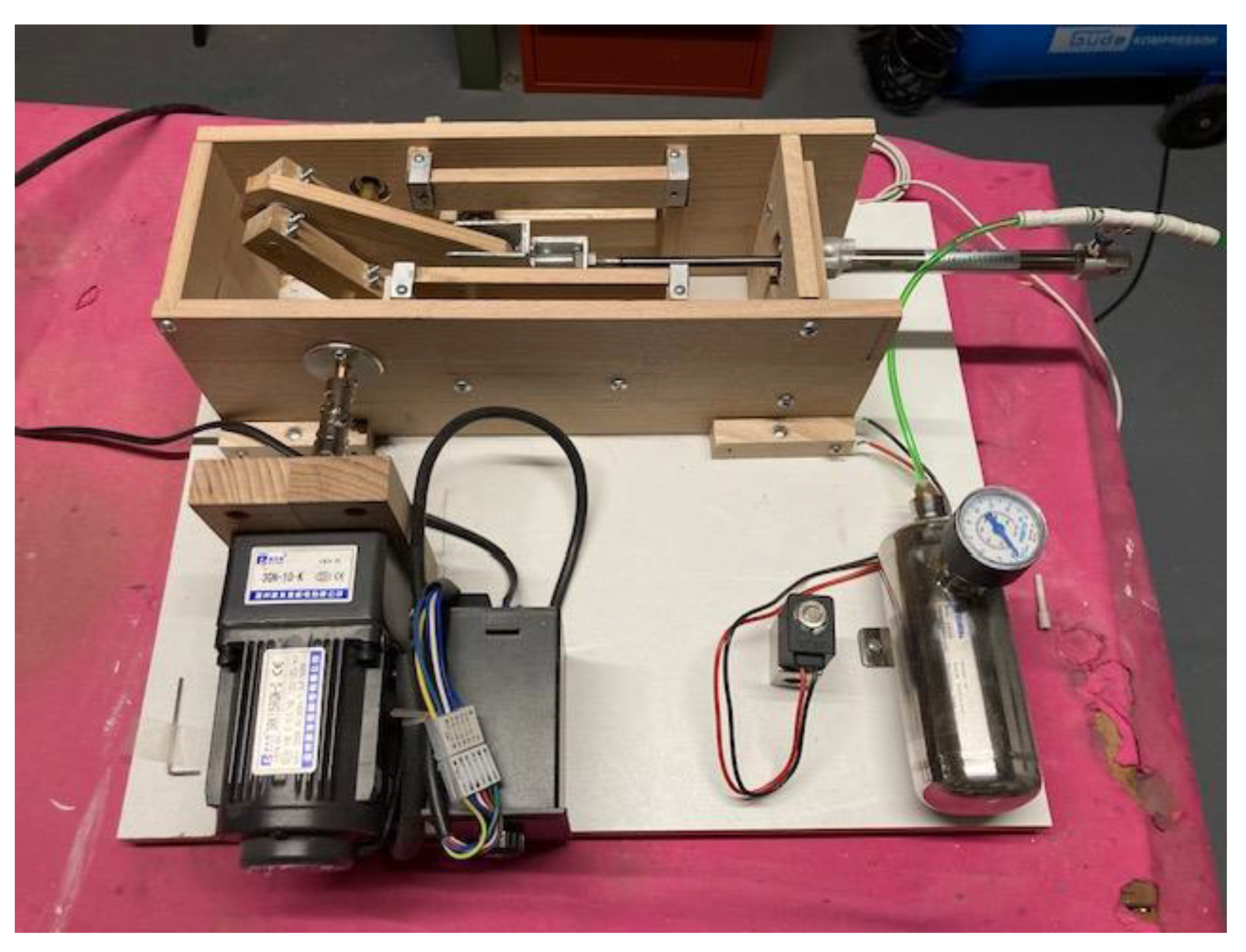
4. Analysis and Experimentation with a Small-Scale System

A small experimentation facility has been realized, comprising a compression machine and a fixed-volume reservoir. Then, the facility is completed with a reduced-scale dynamic reservoir. The compression machine is realized on the basis of a pneumatic cylinder moved with a crankshaft, itself driven by a geared variable-speed electric motor. The compression machine feeds a small reservoir of 0.3 dm³ capacity through an anti-return valve. The compression machine together with the small reservoir are represented in Figure 14.

4.1. Numeric Values of the Small Experimental Static Reservoir

The small experimentation set-up is realized with simple components available on the market and allows verification of the principles of the static and dynamic reservoirs in a simple manner. The global set of parameters is a result of using already available components at the author’s facility.

• Compression machine
• Diameter of the piston: 12 mm
• Piston stroke: 100 mm
• Volumetric ratio (Vtop/Vdown): 0.12
• Reservoir
• Volume: 0.3 L
• Rotational speed of the drive: 2 revol./s
• The volume of the cylinder of the compressor is calculated (rel. (22)):

  $$\begin{array}{l}{V}_{cyl}={\left({\displaystyle \frac{12 \mathrm{mm}}{2}}\right)}^2\cdot \pi \cdot 100 \mathrm{mm}=11309 {\mathrm{mm}}^3\\ =11309\cdot {10}^{-9} {\mathrm{m}}^3\end{array}$$

  (22)

With the value of the rotational speed, the volume flowrate becomes

$${\dot{V}}_{nom}=f\cdot {\dot{V}}_{nom}=2 {\mathrm{s}}^{-1}\cdot 11309\cdot {10}^{-9} {\mathrm{m}}^3=22.6\cdot {10}^{-6} {\mathrm{m}}^3/\mathrm{s}$$

(23)

4.2. The Small-Scale Dynamic Reservoir

The reduced scale model of the dynamic reservoir is realized with a classic pneumatic cylinder used as a variable volume. This cylinder is coupled to two parallel running springs outside of the cylinder. This configuration was chosen based on available industrial components. The parameters of the set-up components are listed in

Table 2. Parameters of the cylinder and of the spring.

Pneumatic Cylinder	SC50X175
Diameter of the piston	50 mm
Area of the piston	0.00196 m2
Maximal stroke	175 mm
Spring	T33220
De (external diameter)	50 mm
D (diameter of the spring wire)	4.5 mm
L0 (initial length)	142 mm
Ln (length under nominal load)	280 mm
Fn (nominal load)	451 N
C (spring constant)	2.77 × 103 N/m
De (external diameter)	50 mm

. The realized set-up is shown in Figure 15.

When the volume of the cylinder reaches the same value as that of the fixed reservoir (0.3 dm³), the piston has moved x_n

$$x_n={\displaystyle \frac{0.3\cdot {10}^{-3} {\mathrm{m}}^3}{0.00196 {\mathrm{m}}^2}}=0.153 \mathrm{m}$$

(24)

The two parallel running springs have the characteristics given in Table 2.

$$C_{eq}=2C=2\cdot 2.77\cdot {10}^3 \mathrm{N}/\mathrm{m}=5.54 \mathrm{kN}/\mathrm{m}$$

(25)

For a volume of 0.3 l, the force of the spring pair becomes

$$F_n=0.153m\cdot 2\cdot 2.77\cdot {10}^3 \mathrm{N}/\mathrm{m}=847.6 \mathrm{N}$$

(26)

On the rear side of the piston, the atmospheric pressure exerts a counter force of

$$F_{atm}=P_{atm}\cdot 0.00196 {\mathrm{m}}^2=196 \mathrm{N}$$

(27)

The pressure in the cylinder must generate a force able to compensate the force of the spring and of the atmosphere

$$P_n={\displaystyle \frac{847.6 \mathrm{N}+196 \mathrm{N}}{0.00196 {\mathrm{m}}^2}}=5.32\cdot {10}^5 {\mathrm{N}/\mathrm{m}}^2=5.32 \mathrm{bar}$$

(28)

As indicated in Figure 16, the variable volume of the dynamic reservoir reaches the value of 0.3 dm³ at time t = 134.7 s. At that time, the pressure in the dynamic reservoir reaches the value of 5.32 × 10⁵ N/m² (Figure 17). From the same figure, one can see that the pressure in the static reservoir reaches the same value earlier, at time t = 97 s.

4.3. Experimental Results

An experimental verification has recorded the values of the pressure in the reservoirs. They are reported on the same diagram of Figure 17. The pressure in the static reservoir is noted with (X). The pressure in the dynamic reservoir is represented in Figure 18 together with the measured values.

The pressure values indicated in Figure 17 are obtained from the calculation of the accumulated mass of air in the reservoirs. These masses are the result of the time integration of the corresponding massflows provided by the compression machine. The accumulated masses of air are represented in Figure 19, and the corresponding massflows in Figure 20.

Figure 21 shows the evolution of the piston’s position when the variable volume is filled by the compressor. The simulated value of the position reached when the pressure is 5.32 bar corresponds to the calculated value according to rel. (24). The measured positions from the set-up are also indicated in the figure (x). There is an important difference between the calculated positions and the measured ones. There was also a difference between the measured and calculated pressures (Figure 18). But the relations between measured pressures and positions correspond to the real values of the system (piston surface and spring constant). This indicates that the differences between simulated and calculated values is due to an unrealistic representation of the accumulation process of air in the reservoir. The assumption of an isothermal pressure rise in the reservoir and a nonverified value of the dead volume effect can be the main reason for the difference between simulated and measured values. The small dimensions of the experimental set-up may also have an influence.

To complete the presentation of the simulated variables, the force on the piston is represented in Figure 22.

5. Discussion

The present paper illustrates the behavior and properties of the so-called dynamic reservoir, where a mobile piston and a compression spring are integrated in the reservoir. With an accumulation volume identical to that of a classical constant-volume compressed air energy storage system, the new dynamic reservoir presents an increased energy capacity due to an accumulation of mechanical energy in the spring. The calculated benefit of capacity is around 50% (rel. (14) and (19)), and as represented in Figure 13. This value should, however, be compared with the capacity increase when a constant-volume reservoir is designed according to the real dimensions and space occupied by the compressed spring. The relation between the lengths of the deployed and compressed spring is supposed to be in a ratio of 3 to 1 (L₀ to L_N in Figure 2). As a consequence, the increased value of the volume adapted to the real dimension occupied by the spring would increase the energy capacity of a static reservoir to nearly the same value as the dynamic reservoir. The augmented static reservoir would have the advantage of a reduced number of components (no spring, no piston, no guidance rod, and no sealing joints) and would be consequently much cheaper. One advantage of the dynamic reservoir would be the benefit from pressure that is a little higher then the pressure of the static one by a low state of charge.

Cost Benefits

For the compressed air energy storage system with a design as proposed in ref. 18, namely a limited volume and a low value of pressure, it is very difficult to formulate some cost benefits due to the fact that there is a very poor energy density. The amount of stored energy in the concerned system is of around 57.5 kJ. Such an amount of energy can be stored in a Li-ion element of the size of an AA battery. The purpose of this paper was to discuss the principle of adding a spring/piston assembly, independent from the design. Further studies should analyze the same principle but with a pressure level of 100 bar. Here, the difficulty will be to design the spring to be used for additional mechanical storage.

6. Conclusions

A compressed-air energy storage system uses a traditionally pressurized reservoir, which determines the energy capacity. A new proposal recently made proposes to add inside a cylindric system a piston compressing a spring to add mechanical storage. This paper has evaluated and simulated and compared the two systems from the point of the storage capacity and the variation in the pressure based on the state of charge. The simulation has included a specific model of a compression stage where the parasitic effects like the expansion of the dead volumes on the mass flowrate are considered. The limited benefits of the added piston-spring assembly have been discussed in a specific paragraph. A further contribution to this study will be to design and simulate a dynamic reservoir system with pre-compressed spring so the pressure variation domain is reduced (starting from a higher pressure value when the piston starts to move). Such a pre-compressed spring may need a higher space in its compressed state, requiring a larger global volume. Also, a reservoir with a spring with just a higher constant would be interesting to analyze.

References

1. IPCC Intergovernmental Panel on Climate Change (IPCC) Synthesis Report. 2024. Available online: https://www.ipcc.ch/synthesis-report/ (accessed on 8 July 2025).
2. Rufer, A. Energy Storage—Systems and Components; CRC Press: Boca Raton, FL, USA, 2017. [Google Scholar]
3. Fang, R.; Zhang, R. Advances in Hybrid Energy Storage Systems and Smart Energy Grid Applications. 2021. Available online: https://www.sciencedirect.com/special-issue/10GRJ69GC0Q (accessed on 4 April 2025).
4. International Energy Agency. World Energy Outlook 2024 IEA. Available online: https://iea.blob.core.windows.net/assets/a5ba91c9-a41c-420c-b42e-1d3e9b96a215/WorldEnergyOutlook2024.pdf (accessed on 8 July 2025).
5. Adil, A.M.; Ko, Y. Socio-technical evolution of Decentralized Energy Systems: A critical review and implications for urban planning and policy. Renew. Sustain. Energy Rev. 2016, 57, 1025–1037. [Google Scholar] [CrossRef]
6. Lehmann, J. Air storage gas turbine power plants, a major distribution for energy storage. In Proceedings of the International Conference on Energy Storage, Brighton, UK, 29 April–1 May 1981; pp. 327–336. [Google Scholar]
7. The Mc Intosh CAES Power Plant, Compressed Air Energy Storage Technology: Generating Electricity Out of Thin Air. Available online: https://www.baldwinemc.com/compressed-air-energy-storage-technology-generating-electricity-out-of-thin-air/ (accessed on 22 September 2017).
8. Bradshaw, D.T. Pumped hydroelectric storage (PHS) and compressed air energy storage (CAES). In Proceedings of the 2000 Power Engineering Society Summer Meeting, Seattle, WA, USA, 16–20 July 2000; Volume 3, pp. 1551–1573. [Google Scholar]
9. Allen, K. CAES: The underground portion. IEEE Trans. Power Appar. Syst. 1985, PAS-104, 809–812. [Google Scholar] [CrossRef]
10. Ting, D.S.-K.; Stagner, J.A. Compressed Air Energy Storage: Types, Systems and Applications; The Institution of Engineering and Technology: London, UK, 2021; ISBN 978-1-83953-195-8. [Google Scholar]
11. Salvini, C.; Mariotti, P.; Giovannelli, A. Compression and Air Storage Systems for Small Size CAES Plants: Design and Off-design Analysis. Energy Procedia 2017, 107, 369–376. [Google Scholar] [CrossRef]
12. Rabi, A.M.; Radulovic, J.; Buick, J.M. Comprehensive Review of Compressed Air Energy Storage (CAES) Technologies. Thermo 2023, 3, 104–126. [Google Scholar] [CrossRef]
13. Macdonald, J. Compressed Air Energy Storage (CAES): A Comprehensive 2025 Overview. 2025. Available online: https://urbanao.com/post/compressed-air-energy-storage-caes-a-comprehensive-2025-overview (accessed on 17 June 2025).
14. Electricity Storage. Heat. Cold. Compressed Air. Combined in a Sustainable System. Available online: https://www.green-y.ch/en/ (accessed on 12 April 2025).
15. Radeska, T. The Mekarski System—Compressed-Air Propulsion System for Trams. 2016. Available online: https://www.thevintagenews.com/2016/10/17/the-mekarski-system-compressed-air-propulsion-system-for-trams/ (accessed on 28 July 2017).
16. Blain, L. AIRPod: Tiny Air-Powered Commuter Costs Half a Euro Per 100km. 2009. Available online: https://newatlas.com/airpod-compressed-air-car-mdi-zeroemissions/11177/ (accessed on 27 April 2018).
17. Lu, M.D.I. Motor Development International. 2018. Available online: https://www.mdi.lu. (accessed on 5 May 2019).
18. Kabinga, R.K.N.; Tartibu, L.K.; Okwu, M.O. Development and performance evaluation of a dynamic compressed air energy storage system. In Proceedings of the International Mechanical Engineering Congress and Exposition, Portland, OR, USA, 16–19 November 2020. [Google Scholar]
19. Cheng, Y.; Chen, K.; Chan, C.; Bouscayrol, A.; Cui, S. Global modeling and control strategy simulation. IEEE Veh. Technol. Mag. 2009, 4, 73–79. [Google Scholar] [CrossRef]
20. Shearer, M.; Gremaud, P.; Kleiner, K. Periodic motion of a mass–spring system. IMA J. Appl. Math. 2009, 74, 807–826. [Google Scholar] [CrossRef]
Figure 1. Compressed air energy storage system.
Energies 18 03666 g001
Figure 2. Static (a) and dynamic (b) compressed air reservoirs. (c) Dynamic reservoir fully loaded.
Energies 18 03666 g002
Figure 3. Effect of the expansion of the dead volume.
Energies 18 03666 g003
Figure 4. Structural diagram of the static reservoir system.
Energies 18 03666 g004
Figure 5. Schematic representation of the mass–spring system.
Energies 18 03666 g005
Figure 6. Structural diagram of the dynamic reservoir system.
Energies 18 03666 g006
Figure 7. Pressure in the reservoirs (constant volume: blue, variable volume: red).
Energies 18 03666 g007
Figure 8. Mass of air accumulated in the two reservoirs (blue: constant volume, red: variable volume).
Energies 18 03666 g008
Figure 9. Massflows to the reservoirs (blue: constant volume, red: variable volume).
Energies 18 03666 g009
Figure 10. Evolution of the force as a function of time.
Energies 18 03666 g010
Figure 11. Position of the piston.
Energies 18 03666 g011
Figure 12. Volume of the dynamic reservoir.
Energies 18 03666 g012
Figure 13. Energies accumulated in the static and dynamic reservoirs. Compressed air energy in the fixed reservoir (blue curve); compressed air energy in the variable volume (red curve); energy accumulated in the spring (magenta curve); total energy of the dynamic reservoir (yellow curve).
Energies 18 03666 g013
Figure 14. Small scale of the compression machine and of the fixed volume reservoir.
Energies 18 03666 g014
Figure 15. Reduced-scale set-up of the dynamic reservoir. (a): unloaded system, (b): system loaded at nominal pressure.
Energies 18 03666 g015
Figure 16. Volumes of the static (blue curve) and dynamic reservoir (red curve).
Energies 18 03666 g016
Figure 17. Pressures in the static (blue) and dynamic reservoir (red). The measured values of the pressure in the static reservoir are also represented (x).
Energies 18 03666 g017
Figure 18. Pressure in the dynamic reservoir -: calculated, x: measured.
Energies 18 03666 g018
Figure 19. Masses accumulated in the reservoirs (blue: static reservoir; red: dynamic reservoir).
Energies 18 03666 g019
Figure 20. Massflows provided by the compression machine (blue: static reservoir, red: dynamic reservoir).
Energies 18 03666 g020
Figure 21. Position of the piston (dynamic reservoir). The blue line corresponds to the simulated value and the measured position is represented by (x).
Energies 18 03666 g021
Figure 22. Force exerted on the piston.
Energies 18 03666 g022