Induction Motor Geometric Parameter Optimization Using a Metaheuristic Optimization Method for High-Efficiency Motor Design

Abstract

In this study, the optimum design for an induction motor (IM) was realized by providing details of its geometric design. The IM optimization was carried out using the Artificial Ecosystem-based Optimization (AEO) algorithm, a metaheuristic method. The AEO algorithm was used for the first time in IM optimization, and the design parameters were optimized. Ten motor design parameters were used as design variables. IM efficiency was improved, as the objective function. The genetic algorithm (GA) optimization method was used for comparison with the results obtained with the AEO method. The optimized and unoptimized results of the IM design generated with codes created in the Matlab program were verified with the Ansys RMxprt EM Suite 19.2 program, and it could be seen that the results are in good agreement. As a result of these studies, it was observed that the use of AEO in determining the geometric parameters of the IM had better convergence accuracy and reached the optimum result in a shorter time compared to the GA optimization method. It was observed that IM efficiency increased from 90.34% to 91.575% on average with the AEO method.

1. Introduction

In developed and developing countries, three-phase IMs still remain the preferred type of motor for use in industry. The reasons for preferring these motors are their low power consumption, durability, low maintenance, and low cost [1,2,3]. Due to their widespread use in industry, IMs constitute a large part of the total power consumption [4,5,6]. For this reason, the smallest efficiency increase in these motors provides great energy savings worldwide. In this context, the design criteria of IMs should be reviewed, higher-quality magnetic materials should be used, and the geometric parameters of the motor (rotor, stator slots, and air gap) should be determined optimally [7,8]. Geometric parameters affect motor performance in different ways. An increase in a certain parameter may increase one parameter while decreasing another [9]. Therefore, the optimization of their design is crucial for the optimal performance of IMs.

In the literature, design optimization studies to improve the performance of IMs are available and continue to be investigated [10]. The majority of these studies have generally been carried out in the form of GA optimization or derivatives of this algorithm. In [11], a numerical optimization technique was employed to minimize the effects of IM air gap harmonics and maximize the winding factor, optimizing the number of slots per pole, slot positions, and slot sizes. In [12], IM design optimization was performed using a GA, where the torque, efficiency, and cost functions were used as objective functions, resulting in a 25% reduction in motor cost. In [13], Particle Swarm Optimization (PSO) was employed to optimize the design of an IM, and the results were then compared with those obtained using a GA. The results showed a 2% increase in efficiency and an approximate increase of 2 Nm in starting torque and pull-out torque. It was concluded that successful results could be achieved in motor design using the PSO algorithm. In [14], IM design optimization was carried out using a “hybrid GA,” leading to improvements in efficiency and torque values. In [15], for electric vehicle applications, a GA was used to create a multi-objective optimization problem involving stator and rotor slot sizes to maximize the pull-out torque, efficiency, and power factor. In [16], to determine the equivalent circuit parameters of an IM, a GA and a Differential Evolution algorithm were utilized. The Differential Evolution algorithm revealed a shorter convergence time and greater precision compared to the GA. In [17], the efficiency optimization of a 3 kW IM was performed using a GA and a hybrid GA, achieving an efficiency of 86.2034% with the hybrid GA despite all constraints, which was 0.3132% higher than the efficiency obtained with the GA. In [18], it was reported that a 7.5 kW, four-pole IM was traditionally designed and then optimized using a GA in Matlab, resulting in a 1.02% increase in efficiency and a reduction of 1.11 kg in weight. In [19], the optimization of motor slot sizes using a GA resulted in an improvement in efficiency; however, altering the motor core diameters affected efficiency more significantly, with a 0.55% increase in efficiency when the stator and rotor outer diameters were increased. In [20], the optimization of losses for a 20 kVA IM was conducted using a GA, and a reduction in losses was observed through the optimization of design parameters.

This article aims to contribute to the optimization of IM design by using a new or innovative design and to obtain a more efficient design by considering the interaction of the geometric parameters of the motor. For this purpose, the aim is to reduce the losses of the IM and accordingly to obtain maximum efficiency. In order to achieve this goal, the optimization of the geometric parameters of the motor was carried out with the AEO algorithm, one of the current optimization methods, using 10 design criteria and constraints of the IM. The GA method was used to compare the optimization results obtained from the AEO algorithm, which was used for the first time in the optimization of the geometric parameters of an IM, and to evaluate the performance of the optimization algorithms. In this study, the codes of the IM design calculations and optimization algorithms were developed in the Matlab R2024a program. This study constitutes an important step that will enable more efficient and sustainable designs for electrical machines by using the AEO algorithm, which is one of the current optimization algorithms.

2. Design Calculations for Induction Motors

The IM design was carried out using the design equations from Refs. [21,22,23,24,25,26] in this section. For the IM geometry in this design, the stator geometry shown in Figure 1a and the rotor geometry shown in Figure 1b were used.

To achieve maximum efficiency, it is necessary to minimize the losses in the IM. The mathematical equations for the losses and the efficiency calculations in motor design are provided below. Stator winding losses are presented in Equation (1):

$$P_{cus}=3·R_s·I_{1n}{}^2$$

(1)

In Equation (1), $R_s$(ohm) is the stator resistance and $I_{1n}$(A) is the rated current. Rotor cage losses $P_{r1}(\mathsf{\Omega })$ are presented in Equation (2):

$$\left.\begin{array}{l}{P}_{r1}={3·(R_r)}_{sn}·K_i{}^2·I_{1n}{}^2\\ K_i=0.8·\cos \phi 1+0.2\end{array}\right\}$$

(2)

In Equation (2), ${(R_r)}_{sn}$ $(\mathrm{\Omega })$ represents the rotor resistance. The mechanical ventilation losses $P_{mv}$ (W) and stray losses $P_{stray}$ (W) are expressed by the following equations:

$$\left.\begin{array}{l}{P}_{mv}=0.012·P_n\hspace{1em}for\hspace{1em}2p=4\\ P_{stray}=0.01·P_n\end{array}\right\}$$

(3)

The stator teeth fundamental losses $P_{t1}$ (W) and stator back iron fundamental losses $P_{y1}$ (W) can be written as the following equation:

$$\left.\begin{array}{l}{P}_{t1}\cong K_t·p_{10}·{({\displaystyle \frac{F}{50}})}^{1.3}·B_{ts}{}^{1.7}·G_{t1}\\ P_{y1}\cong K_y·p_{10}·{({\displaystyle \frac{F}{50}})}^{1.3}·B_{cs}{}^{1.7}·G_{y1}\end{array}\right\}$$

(4)

In Equation (4), $p_{10}$ (W/Kg) is the specific losses at 1 Tesla and 50 Hz, the $K_t$ − $K_y$ value depends on the material quality and sharpening of the tooth, $F$ (Hz) is the frequency,$G_{t1}$ (Kg) is the stator tooth weight, $G_{y1}$ (Kg) is the stator yoke weight, $B_{ts}$ (T) is the stator tooth magnetic flux density, and $B_{cs}$ (T) is the stator yoke magnetic flux density.

$$\left.\begin{array}{l}{G}_{t1}={\gamma }_{irone}·N_s·b_{ts}·(h_{s0}+h_{s1}+h_{s2})·L·K_{FE}\\ G_{y1}={\gamma }_{irone}·{\displaystyle \frac{\pi }{4}}·\left(D_{out}{}^2-{(D_{out}-2·h_{cs})}^2\right)·L·K_{FE}\end{array}\right\}$$

(5)

In Equation (5), ${\gamma }_{irone}$ (kg/m³) is expressed as the weight of iron per unit volume, the $N_s$ value is the number of stator slots, $b_{ts}$ (m) is the stator slot teeth width, $L$ (m) is stator core length, $K_{F E}$ is the stacking factor, and $h_{cs}$ (m) is expressed as the stator yoke distance. Fundamental iron losses can be written with the following equation:

$$P_{irone1}=p_{y1}+p_{t1}$$

(6)

The tooth flux pulsation core loss $P_{irone2}$ (W) is the sum of the $p_{y1}$ and $p_{t1}$, which is given by the following equation:

$$\begin{array}{l}{P}_{irone2}=5\times {10}^{-5}\left[{\left({\displaystyle \frac{N_r·F}{p}}·{\displaystyle \frac{1}{2.2-B_{ts}}}·\left({\displaystyle \frac{tsr}{tsr-\frac{b_{r0}{}^2}{5·g-b_{r0}}}}-1\right)·B_g\right)}^2·G_{t1}+{\left({\displaystyle \frac{N_s·F}{p}}·{\displaystyle \frac{1}{2.2-B_{tr}}}·\left({\displaystyle \frac{ts}{ts-\frac{b_{s0}{}^2}{5·g-b_{s0}}}}-1\right)·B_g\right)}^2·G_{t2}\right]\\ \begin{array}{cc}& \end{array}\end{array}$$

(7)

In Equation (7), the $N_r$ value is the number of rotor slots, $tsr$(m) is the rotor slot pitch, $ts$(m) is the stator slot pitch, $B_{tr}$ (T) is the rotor tooth magnetic flux density, $g$(m) is the air gap length, and $B_g$ (T) is the air gap flux density. $G_{t2}$ represents the rotor teeth weight and is derived as follows:

$$G_{t2}={\gamma }_{irone}·N_r·(h_{r1}+{\displaystyle \frac{b_{r1}+b_{r2}}{2}})·L·K_{FE}$$

(8)

Since the output power is $P_{out}$, the efficiency of the IM can be written as follows, as in Equation (9):

$$\eta ={\displaystyle \frac{P_{out}}{P_{out}+P_{losses}}}={\displaystyle \frac{P_{out}}{P_{out}+(P_{cus}+P_{r1}+P_{mv}+P_{stray}+P_{irone1}+P_{irone2})}}$$

(9)

3. Optimization Methods Used for High-Performance IM Design

Many of the requirements for the design of an IM contradict each other. Therefore, it is very difficult to achieve a manual design that meets all the constraints. To solve this problem, computer software and optimization techniques must be used [27,28]. Optimization aims to consistently produce the best possible result [29,30]. Today, many optimization techniques have been formulated to solve the encountered problems and have been applied to various fields; the development of these techniques continues [31]. From a mathematical perspective, it is often difficult to find the most appropriate solution that meets all the objectives [32,33]. In this context, researchers have focused on developing general-purpose and high-performance optimization methods and have created optimization algorithms inspired by natural events. These methods, called metaheuristic algorithms, try to solve optimization problems by being inspired by behaviors, reactions, and communication mechanisms in nature [34,35,36,37]. Among these methods, the well-known GA method is the most widely used optimization method. In recent years, a variety of new optimization algorithms have been created; AEO is among these algorithms. These algorithms have been preferred recently due to their competitive performance in solving real engineering problems.

3.1. Genetic Algorithm

Regarding the GA, it is impossible to know the best solution at the outset. The goal is to reach the maximum or minimum point according to the objective function using algorithms. When using the GA, the problem must be accurately defined, and coding should be appropriately conducted according to the types of variables. The fitness function, which is one of the inputs to the problem, must be clearly defined. As genetic operators like crossover and mutation are used randomly during different stages of the evolutionary process, determining their application probability is important. Finally, the problem must be solved by determining the convergence criteria [38,39,40,41,42,43].

3.2. Artificial Ecosystem-Based Optimization

AEO was developed by Zhao and his colleagues in 2020. This algorithm is a population-based optimization algorithm inspired by the energy flow in an ecosystem, and this algorithm imitates three matchless behaviors of living organisms: manufacturers, consumers, and decomposers. Producers include plants that obtain the nutrients they need through photosynthesis and thus do not need to obtain energy from other organisms. They are used to increase the equilibrium between exploration and exploitation. Consumers are animals that have to obtain the energy they need from other consumer and producer groups. Animals are divided into groups such as herbivores, carnivores, and omnivores, which are both carnivores and herbivores. Decomposers are a group consisting of bacteria and fungi. This group uses the remains of dead organisms and converts them into nutrients such as water and minerals. They are proposed with the goal of improving the algorithm’s exploitation proficiency. Producers reuse these nutrients and restart the food chain cycle. The algorithm mimics this nutrient flow from producers to decomposers [44].

3.2.1. Manufacturers

The generator operator is modeled mathematically by the equation below:

$$\left.\begin{array}{l}{x}_1(t+1)=(1-\alpha )·x_n(t)+\alpha ·x_{random}(t)\\ \alpha =(1-t/t_{\max })h_1\\ x_{random}=h(U_{\mathrm{bound}}-L_{\mathrm{bound}})+L_{\mathrm{bound}}\end{array}\right\}$$

(10)

where $\alpha$ is the linear weight coefficient, n is the population size, $x_{random}$ is the location of a randomly generated individual in the search space, $t_{\max }$ is the maximum number of iterations, $h_1$ is a random number in the range [0, 1], $h$ is a random vector in the range [0, 1], and $L_{\mathrm{bound}}$ and $U_{\mathrm{bound}}$ are the lower and upper bounds, respectively.

3.2.2. Consumers

Levy is given as a consumption parameter with flight characteristics:

$$\left.D={\displaystyle \frac{1}{2}}·{\displaystyle \frac{f_1}{\left|f_2\right|}},\hspace{1em}{f}_1\sim N_{norm}(0,1),\hspace{1em}{f}_2\sim N_{norm}(0,1)\right\}$$

(11)

where $N_{norm}\left(0,1\right)$ is a normal distribution. The following equations describe three types of consumers, each randomly selected and dependent on how they interact with producers and other consumers:

• Herbivores are mathematically expressed as follows:

$$\left.x_i(t+1)=x_i(t)+D·(x_i(t)-x_1(t)),\hspace{1em}i\in [2,\dots ,n]\right\}$$

(12)

• Carnivores are mathematically formulated as follows:

$$\left.\begin{array}{l}{x}_i(t+1)=x_i(t)+D·(x_i(t)-x_j(t))\\ i\in \left[2,\dots ,n\right]\\ j=randi(\left[2i-1\right])\end{array}\right\}$$

(13)

• Omnivores are mathematically modeled as follows:

$$\left.\begin{array}{l}{x}_i(t+1)=x_i(t)+D·(x_i(t)-x_1(t))+(1-h_2)·(x_i(t)-x_j(t))\\ i=\left[3,\dots ,n\right]\\ j=randi(\left[2i-1\right])\end{array}\right\}$$

(14)

where $h_2$ is a random number in the range [0, 1].

3.2.3. Decomposition

The position of the i-th individual in the population $x_i$ can be improved to a better position depending on the discriminant $x_n$, discriminant factor E, and weight coefficients e and h, as described by the following equation:

$$\left.\begin{array}{l}{x}_i(t+1)=x_n(t)+E·(a_1·x_n(t)-a_2·x_n(t)),\hspace{1em}i=1,\dots \dots n\\ E=3·c,\hspace{1em}c\sim N(0,1)\\ a_1=h_3·randi(\left[1\hspace{1em}2\right])-1\\ a_2=2·h_3-1\end{array}\right\}$$

(15)

The AEO algorithm performs operations using Equations (10)–(15). The flow diagram of AEO is given in Figure 2.

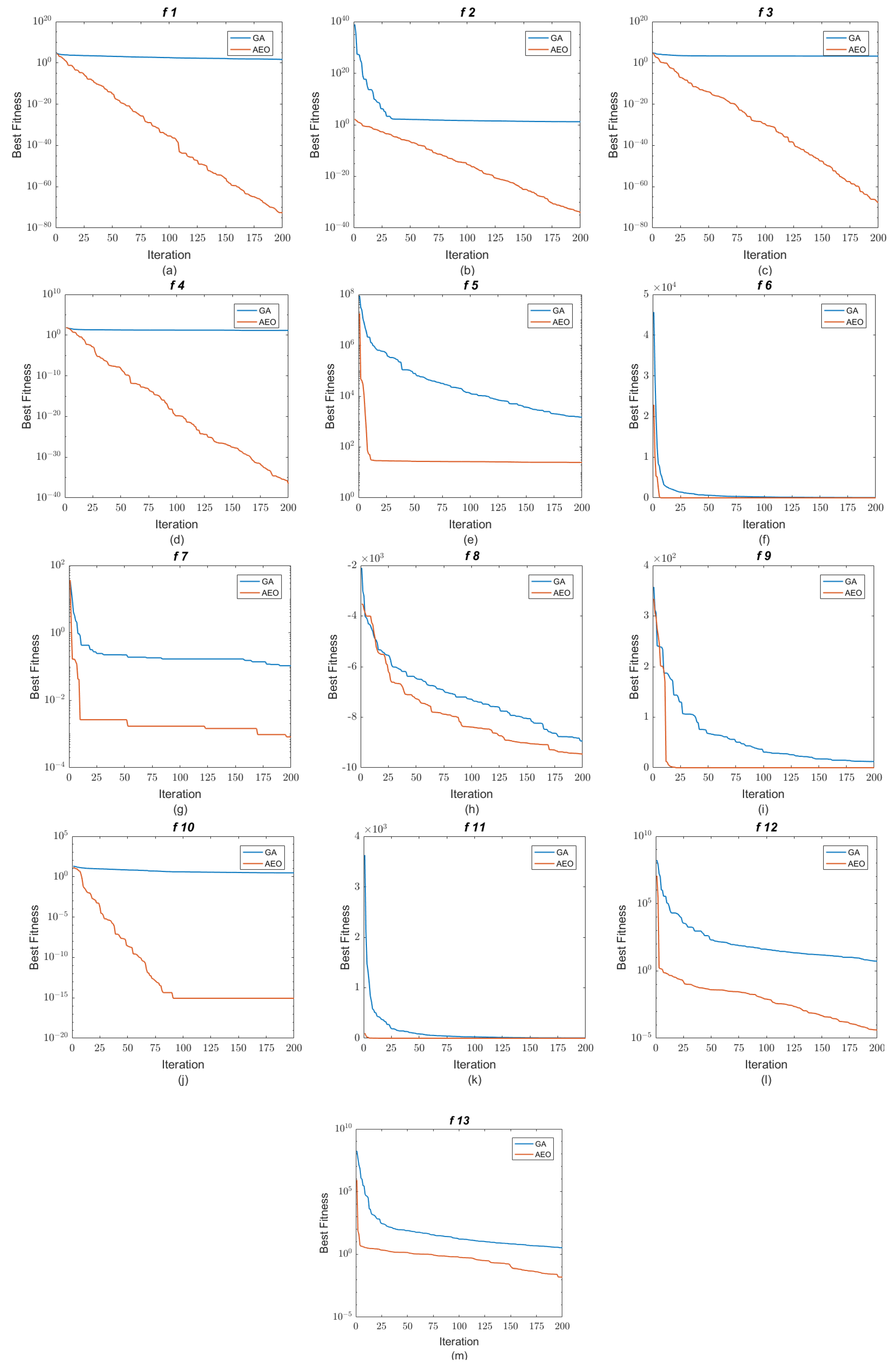
4. Comparison of AEO and GA

There are many benchmark test functions in the literature to evaluate the performance of heuristic optimization algorithms. A comprehensive analysis was performed on 13 popular benchmark test functions to evaluate the efficiency and performance of AEO and GA. The seven unimodal test functions in

Table 1. Unimodal test functions.

Function Name	Description of the Function	Dimension	Range of Values	Optimum Value
Sphere	$f_1(x)={\displaystyle {\sum }_{i=1}^n{x}_i^2}$	30	[−100, 100]	0
Schwefel 2.22	$f_2(x)={\displaystyle {\sum }_{i=1}^n\left|x_i\right|}+{\displaystyle {\prod }_{i=1}^n\left|x_i\right|}$	30	[−10, 10]	0
Schwefel 1.2	$f_3(x)={{\displaystyle {\sum }_{i=1}^n\left({\displaystyle {\sum }_{j-1}^i{x}_j}\right)}}^2$	30	[−100, 100]	0
Schwefel 2.21	$f_4(x)={\max }_i\left\{\left|x_i\right|,1\le i\le n\right\}$	30	[−100, 100]	0
Rosenbrock	$f_5(x)={\displaystyle {\sum }_{i=1}^{n-1}[100{(x_{i+1}-x_i^2)}^2+{(x_i+1)}^2]}$	30	[−30, 30]	0
Step	$f_6(x)={{\displaystyle {\sum }_{i=1}^n\left(\right[x_i+0.5\left]\right)}}^2$	30	[−100, 100]	0
Quartic	$f_7(x)={\displaystyle {\sum }_{i=1}^{n}i{x}_i^4}+random\left[0,1\right)$	30	[−1.28, 1.28]	0

have a single local minimum, while the multimodal test functions in

Table 2. Multimodal test functions.

Function Name	Description of the Function	Dimension	Range of Values	Optimum Value
Schwefel	$f_8(x)={\displaystyle {\sum }_{i=1}^n-x_i^{}}\sin \left(\sqrt{\left|x_i^{}\right|}\right)$	30	[−500, 500]	$418.9829·n$
Rastrigin	$f_9(x)={\displaystyle {\sum }_{i=1}^n[x_i^2-10\cos \left(2\pi x_i\right)+10]}$	30	[−5.12, 5.12]	0
Ackley	$f_{10}(x)=-20\exp (-0.2\sqrt{{\displaystyle \frac{1}{n}}{\displaystyle {\sum }_{i=1}^n{x}_i^2}})-\exp \left({\displaystyle \frac{1}{n}}{\displaystyle {\sum }_{i=1}^n\cos (2\pi x_i)}\right)+20+e$	30	[−32, 32]	0
Griewank	$f_{11}(x)={\displaystyle \frac{1}{400}}{\displaystyle {\sum }_{i=1}^n{x}_i^2}-{\displaystyle {\prod }_{i=1}^n\cos (\frac{x_i}{\sqrt{i}}})+1$	30	[−600, 600]	0
Penalized	$\begin{array}{l}{f}_{12}(x)={\displaystyle \frac{\pi }{n}}\left\{\left(10\sin (\pi y_1)\right)+{{\displaystyle {\sum }_{i=1}^{n-1}\left(y_1-1\right)}}^2\left[1+10{\sin }^2(\pi y_{i+1})\right]+{\left(y_n-1\right)}^2\right\}+\pi \\ {\displaystyle {\sum }_{i=1}^{n}u(x_1,10,100.4)}\\ y_i=1+{\displaystyle \frac{x_i+1}{4}}\\ u\left(x_i,a,k,m\right)=\left\{\begin{array}{c}k(x_i-a)\hspace{1em}{x}_i>a\\ 0-a<x_i<a\\ k{(-x_i-a)}^m\hspace{1em}{x}_i<-a\end{array}\right\}\end{array}$	30	[−50, 50]	0
Penalized 2	$\begin{array}{l}{f}_{13}(x)=0.1\left\{{\sin }^2(3\pi x_1\right.)+{{\displaystyle {\sum }_{i=1}^n\left(x_i-1\right)}}^2\left[1+{\sin }^2(3\pi x_i+1)\right]+\\ \left.{(x_n-1)}^2\left[1+{\sin }^2(2\pi x_n)\right]\right\}+{\displaystyle {\sum }_{i=1}^{n}u(x_i,5,100,4)}\end{array}$	30	[−50, 50]	0

have multiple local minimums [45]. The chosen test functions are effective in assessing the convergence behavior of the algorithms.

Two optimization algorithms were applied to 13 test functions, 7 of which were unimodal and 6 of which were multimodal. Each algorithm was run 10 times for each function. To ensure a fair comparison, the population size for each algorithm was set to 50, and the maximum number of iterations was set to 200. The statistical results for these 13 test functions are presented in

Table 3. Comparison of optimization results for various test functions.

Function Number	Index	Optimization Techniques
		GA	AEO
$f_1(x)$	Average	22.4545	4.5414 × 10−66
	Standard Deviation	5.7000	1.0185 × 10−65
	Best Value	12.9998	6.7211 × 10−78
$f_2(x)$	Average	0.8488	1.8175 × 10−32
	Standard Deviation	0.1796	5.0184 × 10−32
	Best Value	0.5578	2.5352 × 10−38
$f_3(x)$	Average	2.895 × 103	2.8105 × 10−68
	Standard Deviation	8.131 × 102	6.9181 × 10−68
	Best Value	1.926 × 103	2.1721 × 10−78
$f_4(x)$	Average	6.176	4.1896 × 10−32
	Standard Deviation	1.182	1.0889 × 10−31
	Best Value	4.941	2.6871 × 10−35
$f_5(x)$	Average	3.905 × 102	2.5105 × 101
	Standard Deviation	1.602 × 102	7.2142 × 101
	Best Value	2.146 × 102	2.4201 × 101
$f_6(x)$	Average	10.16	0
	Standard Deviation	1.532	0
	Best Value	8.526	0
$f_7(x)$	Average	4.714 × 10−2	1.3587 × 10−3
	Standard Deviation	1.124 × 10−2	1.4657 × 10−3
	Best Value	3.173 × 10−2	1.4071 × 10−4
$f_8(x)$	Average	−9.462 × 103	−9.7426 × 103
	Standard Deviation	3.380 × 102	5.3122 × 102
	Best Value	−9.918 × 103	−1.0820 × 104
$f_9(x)$	Average	18.950	0
	Standard Deviation	4.540	0
	Best Value	11.69	0
$f_{10}(x)$	Average	1.462	8.8818 × 10−12
	Standard Deviation	5.466 × 10−1	1.7030 × 10−27
	Best Value	7.713 × 10−3	8.8818 × 10−12
$f_{11}(x)$	Average	1.065	0
	Standard Deviation	3.147 × 10−2	0
	Best Value	1.011	0
$f_{12}(x)$	Average	2.060 × 10−1	3.7326 × 10−5
	Standard Deviation	2.078 × 10−1	2.1774 × 10−5
	Best Value	1.680 × 10−2	1.3847 × 10−5
$f_{13}(x)$	Average	7.227 × 10−1	0.1069
	Standard Deviation	1.705 × 10−1	0.1300
	Best Value	4.549 × 10−1	6.6828 × 10−3

.

It is seen that the AEO algorithm has the best average solution, minimum convergence, and standard deviation value in the unimodal and multimodal test functions. The performance curves of the GA and AEO optimization algorithms in the 13 quality test functions are given in more detail in Figure 3.

When the performance curves of the two algorithms given in Figure 3 are examined, it is seen that the AEO algorithm converges better than the GAs. Especially for the functions f5, f6, and f11, the AEO algorithm converges in small iterations at the 20th iteration. In general, the AEO algorithm shows excellent convergence ability and superior performance in most of the comparison functions.

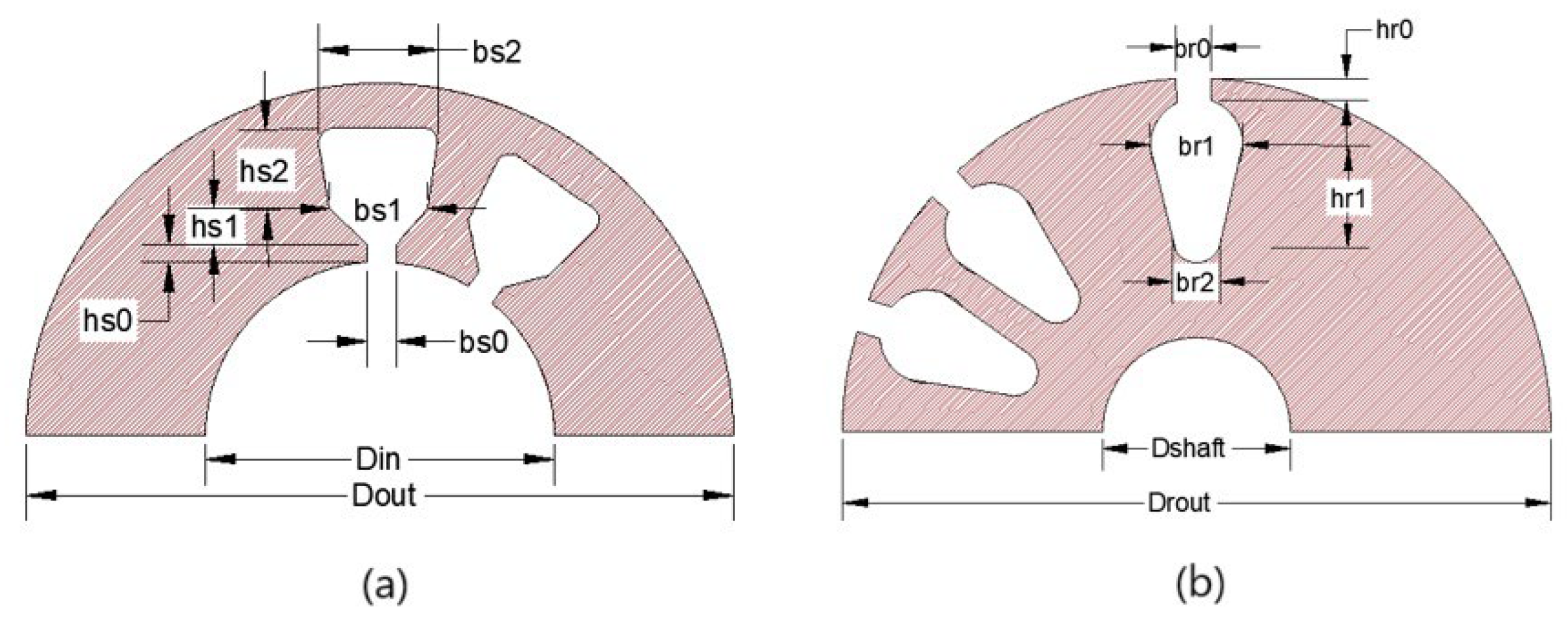
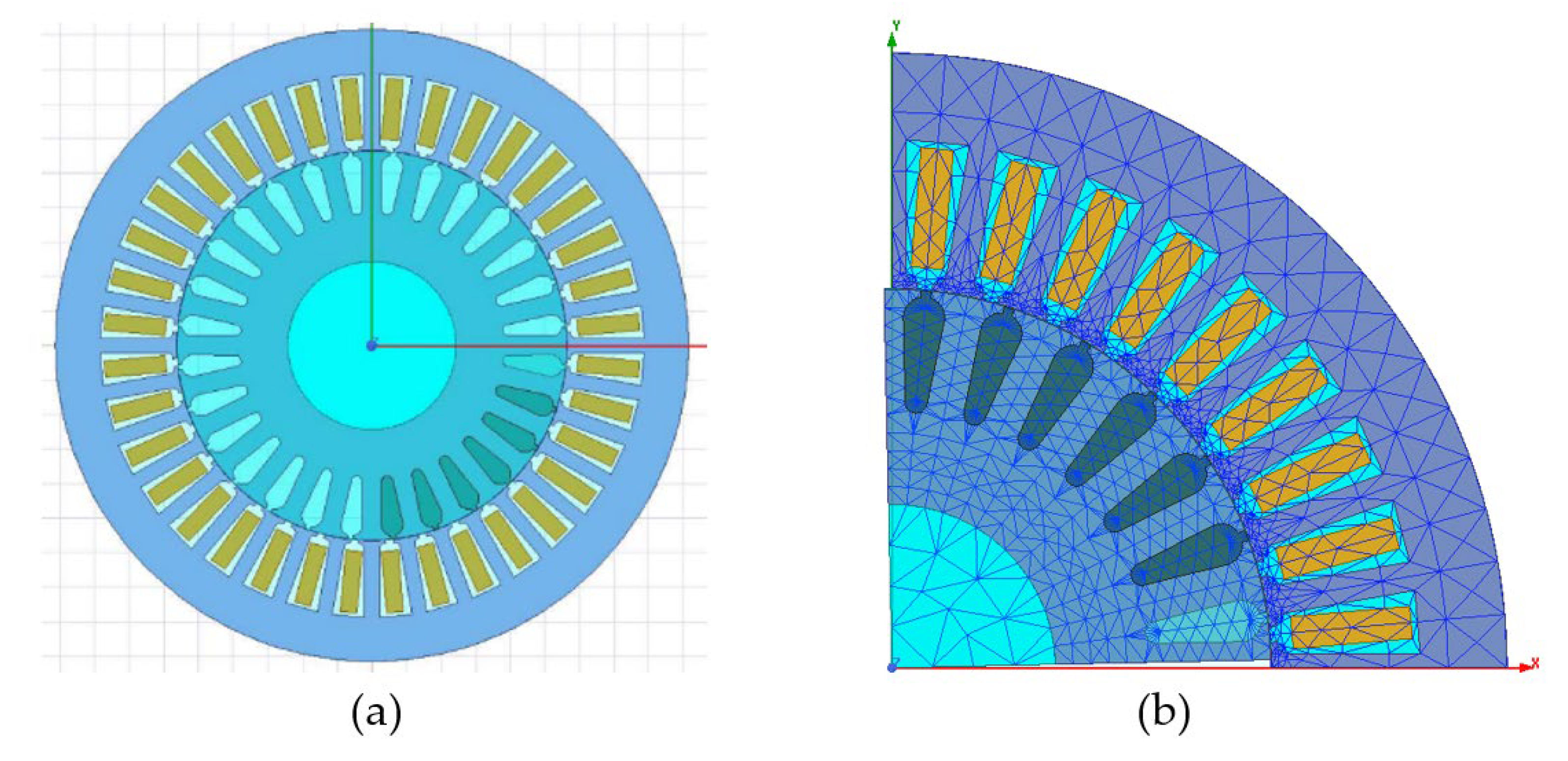
5. Design Procedure for an Induction Motor

In the IM optimization study, it is very important to determine the objective function and the relevant motor parameters, to determine the limits of the determined motor parameters, and to determine the constraints. The IM parameters used in this study are presented in Table 4.

Table 4. IM specifications used in this study [21].

Description/Symbols	Units	Values	Description/Symbols	Units	Values
$(Pout)$	kW	5.5	$(bs0)$	mm	2.2
$\mathrm{Applied} \mathrm{voltage}-(Vin)$	Volt	460	$(hs0)$	mm	1
$(F)$	Hz	60	$(hs1)$	mm	1.5
$\mathrm{Number} \mathrm{of} \mathrm{phases}-(m)$		3	$(N_r)\hspace{0.17em}$		28
$\mathrm{Number} \mathrm{of} \mathrm{poles}-(2p)$		4	$\mathrm{Rotor} \mathrm{bars} \mathrm{per} \mathrm{slot}-(Z_{sr})\hspace{0.17em}$		1
$(\eta )$		0.895	$\mathrm{Rotor} \mathrm{current} \mathrm{density}-(J_b)$	$\mathrm{A}/\mathrm{m}{\mathrm{m}}^2$	3.42
$\mathrm{Targeted} \mathrm{power} \mathrm{factor}-(\cos \phi )$		0.83	$\mathrm{Flux} \mathrm{density} \mathrm{of} \mathrm{rotor} \mathrm{tooth}-(B_{tr})$	T	1.60
$(N_s)\hspace{0.17em}$		36	$\mathrm{Flux} \mathrm{density} \mathrm{of} \mathrm{rotor} \mathrm{backcore}-(B_{cr})$	T	1.60
$\mathrm{Stator} \mathrm{current} \mathrm{density}-(J_{stator})$	$\mathrm{A}/\mathrm{m}{\mathrm{m}}^2$	4.50	$\mathrm{Current} \mathrm{density} \mathrm{of} \mathrm{endrings}-(J_{er})$	$\mathrm{A}/\mathrm{m}{\mathrm{m}}^2$	0.75 × $J_b$
$(B_g)$	T	0.70	$(br0)$	mm	1.5
$(B_{ts})$	T	1.55	$(hr0)$	mm	1
$(K_{FE})$		0.95	$\mathrm{Copper} \mathrm{resistivity} \mathrm{at} 20°\mathrm{C}-({({\rho }_{co})}_{{20}^o C})$	$\mathsf{\Omega }\mathrm{m}$	1.78 × 10−8
$({\gamma }_{irone})$	$\mathrm{kg}/{\mathrm{m}}^3$	7800	$\mathrm{Copper} \mathrm{resistivity} \mathrm{at} 80 °\mathrm{C}-({({\rho }_{co})}_{{80}^o C})$	$\mathsf{\Omega }\mathrm{m}$	2.17 × 10−8
			$\mathrm{Resistivity} \mathrm{of} \mathrm{aluminum} \mathrm{at} 20 °\mathrm{C}-({({\rho }_{AL})}_{{20}^o C})$	$\mathsf{\Omega }\mathrm{m}$	3.1 × 10−8

Table 4. IM specifications used in this study [21].

Description/Symbols	Units	Values	Description/Symbols	Units	Values
$(Pout)$	kW	5.5	$(bs0)$	mm	2.2
$\mathrm{Applied} \mathrm{voltage}-(Vin)$	Volt	460	$(hs0)$	mm	1
$(F)$	Hz	60	$(hs1)$	mm	1.5
$\mathrm{Number} \mathrm{of} \mathrm{phases}-(m)$		3	$(N_r)\hspace{0.17em}$		28
$\mathrm{Number} \mathrm{of} \mathrm{poles}-(2p)$		4	$\mathrm{Rotor} \mathrm{bars} \mathrm{per} \mathrm{slot}-(Z_{sr})\hspace{0.17em}$		1
$(\eta )$		0.895	$\mathrm{Rotor} \mathrm{current} \mathrm{density}-(J_b)$	$\mathrm{A}/\mathrm{m}{\mathrm{m}}^2$	3.42
$\mathrm{Targeted} \mathrm{power} \mathrm{factor}-(\cos \phi )$		0.83	$\mathrm{Flux} \mathrm{density} \mathrm{of} \mathrm{rotor} \mathrm{tooth}-(B_{tr})$	T	1.60
$(N_s)\hspace{0.17em}$		36	$\mathrm{Flux} \mathrm{density} \mathrm{of} \mathrm{rotor} \mathrm{backcore}-(B_{cr})$	T	1.60
$\mathrm{Stator} \mathrm{current} \mathrm{density}-(J_{stator})$	$\mathrm{A}/\mathrm{m}{\mathrm{m}}^2$	4.50	$\mathrm{Current} \mathrm{density} \mathrm{of} \mathrm{endrings}-(J_{er})$	$\mathrm{A}/\mathrm{m}{\mathrm{m}}^2$	0.75 × $J_b$
$(B_g)$	T	0.70	$(br0)$	mm	1.5
$(B_{ts})$	T	1.55	$(hr0)$	mm	1
$(K_{FE})$		0.95	$\mathrm{Copper} \mathrm{resistivity} \mathrm{at} 20°\mathrm{C}-({({\rho }_{co})}_{{20}^o C})$	$\mathsf{\Omega }\mathrm{m}$	1.78 × 10−8
$({\gamma }_{irone})$	$\mathrm{kg}/{\mathrm{m}}^3$	7800	$\mathrm{Copper} \mathrm{resistivity} \mathrm{at} 80 °\mathrm{C}-({({\rho }_{co})}_{{80}^o C})$	$\mathsf{\Omega }\mathrm{m}$	2.17 × 10−8
			$\mathrm{Resistivity} \mathrm{of} \mathrm{aluminum} \mathrm{at} 20 °\mathrm{C}-({({\rho }_{AL})}_{{20}^o C})$	$\mathsf{\Omega }\mathrm{m}$	3.1 × 10−8

The IM analytical calculations are explained in detail in Section II. Analytical calculations of the motor were performed with codes created in the Matlab program. Geometric dimensions of the pre-designed motor were obtained. The geometric dimensions of the motor obtained as a result of analytical calculations are presented in

Table 5. Geometric dimensions of the IM obtained as a result of the preliminary design in the Matlab program.

Description/Symbols	Units	Values	Description/Symbols	Units	Values
$Dout$	mm	182.9	$br0$	mm	1.5
$Din$	mm	112.9	$br1$	mm	6.2
$L$	mm	133	$br2$	mm	3.3
$g$	mm	0.31	$hr0$	mm	1
$bs0$	mm	2.2	$hr1$	mm	12.6
$bs1$	mm	6	$Dshaft$	mm	48.6
$bs2$	mm	9.4
$hs0$	mm	1
$hs1$	mm	1.5
$hs2$	mm	19.5

.

Using the motor’s geometric dimensions obtained from Table 5, the analysis of the IM was recalculated with a program that performs analytical calculations based on the motor’s geometric dimensions, which were created in the Matlab program. The results of the IM’s analytical calculations are presented in

Table 6. Motor analysis results calculated in the Matlab program and analysis results obtained in the Ansys RMxprt program.

Motor Parameter Name—Units	Matlab Program Calculation Results	Ansys-RMxprt Calculation Results
Specific Electric Loading—Am	26,789	26,776
Rated Current—A	9.1059	9.097
Magnetization Current—A	4.2578	4.250
Rotor Current—A	8.0491	7.663
Air Gap Flux Density—T	0.6915	0.6918
Stator Teeth Flux Density—T	1.6714	1.6675
Rotor Teeth Flux Density—T	1.6740	1.6542
Stator Yoke Flux Density—T	1.7841	1.8178
Rotor Yoke Flux Density—T	1.7194	1.6379
Air Gap mmf—Aturns	104.6079	120.903
Stator Tooth mmf—Aturns	88.4325	80.875
Rotor Tooth mmf—Aturns	40.23	58.6951
Stator Yoke mmf—Aturns	246.2024	168.834
Rotor Yoke mmf—Aturns	69.6702	20.0847
Stator Phase Resistance—ohm	0.8273	0.9111
Rotor Resistance—ohm	0.8990	0.7915
Stator Phase Leakage Reactance—ohm	2.2966	2.009
Rotor Leakage Reactance—ohm	3.1794	2.1362
Magnetization Reactance—ohm	58.7326	58.52
Stator Core Steel Weigh—kg	10.1873	10.3368
Rotor Core Steel Weight—kg	5.2155	5.7586
Stator Ohmic Loss—W	205.5864	226.205
Rotor Ohmic Loss—W	173.5334	139.481
Iron Core Losses—W	86.8155	80.930
Frictional and Windage Loss—W	66	66.336
Stray Loss—W	55	55
Output Power—W	5491.1	5500.33
Efficiency—%	90.34	90.64
Power Factor	0.8517	0.8296
Rated Torque—Nm	30.087	29.9113
Rated Slip	0.0302	0.0244

. To assess the accuracy of the results, the IM analysis was also conducted using the Ansys RMxprt program, employing the same geometric measurements. The motor analysis results obtained from the Ansys RMxprt program are also provided in the table for comparison.

For the design optimization of the IM, 10 of the geometric dimensions of the motor were selected as design parameters. The selected parameters, along with their initial values and upper and lower bounds are presented in

Table 7. Design parameters and boundary values used in IM design.

Description	Units	Lower	Real Values	Upper
$ns(x1)$		25	29	35
$D_{in}(x2)$	mm	100	112.9	120
$L(x3)$	mm	120	133	150
$h_{s0}(x4)$	mm	0.3	1	1.2
$h_{s1}(x5)$	mm	1	1.5	2
$h_{s2}(x6)$	mm	19	19.5	22
$b_{s0}(x7)$	mm	2	2.2	3
$b_{s1}(x8)$	mm	5	6	7
$b_{s2}(x9)$	mm	8	9.4	12
$D_{out}(x10)$	mm	175	1829	210

. During the optimization study, a constraint of two decimal places was applied to determine the motor parameters, and the number of conductors per slot $ns$ was treated as an integer in the code.

Constraints play an essential role in the manufacturing of a motor, and a motor should be manufactured by paying attention to the specified constraints. These constraints can directly affect the performance and reliability of the motor. In addition, the constraints shape the success of the optimization process by affecting the change in the objective function. Therefore, all constraints used in the design process should be carefully selected and applied. The constraints considered during the design are presented in

Table 8. Constraints used in the IM design procedure.

Description	Units	Design Parameter Name	Limit
$B_g(Y1)$	T		$\le$0.75
$K_{fill}(Y2)$			$\le$0.6
$B_{cs}(Y3)$	T		$\le$1.7
$B_{cr}(Y4)$	T		$\le$1.7
$B_{ts}(Y5)$	T		$\le$1.7
$\cos \phi (Y6)$			$\ge$0.80
$t_{LR}(Y7)$		$\mathrm{Starting} \mathrm{torque} / \mathrm{Rated} \mathrm{torque}$	$\ge$1.2
$t_{bk}(Y8)$		$\mathrm{Breakdown} \mathrm{torque} / \mathrm{Rated} \mathrm{torque}$	$\ge$1.75
$i_{LR}(Y9)$		$\mathrm{Locked} \mathrm{rotor} \mathrm{current} / \mathrm{Rated} \mathrm{current}$	$\le$7

.

6. Results and Discussion

In developing the proposed algorithms, a computer with an Intel Core i3-1115G4 CPU running at 3 GHz with 8 GB of RAM and a 256 GB SSD was used to ensure efficient and fast algorithm performance. The algorithms and calculations were performed in the Matlab program. The GA and AEO optimization algorithms were run based on the 10 design parameters given in Table 7 and the 9 constraints given in Table 8. As the objective function, the IM efficiency value expressed in Equation (9) was improved. The two optimization algorithms were set to 50 iterations and run twenty times. The objective function values and solution times of the algorithms were examined by taking the average of the objective function values and solution times obtained as a result of both optimizations. These values are listed in

Table 9. Average of the objective function and solution time values of the GA and AEO optimization algorithms for IM design optimization.

Description	GA		AEO
	CPU Time (s)	(η)%	CPU Time (s)	(η)%
Average	111.211	91.382	52.84	91.575
Standard Deviation		0.1192		0.08720

.

When the average values presented in Table 9 are examined, it is seen that the algorithm that reaches the solution the fastest is the AEO algorithm. Both algorithms provide a significant improvement in terms of optimum solutions compared to the motor efficiency of the initial motor design. The design parameters of the IM and the solution times of the algorithms for results close to the average efficiency values obtained by running the optimization methods twenty times are presented in

Table 10. The design parameters of the IM that give the result closest to the average efficiency values obtained by running the optimization algorithms twenty times.

Description	Units	M1	Design Parameter Values
			M2	M3
$ns(x1)$		29	27	26
$D_{in}(x2)$	mm	112.9	115.75	118.69
$L(x3)$	mm	133	138.84	142.59
$h_{s0}(x4)$	mm	1	0.61	0.51
$h_{s1}(x5)$	mm	1.5	1.3	1.46
$h_{s2}(x6)$	mm	19.5	20.82	19.97
$b_{s0}(x7)$	mm	2.2	2.2	2.3
$b_{s1}(x8)$	mm	6	5.51	6.36
$b_{s2}(x9)$	mm	9.4	9.66	8.23
$D_{out}(x10)$	mm	182.9	204.63	198.42
$\eta$ (Ansys RMxprt)	%	90.64	91.87	91.97
$\eta$ (Matlab)	%	90.34	91.45	91.61
Optimization running time in the Matlab program	sec		106.5485	52.1754
Change in efficiency of the M2 and M3 motor designs compared to the M1 motor design	%		1.22	1.4

. In Table 10, the motor designed with the design parameters obtained as a result of the first design is expressed as M1, the motor designed with the design parameters obtained with the GA is expressed as M2, and the motor designed with the design parameters obtained with the AEO algorithm is expressed as M3. In addition, the efficiency values obtained as a result of the analytical calculations performed in the Ansys RMxprt program according to the optimum design parameters are given in Table 10.

The average efficiency values obtained by running the GA and AEO optimization algorithms twenty times on the IM design increased to 91.382% and 91.575%, respectively, while the initial efficiency value was 90.34%. Table 10 presents the IM design parameters for results close to the average efficiency values of the algorithms. When Table 10 is examined, the M3 motor design has better results than the M2 motor design. This shows that the IM design obtained with the AEO algorithm has an advantage over the design obtained with the GA. In addition, the AEO algorithm showed the best performance in terms of solution time. This advantage in solution time will provide great advantages in terms of saving time and obtaining faster results in applications with a large number of variables.

The motors designed and the motor models obtained from the optimization results were examined using Finite Element Analysis (FEA) for electromagnetic field analysis in the Ansys RMXprt program. The motor models were created in two dimensions, as shown in Figure 4a, and the mesh pattern for a quarter part of the IM was created, as shown in Figure 4b.

In the 2D analysis, in order to reduce the simulation time, the analysis was performed on a quarter of the IM. The analysis was carried out for the entire motor, and the magnetic flux density was shown on the quarter section of the motor.

When Figure 4b is examined, the analysis is more precise in areas with a dense mesh pattern. In the 2D analysis, the simulation results were obtained with an analysis performed over a 0.2 s interval, at a precision of 0.0005 s. Figure 5 shows the distribution of magnetic flux density for all three motor designs.

When the distributions obtained as a result of the solution are examined, it is seen that the average flux density values are within the limits. The results obtained from the Ansys program at this stage show that the models were created correctly. The correct magnetic flux densities also ensured that the performance characteristics of the IM were obtained correctly.

The efficiency of the designed motor has been significantly increased by optimizing the design of geometric dimensions such as the stator slot, inner diameter, outer diameter, and core length. This is an effective method to improve the overall performance and energy efficiency of the motor. However, the limitations in the physical structure of the motor, especially the limited space in the motor body, can make it difficult to apply such optimizations to every motor. In other words, it may not be possible to implement such improvements in every design because certain motor designs may not be able to accept these changes due to space constraints and other structural factors. On the other hand, iron core losses are an important factor that negatively affects the efficiency of motors. These losses are usually caused by heat generation caused by magnetic flux changes inside the motor. When core losses increase, the operating temperature of the motor increases, which can limit the load carrying capacity of the motor. To overcome this problem, a suitable higher-quality magnetic material selection improves the performance of the motor, both increasing efficiency and helping to keep the temperature levels of the motor under control. Reducing rotor copper losses is another important factor that increases the efficiency of the motor. Although traditionally cast aluminum material is widely used in rotor manufacturing, the electrical conductivity of aluminum is lower than copper. Therefore, the use of copper material significantly reduces the electrical losses on the rotor, increasing the motor efficiency.

As a result, motor efficiency can be increased by a combination of factors such as stator–rotor material and design optimizations. However, it should be noted that these optimizations must be performed carefully, considering the physical limitations of the motor and the design requirements.

7. Conclusions

In this study, motor design optimization is explored using the current optimization algorithm, AEO, to idealize the parameters of an IM. The optimal design parameters are determined by maximizing motor efficiency as the objective function. The design optimization considers all relevant motor parameters and constraints. In order to highlight the potential of the AEO method, which was used for the first time in IM design optimization, this method is compared with the GA, which has been extensively utilized in this field. The results, based on the average values from running the optimization algorithms twenty times, show a 1.36% increase in motor efficiency using AEO and a 1.15% increase using the GA compared to the initial efficiency. Additionally, the average solution times for the methods are 52.84 s for AEO and 111.21 s for the GA, demonstrating that AEO provides faster solution times than the GA. Overall, the AEO algorithm proves to be more effective than the GA in optimizing the design to maximize efficiency in IMs. It is anticipated that this study will contribute to future research. Optimization studies will be conducted using different stator slot geometries, and the most optimal slot structure will be determined.

References

1. Renier, B.; Hameyer, K.; Belmans, R. Comparison of standards for determining efficiency of three phase induction motors. IEEE Trans. Energy Convers. 1999, 14, 512–517. [Google Scholar] [CrossRef]
2. Zhou, P.; Xu, Y.; Zhang, W. Design Consideration on a Low-Cost Permanent Magnetization Remanufacturing Method for Low-Efficiency Induction Motors. Energies 2023, 16, 6142. [Google Scholar] [CrossRef]
3. Mahmouditabar, F.; Baker, N.J. Design Optimization of Induction Motors with Different Stator Slot Rotor Bar Combinations Considering Drive Cycle. Energies 2024, 17, 154. [Google Scholar] [CrossRef]
4. Gangsar, P.; Tiwari, R. Signal based condition monitoring techniques for fault detection and diagnosis of induction motors: A state-of-the-art review. Mech. Syst. Signal Process. 2020, 144, 106908. [Google Scholar] [CrossRef]
5. Saidur, R. A review on electrical motors energy use and energy savings. Renew. Sustain. Energy Rev. 2010, 14, 877–898. [Google Scholar] [CrossRef]
6. Ghosh, P.K.; Sadhu, P.K.; Basak, R.; Sanyal, A. Energy efficient design of three phase induction motor by water cycle algorithm. Ain Shams Eng. J. 2020, 11, 1139–1147. [Google Scholar] [CrossRef]
7. Verucchi, C.; Ruschetti, C.; Giraldo, E.; Bossio, G.; Bossio, J. Efficiency optimization in small induction motors using magnetic slot wedges. Electr. Power Syst. Res. 2017, 152, 1–8. [Google Scholar] [CrossRef]
8. Danin, Z.; Sharma, A.; Averbukh, M.; Meher, A. Improved Moth Flame Optimization Approach for Parameter Estimation of Induction Motor. Energies 2022, 15, 8834. [Google Scholar] [CrossRef]
9. Sun, Z.; Hu, J.; Xin, Y.; Guo, Q.; Yao, Z. Multi-objective structure optimization for interior permanent magnet synchronous motors under complex operating conditions. Struct. Multidiscip. Optim. 2024, 67, 120. [Google Scholar] [CrossRef]
10. Mallik, S.; Mallik, K.; Barman, A.; Maiti, D.; Biswas, S.K.; Deb, N.K.; Basu, S. Efficiency and cost optimized design of an induction motor using genetic algorithm. IEEE Trans. Ind. Electron. 2017, 64, 9854–9863. [Google Scholar] [CrossRef]
11. Gulbahce, M.O.; Kocabas, D.A. High-speed solid rotor induction motor design with improved efficiency and decreased harmonic effect. IET Electr. Power Appl. 2018, 12, 1126–1133. [Google Scholar] [CrossRef]
12. Çunkaş, M.; Akkaya, R. Design optimization of induction motor by genetic algorithm and comparison with existing motor. Math. Comput. Appl. 2006, 11, 193–203. [Google Scholar] [CrossRef]
13. Chekroun, S.; Abdelhadi, B.; Benoudjit, A. A New approach design optimizer of induction motor using particle swarm algorithm. AMSE J. Ser. Model. A 2014, 87, 89–108. [Google Scholar]
14. Chekroun, S.; Abdelhadi, B.; Benoudjit, A. Design optimization of induction motor using hybrid genetic algorithm «a critical analyze». AMSE J. Ser. Adv. C 2015, 71, 1–23. [Google Scholar]
15. Akhtar, M.J.; Behera, R.K. Optimal design of stator and rotor slot of induction motor for electric vehicle applications. IET Electr. Syst. Transp. 2019, 9, 35–43. [Google Scholar] [CrossRef]
16. Arslan, M.; Çunkaş, M.; Sağ, T. Determination of induction motor parameters with differential evolution algorithm. Neural Comput. Appl. 2012, 21, 1995–2004. [Google Scholar] [CrossRef]
17. Tai, Y.; Liu, Z.; Yu, H.; Liu, J. Efficiency optimization of induction motors using genetic algorithm and Hybrid Genetic Algorithm. In Proceedings of the 2011 International Conference on Electrical Machines and Systems, Beijing, China, 20–23 August 2011; pp. 1–4. [Google Scholar] [CrossRef]
18. Gupta, A.; Machavaram, R.; Kshatriya, T.; Ranjan, S. Multi-objective design optimization of a three phase squirrel cage induction motor for electric propulsion system using genetic algorithm. In Proceedings of the 2020 IEEE First International Conference on Smart Technologies for Power, Energy and Control (STPEC), Nagpur, India, 25–26 September 2020; pp. 1–6. [Google Scholar]
19. Nakhaei, M.R.; Roshanfekr, R. Optimal Design of 3-phase Squirrel Cage Induction Motors Using Genetic Algorithm Based on the Motor Efficiency and Economic Evaluation of the optimal Model. Balk. J. Electr. Comput. Eng. 2021, 9, 59–68. [Google Scholar] [CrossRef]
20. Abdulraheem, T.; Asaolu, G.O.; Oladele, T.A.; Bamiduro, H.A.; Ezeah, J.U. Optimization of 20kVA, 3-Phase Induction Motor using Genetic Algorithm. IJSRSET 2017, 3, 151–155. [Google Scholar]
21. Boldea, I.; Nasar, S.A. The Induction Machines Design Handbook, 2nd ed.; CRC Press, Taylor & Francis Group: Boca Raton, FL, USA, 2010. [Google Scholar] [CrossRef]
22. Upadhyay, K.G. Design of Electrical Machines; New Age International: New Delhi, India, 2011. [Google Scholar]
23. Gulbahce, M.O.; Lordoglu, A.; Kocabas, D.A. Increasing the Performance of High-Speed Solid Rotor Induction Motor by Plunge Type Electrical Discharge Machining. Adv. Electr. Comput. Eng. 2023, 23, 79–86. [Google Scholar] [CrossRef]
24. Rajini, V.; Nagarajan, V.S. Electrical Machine Design; Pearson Education: Bangalore, India, 2018. [Google Scholar]
25. Murthy, K.V. Computer-Aided Design of Electrical Machines; BS Publications: Hyderabad, India, 2008. [Google Scholar]
26. Apaydın, H.; Serteller, F.; Oğuz, Y. Implementation of Three Phase Induction Motor Pre-Design Program on Electronic Circuit. Politek. Dergisi. 2023, 27, 1281–1292. [Google Scholar] [CrossRef]
27. Ban, B.; Stipetic, S. Robust feasibility verification and region inner-point detection algorithms for geometric shape objects applied to electric machine optimization workflow. Struct. Multidiscip. Optim. 2022, 65, 175. [Google Scholar] [CrossRef]
28. Ocak, C. A FEM-Based Comparative Study of the Effect of Rotor Bar Designs on the Performance of Squirrel Cage Induction Motors. Energies 2023, 16, 6047. [Google Scholar] [CrossRef]
29. Murty, K.G. Optimization Models for Decision Making: Volume; University of Michigan: Ann Arbor, MI, USA, 2003. [Google Scholar]
30. Wang, D.; Tan, D.; Liu, L. Particle swarm optimization algorithm: An overview. Soft Comput. 2018, 22, 387–408. [Google Scholar] [CrossRef]
31. Pereira, J.L.J.; Oliver, G.A.; Francisco, M.B.; Cunha, S.S., Jr.; Gomes, G.F. A review of multi-objective optimization: Methods and algorithms in mechanical engineering problems. Arch. Comput. Methods Eng. 2022, 29, 2285–2308. [Google Scholar] [CrossRef]
32. Subramani, R.; Vijayalakshmi, C. Multi-Objectıve Optımization Algorithms And Performance Test Functions For Energy Effıcıency: Review. Int. J. Eng. Sci. Res. Technol. 2017, 6, 39–52. [Google Scholar]
33. Mirjalili, S.; Lewis, A. The whale optimization algorithm. Adv. Eng. Softw. 2016, 95, 51–67. [Google Scholar] [CrossRef]
34. Ahmadi, S.A. Human behavior-based optimization: A novel metaheuristic approach to solve complex optimization problems. Neural Comput. Appl. 2017, 28 (Suppl. 1), 233–244. [Google Scholar] [CrossRef]
35. Valdez, F.; Melin, P.; Castillo, O. A survey on nature-inspired optimization algorithms with fuzzy logic for dynamic parameter adaptation. Expert Syst. Appl. 2014, 41, 6459–6466. [Google Scholar] [CrossRef]
36. Abdel-Basset, M.; Abdel-Fatah, L.; Sangaiah, A.K. Metaheuristic algorithms: A comprehensive review. In Computational Intelligence for Multimedia Big Data on the Cloud with Engineering Applications; Academic Press: Cambridge, MA, USA, 2018; pp. 185–231. [Google Scholar] [CrossRef]
37. Bektaş, Y. Real-time control of Selective Harmonic Elimination in a Reduced Switch Multilevel Inverter with unequal DC sources. Ain Shams Eng. J. 2024, 15, 102719. [Google Scholar] [CrossRef]
38. Pandey, H.M.; Chaudhary, A.; Mehrotra, D. A comparative review of approaches to prevent premature convergence in GA. Appl. Soft Comput. 2014, 24, 1047–1077. [Google Scholar] [CrossRef]
39. Man, K.F.; Tang, K.S.; Kwong, S. Genetic algorithms: Concepts and applications [in engineering design]. IEEE Trans. Ind. Electron. 1996, 43, 519–534. [Google Scholar] [CrossRef]
40. Mitchell, M. Genetic algorithms: An overview. Complex 1995, 1, 31–39. [Google Scholar] [CrossRef]
41. Hassanat, A.; Almohammadi, K.; Alkafaween, E.A.; Abunawas, E.; Hammouri, A.; Prasath, V.S. Choosing mutation and crossover ratios for genetic algorithms—A review with a new dynamic approach. Information 2019, 10, 390. [Google Scholar] [CrossRef]
42. Patil, V.P.; Pawar, D.D. The optimal crossover or mutation rates in genetic algorithm: A review. Int. J. Appl. Eng. Technol. 2015, 5, 38–41. [Google Scholar]
43. Bi, H.; Lu, F.; Duan, S.; Huang, M.; Zhu, J.; Liu, M. Two-level principal–agent model for schedule risk control of IT outsourcing project based on genetic algorithm. Eng. Appl. Artif. Intell. 2020, 91, 103584. [Google Scholar] [CrossRef]
44. Zhao, W.; Wang, L.; Zhang, Z. Artificial ecosystem-based optimization: A novel nature-inspired meta-heuristic algorithm. Neural Comput. Appl. 2020, 32, 9383–9425. [Google Scholar] [CrossRef]
45. Jamil, M.; Yang, X.S. A literature survey of benchmark functions for global optimization problems. Int. J. Math. Model. Numer. Optim. 2013, 4, 150–194. [Google Scholar] [CrossRef]
Figure 1. IM geometry: (a) stator geometry and (b) rotor geometry.
Energies 18 00733 g001
Figure 2. Flow diagram of the basic AEO algorithm.
Energies 18 00733 g002
Figure 3. Performance curves of optimization algorithms for 13 selected quality test functions: (a) f1; (b) f2; (c) f3; (d) f4; (e) f5; (f) f6; (g) f7; (h) f8; (i) f9; (j) f10; (k) f11; (l) f12; (m) f13.
Energies 18 00733 g003
Figure 4. The IM’s 2D and mesh model created in the Ansys RMXprt program: (a) 2D model of the IM; (b) 2D mesh model created for a quarter of the IM.
Energies 18 00733 g004
Figure 5. Magnetic flux densities obtained from the Ansys RMxprt program for the M1, M2, and M3 motor designs: (a) M1; (b) M2; (c) M3.
Energies 18 00733 g005