Power Coefficient for Large Wind Turbines Considering Wind Gradient Along Height

Abstract

The Betz constant is the well-known aerodynamic limit of the maximum power which can be extracted from wind using wind turbine technologies, under the assumption that the wind speed is uniform across a blade disk. However, this condition may not hold for large wind turbines, since the wind speed may not be constant along their height; rather, it may vary with the location due to surface friction from tall buildings and trees, the topography of the Earth’s surface, and radiative heating and cooling in a 24 h cycle. This paper derives a new power coefficient for large wind turbines based on the power law exponent model of the wind gradient and height. The proposed power coefficient is a function of the size of the rotor disk and the Hellmann exponent, which describes the wind gradient based on wind stability at various locations, and it approaches the same value as the Betz limit for wind turbines with small rotor disks. It is shown that for large offshore wind turbines, the power coefficient was about 1.27% smaller than that predicted by the Betz limit, whereas for onshore turbines in human-inhabited areas with stable air, the power coefficient was about 8.7% larger. Our results are significant in two ways. First, we achieve generalization of the well-known Betz limit through elimination of the assumption of a constant wind speed across the blade disk, which does not hold for large wind turbines. Second, since the power coefficient depends on the location and air stability, this study offers guidelines for wind power companies regarding site selection for the installation of new wind turbines, potentially achieving greater energy efficiency than that predicted by the Betz limit.

1. Introduction

Wind turbines convert the kinetic energy of wind to the rotating motion of turbine blades, driving the shaft of an electrical generator to generate electricity. As a renewable source of energy, the cost of generating electricity using wind turbines has dropped significantly in recent years to about USD 0.039/kWh, making it the cheapest source of energy [1]. The size and megawatt capacity of wind turbines have also increased over the years from about 200 KW in 1990s to 3–4 MW for onshore turbines and 8–12 MW for offshore turbines [1,2] in recent years, with the projected capacity exceeding 17 MW by 2035 [2]. This sharp increase in turbine capacity has been made possible by new manufacturing technologies for long blade design. The turbine hub height has also increased from about 80 m in 2016 to over 100 m in 2023, with a projected height of 150 m by 2035. While “bigger is better” [2] is touted as the way to go for wind turbine design, it also comes with an unforeseen challenge; the wind speed across the rotor disk is not constant due to wind shear or the wind gradient along the turbine’s height [3,4,5,6]. In particular, the wind speed at the top is generally higher compared with that near the ground level, causing asymmetric wind load which imparts unequal stress and bending moments on the turbine blades as well as vibration, often leading to structural damage and fires [3].

Current wind turbine concepts are based on the assumption of constant wind speed across the rotor cross section. However, in general, the wind speed is not constant in the lower atmosphere due to friction with tall trees, buildings, and other obstacles, as well as uneven topography of the Earth’s surface, such as oceans, hills, and valleys. The wind speed is much lower near the surface compared with frictionless flow at higher altitudes, causing wind gradient along the altitude and creating a boundary layer. In addition, there are daily variations in wind speed in the boundary layer as air is heated by radiative heating and cooling due to the Earth’s hot surface. Based on the assumption that the wind speed is constant in a rotor disk, the well-known Betz limit ($C_p=59.3\%$) provides the aerodynamic maximum of the amount of power which can be extracted from wind, although the actual extracted power may not be as much based on the turbine design. For large wind turbines spanning over 100 m, the assumption of a constant wind speed in the rotor disk is unjustified due to the wind gradient.

The classical Betz limit [7,8] of the power coefficient ($C_p={\displaystyle \frac{16}{27}}$) is derived based on ideal aerodynamic conditions of a steady incompressible flow at a constant speed across the blade disk with non-rotating wake in the downstream and no frictional drag. Research studies have also reported on derivation of the power coefficient under more realistic conditions. The authors of [9] showed that tidal turbines within a farm in a high-flow tidal channel can individually have a power coefficient above the classical Betz limit, depending on the blockage ratio in a channel. Recently, a unified momentum model combined with a blade element model was used to determine the thrust and power coefficients under yaw-misaligned states [10]. The proposed model predicts the maximum value of the power coefficient to be $C_p=0.5984$, which is 1% higher than the Betz limit occurring at an induction factor of $a=0.345$ and 3.5% higher than the Betz limit for $a={\displaystyle \frac{1}{3}}$. Using the blade element momentum model (BEM) for computing aerodynamic forces, the effects of unsteady and non-uniform loading over the rotor caused by the atmospheric turbulent inflow, wind shear, or control actions like pitch and flap control were considered in [11] and the references therein. A comprehensive summary of correction of the induction factor for various aerodynamic conditions can be found in [12]. Although horizontal-axis wind turbines are commonly used at wind farms because of their higher power coefficient, vertical-axis wind turbines (VAWTs) offer some advantages, such as low manufacturing cost, structural simplicity, and convenience of applications in urban settings. Despite their advantages, VAWTs have several drawbacks, including a low power coefficient, poor self-starting ability, negative torque, and the associated cyclic stress at certain azimuth angles. The authors of [13] developed an optimal pitch control strategy for VAWTs for improved torque and power coefficients and reduced vibrations.

This paper develops a modified power coefficient for large wind turbines in the presence of a wind gradient which provides a new upper limit for the energy that can be extracted from wind. Using the power law exponent model of wind gradient [14], we derive a new expression of the power coefficient ${\widehat{C}}_p$ for large horizontal axis wind turbines. Our results show that the power coefficient for large wind turbines may vary with the location, depending on the stability of the air (e.g., turbulence) and other wind conditions. We show that the power coefficient for offshore large wind turbines is about 1.27% lower than that predicted by the Betz limit, while the power coefficient for onshore turbines in human-inhabited areas with stable air is about 8.7% larger.

The main contribution of this paper is generalization of the well-known result of the Betz limit via elimination of the assumption of a constant wind speed across the blade disk. For large wind turbines, the wind speed on the blade disk is not constant because of the wind gradient; rather, it varies with the height. Our analysis provides a more accurate value of the power coefficient based on the power law exponent model of the wind gradient, which defines the wind gradient in terms of the Hellmann exponent $\alpha$ [4,15]. Our results show that the power coefficient for offshore installations (with $\alpha =0.10$) is less than that predicted by the Betz limit, whereas the power coefficient for human-inhabited areas with stable air (with $\alpha =0.6$) can exceed the Betz limit. Secondly, since the power coefficient depends on both the location and air stability, this study offers guidelines to wind power companies for optimal site selection for the installation of new wind turbines, potentially achieving greater energy efficiency than what the Betz limit predicts.

The rest of this paper is organized as follows. Section 1 summarizes the current literature on wind gradient near the Earth’s surface and a few applications which account for wind gradient. Section 2 provides a brief overview of two wind gradient models commonly used in the literature. In Section 3, we derive the new power coefficient for large wind turbines. Section 4 provides interpretations of the results, followed by our concluding remarks in Section 5.

2. Wind Gradient

Wind speed varies at low altitudes mainly because of two reasons. The first is surface friction, especially obstructions to wind flow due to tall trees and buildings and the presence of hills and valleys. The second is the thermal effects of radiative heating and cooling due to heat at the Earth’s surface in a 24 h cycle, as the sun’s heat causes air mass near the Earth’s surface to become heated during the daytime and cool down at night, causing upward movements. Such variations in wind speed generally reduce with an increasing altitude, giving rise to a boundary layer near the Earth’s surface and constant wind at higher altitudes. This creates a wind gradient in the vertical direction at lower altitudes, where wind turbines generally operate. There are two commonly used wind gradient models reported in the literature which are summarized below.

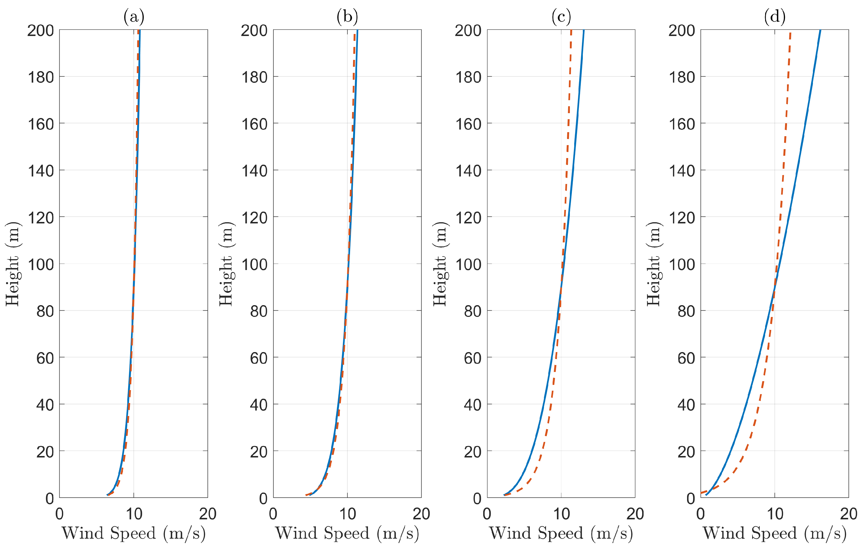
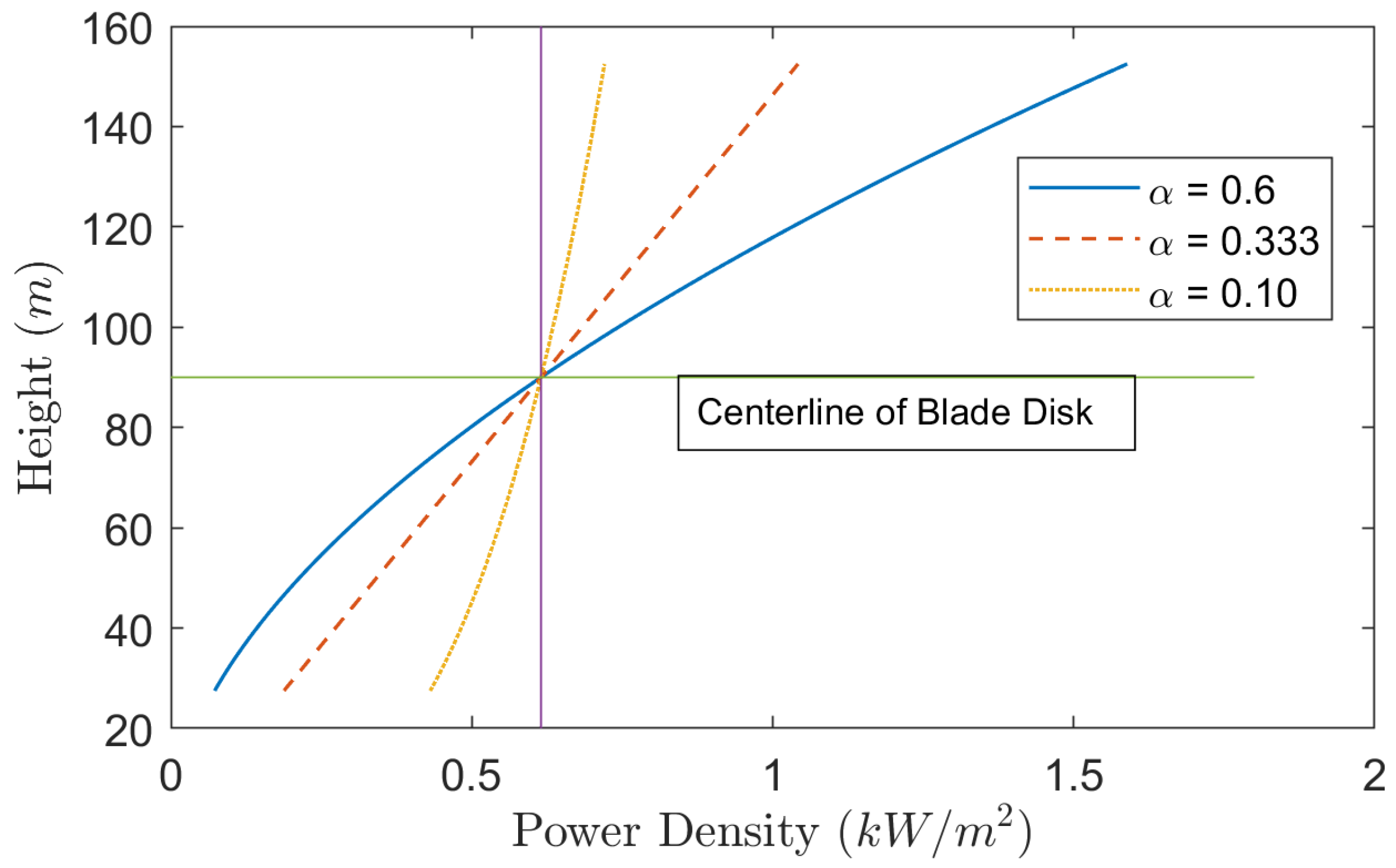
• Power Law Exponent Model: The power law exponent model [3,4,14] is an empirical equation which describes the wind speed in relation to a reference speed at a known altitude:

  $$V\left(h\right)=V_{10}{\left({\displaystyle \frac{h}{h_{10}}}\right)}^{\alpha },$$

  (1)

  where $V_{10}$ is the wind speed at a reference height $h_{10}$, which is usually taken to be 10 m, and $\alpha$ is the Hellmann exponent. The Hellmann exponent depends on the location, topology of the terrain, and atmospheric stability, referenced as turbulent air or neutral air. Table 1 [4,15] shows some examples of the Hellmann exponent.

  Table 1. Hellmann exponent examples.

  Location	$\mathit{\alpha }$
  Unstable air above open water	0.06
  Neutral air above open water	0.10
  Unstable air above flat, open coast	0.11
  Neutral air above flat, open coast	0.16
  Stable air above open water	0.27
  Unstable air above human-inhibited areas	0.27
  Neutral air above human-inhibited area	0.34
  Stable air above flat, open coast	0.40
  Stable air above human-inhibited areas	0.60

  Table 1. Hellmann exponent examples.

  Location	$\mathit{\alpha }$
  Unstable air above open water	0.06
  Neutral air above open water	0.10
  Unstable air above flat, open coast	0.11
  Neutral air above flat, open coast	0.16
  Stable air above open water	0.27
  Unstable air above human-inhibited areas	0.27
  Neutral air above human-inhibited area	0.34
  Stable air above flat, open coast	0.40
  Stable air above human-inhibited areas	0.60

• Logarithmic Model: A physical model of wind gradients is given by the logarithmic model [16,17,18]:

  $$V\left(h\right)=V\left(h_0\right)+{\displaystyle \frac{u^{*}}{\kappa }}\left[log\left({\displaystyle \frac{h}{z_0}}\right)-\psi \left({\displaystyle \frac{h}{L}}\right)\right],$$

  (2)

  where $V\left(h_0\right)$ is the wind speed at the reference altitude $h_0$, $z_0$ is the roughness length or roughness height, $\kappa$ is the Karman constant, and $u^{*}$ is the friction velocity. Atmospheric stability is included in this model using the function $\psi (·)$. In a neutral atmosphere, the above equation simplifies to

  $$V\left(h\right)=V\left(h_0\right){\displaystyle \frac{log\frac{h}{z_0}}{log\frac{h_0}{z_0}}}.$$

  (3)

  Typical values of $z_0$ have been estimated from experimental observations [5] to be in the range of 0.0001–2 m and above, where a higher value of $z_0$ indicates more obstructions to wind flow from, for example, trees and buildings. As in the case of the power law exponent model, the reference height $h_0$ is usually taken to be 10 m.

  Table 2. Example of roughness length values.

  Terrain	${\mathit{z}}_0$
  Open sea	0.0002
  Open mud flat, snow, no vegetation, no obstacles	0.005
  Open flat terrain, grass, few obstacles	0.03
  Low crop, some large obstacles	0.10
  High crop, scattered obstacles	0.25
  Parkland, bushes, many obstacles	0.5
  Large obstacles, forests	1.0
  City with high-rise buildings	>2.0

  [19] shows some typical values of the roughness length $z_0$.

Both wind gradient models provide a reasonable description of wind variation with height supported by observational data, but it is difficult to make a one-to-one comparison between the two models since the parameters $\alpha$ (Equation (1)) and $z_0$ (Equation (3)) have not been reported under the same physical conditions for the terrain. Nevertheless, the two models provide wind speed variations with the height which are similar or reasonably close, as shown in Figure 1.

The authors of [5,6] provided validity for the wind gradient models through observational data. LIDAR measurement data were used in [18] to validate the model in Equation (3). The authors of [20] presented a boundary layer model for wind turbine arrays typically found at wind farms and showed that optimal performance at wind farms occurs at a lower thrust coefficient than the Betz limit. Researchers have also considered these wind gradient models in various applications, such as the aerodynamic performance of conventional sails [21,22], gliding characteristics of fixed-wing UAVs [23,24], dynamic soaring of seabirds [25] and seaplanes [16], wind loading on structures [26], and windsail-assisted ship propulsion [27]. In recent years, individual blade pitch control has been proposed for wind load mitigation under wind shear [28,29].

The next section derives the new power coefficient for large horizontal axis wind turbines in the presence of wind gradient.

3. Power Coefficient for Large Wind Turbines

A simple model based on momentum theory and attributed to Betz [7] describes the maximum power which can be extracted from an ideal wind turbine [8], given by

$$P={\displaystyle \frac{1}{2}}{C}_p\rho A{V}^3,$$

(4)

where $\rho$ is the air density, A is the area of the cross-section of the swept area of the turbine blades (also known as the rotor disk or blade disk), and V is the wind speed. Based on the conservation laws of mass, linear momentum, and energy, the power coefficient has been shown to be $C_p={\displaystyle \frac{16}{27}}=0.593$, which is known as the Betz limit. While the Betz limit provides the aerodynamic maximum of the amount of power which can be extracted from wind, the actual extracted power can be much less because of the presence of a wake behind the blade disk and the design of the wind turbine.

The Betz limit is based on the assumption that the wind speed is uniform across the rotor disk, which may not hold for large wind turbines since wind gradient cause wind speeds to vary with the height. For example, a higher wind speed may be found at the top of a rotor disk compared with that near ground level. In what follows, we derive a new power coefficient for large horizontal-axis wind turbines based on variations in wind speed due to wind gradients.

Consider a wind turbine with a blade radius R at a given hub height $h_0$, shown in the Figure 2, and consider a thin slice of the rotor disk, as shown by the shaded area. Then, clearly we have

$$\begin{gathered} x=Rcos\theta , \\ y=Rsin\theta , \\ dy=Rcos\theta d\theta , \\ dA=2xdy=2R^2{cos}^2\theta d\theta . \end{gathered}$$

(5)

It is clear that the Betz limit holds for the infinitesimally thin slice $dA$ such that the maximum power which can be extracted is given by

$$dP={\displaystyle \frac{1}{2}}{C}_p\rho \left(dA\right)V^3\left(\theta \right),$$

(6)

where $C_p$ is the Betz constant and $V\left(\theta \right)$ is the wind speed as a function of the angle $\theta$. Clearly, $V\left(\theta \right)$ varies as the blade rotates in the disk. We assume that the air density $\rho$ is constant with the height within which wind turbines operate. Throughout this study, we assume an air density of 1.225 kg/m³ according to the International Standard Atmosphere at 101.325 kPa (abs) and 15 °C.

Using the power law exponent model in Equation (1) for the wind gradient, we express the wind velocity as

$$\begin{array}{cc}V\left(\theta \right)& =V_{10}{\left({\displaystyle \frac{h}{h_{10}}}\right)}^{\alpha }\hfill \\ & =V_{10}{\left({\displaystyle \frac{h_0+Rsin\theta }{h_{10}}}\right)}^{\alpha },-{\displaystyle \frac{\pi }{2}}\le \theta \le {\displaystyle \frac{\pi }{2}}\hfill \\ & =V_{10}{\left({\displaystyle \frac{h_0}{h_{10}}}\right)}^{\alpha }{\left(1+{\displaystyle \frac{R}{h_0}}sin\theta \right)}^{\alpha },\hfill \\ & =V_0{\left(1+{\displaystyle \frac{R}{h_0}}sin\theta \right)}^{\alpha },\hfill \end{array}$$

(7)

where $V_0$ is the wind speed at the rotor hub at a height $h_0$. Clearly, the above equation gives the variation in the wind speed with $\theta$ (i.e., along the height of the rotor disk).

When using the above equation in Equation (6), we have

$$\begin{array}{cc}dP& ={\displaystyle \frac{1}{2}}\rho C_p\left(dA\right)V_0^3{\left(1+{\displaystyle \frac{R}{h_0}}sin\theta \right)}^{3\alpha }\hfill \\ & ={\displaystyle \frac{1}{2}}\rho C_{p}2R^2{cos}^2\theta V_0^3{\left(1+{\displaystyle \frac{R}{h_0}}sin\theta \right)}^{3\alpha }d\theta ,\hfill \end{array}$$

(8)

and the total power which can be extracted from the rotor disk is given by

$$\begin{array}{cc}P& ={\displaystyle {\int }_{-{\displaystyle \frac{\pi }{2}}}^{{\displaystyle \frac{\pi }{2}}}}dP\hfill \\ & ={\displaystyle \frac{1}{2}}\rho C_p\pi R^2{V}_0^3{\displaystyle \frac{2}{\pi }}{\displaystyle {\int }_{-{\displaystyle \frac{\pi }{2}}}^{{\displaystyle \frac{\pi }{2}}}}{cos}^2\theta {\left(1+{\displaystyle \frac{R}{h_0}}sin\theta \right)}^{3\alpha }d\theta \hfill \\ & ={\displaystyle \frac{1}{2}}{\widehat{C}}_p\rho A{V}_0^3,\hfill \end{array}$$

(9)

where A is the area of the rotor disk and $V_0$ is the wind speed at the hub. In light of Equation (9), the power coefficient for a large wind turbine is given by

$${\widehat{C}}_p=C_p{\displaystyle \frac{2}{\pi }}{\int }_{-{\displaystyle \frac{\pi }{2}}}^{{\displaystyle \frac{\pi }{2}}}{cos}^2\theta {\left(1+{\displaystyle \frac{R}{h_0}}sin\theta \right)}^{3\alpha }d\theta .$$

(10)

For notational simplicity, we denote

$$\beta ={\displaystyle \frac{2}{\pi }}{\int }_{-{\displaystyle \frac{\pi }{2}}}^{{\displaystyle \frac{\pi }{2}}}{cos}^2\theta {\left(1+{\displaystyle \frac{R}{h_0}}sin\theta \right)}^{3\alpha }d\theta ,$$

(11)

and the modified power coefficient for large wind turbines can be expressed as follows:

$${\widehat{C}}_p=C_p\beta ,$$

(12)

where $C_p$ is the Betz constant. In case one ignores the wind gradient with the height, we have $\alpha =0$, therefore, $\beta =1$, which gives ${\widehat{C}}_p=C_P$, as expected.

While the modified power coefficient given by Equations (10) and (11) provides a closed-form solution for the maximum power which can be extracted using large wind turbines, we can find an approximate solution of the power coefficient which provides more insight into the power limit.

In Equation (11), we denote $x={\displaystyle \frac{R}{h_0}}sin\theta$, and then we have $\left|x\right|<1$ since ${\displaystyle \frac{R}{h_0}}<1$ for any horizontal-axis turbine structure. Thus, under the binomial theorem, we have

$${(1+x)}^n=1+nx+{\displaystyle \frac{n(n-1)}{2!}}{x}^2+{\displaystyle \frac{n(n-1)(n-2)}{3!}}{x}^3+\cdots$$

(13)

which is valid for non-integer exponents as well. In light of the above equation, we obtain

$${(1+{\displaystyle \frac{R}{h_0}}sin\theta )}^{3\alpha }=1+3\alpha {\displaystyle \frac{R}{h_0}}sin\theta +{\displaystyle \frac{3\alpha (3\alpha -1)}{2}}{\displaystyle \frac{R^2}{h_0^2}}{sin}^2\theta +\cdots$$

(14)

By using the above equation in Equation (11) and carrying out the integration, we obtain

$$\beta =1+{\displaystyle \frac{1}{2!}}·{\displaystyle \frac{1}{4}}·3\alpha (3\alpha -1)·{\displaystyle \frac{R^2}{h_0^2}}+{\displaystyle \frac{1}{4!}}·{\displaystyle \frac{1}{8}}·3\alpha (3\alpha -1)(3\alpha -2)(3\alpha -3)·{\displaystyle \frac{R^4}{h_0^4}}+\cdots ,$$

(15)

where we have shown the first three nonzero terms of the binomial expansion in Equation (14). All odd-degree terms of the expansion integrate to zero and are eliminated for clarity. Note that the above binomial series is convergent, and the value of $\beta$ depends on the Hellmann exponent $\alpha$. In particular, the value of $\alpha ={\displaystyle \frac{1}{3}}$ is a neutral exponent for which $\beta =1$. For $\alpha$ satisfying ${\displaystyle \frac{1}{3}}<\alpha <{\displaystyle \frac{2}{3}}$, all higher-order terms in the infinite series in Equation (15) (including those not shown) are positive and progressively smaller such that $\beta >1$. Likewise, for $\alpha$ satisfying $0<\alpha <{\displaystyle \frac{1}{3}}$, we have $\beta <1$, since all higher-order terms are negative and progressively smaller.

Table 3. Convergence of the infinite series in Equation (15) and the power coefficient.

	Terms in the Infinite Series (Equation (15))	Power Coefficient ${\widehat{\mathit{C}}}_{\mathit{p}}$
$\alpha =0.6$	Up to second-degree terms	0.64403
	Up to fourth-degree terms	0.64428
	Up to sixth-degree terms	0.64429
	Power coefficient based on Equation (10)	0.64430
	Betz limit	0.59259
$\alpha =0.1$	Up to second-degree terms	0.58509
	Up to fourth-degree terms	0.58440
	Up to sixth-degree terms	0.58434
	Power coefficient based on Equation (10)	0.58424
	Betz limit	0.59259

shows convergence of the infinite series in Equation (15), where we computed the true value of the power coefficient via numerical integration of Equation (10). It is also easy to see that the error in this approximation was about 0.042% for $\alpha =0.6$ and about 0.14% for $\alpha =0.10$. The known values of $\alpha$, as shown in Table 1, fell within the limit $0<\alpha <{\displaystyle \frac{2}{3}}$, and thus the above conclusions are broadly satisfied for all known terrains.

Next, we consider a truncated version of Equation (15) to provide additional insight into the power coefficient ${\widehat{C}}_p$. Since ${\displaystyle \frac{R}{h_0}}<1$, it is clear that the last term in Equation (15) is several orders of magnitude smaller than the second term. Furthermore, all successive higher-order terms (not explicitly shown in Equation (15)) are progressively smaller such that we can approximate

$$\beta \simeq 1+{\displaystyle \frac{3\alpha (3\alpha -1)}{8}}{\displaystyle \frac{R^2}{h_0^2}}.$$

(16)

This gives the modified power coefficient for large wind turbines, which is expressed as follows:

$${\widehat{C}}_p\simeq {\displaystyle \frac{16}{27}}\left(1+{\displaystyle \frac{3\alpha (3\alpha -1)}{8}}{\displaystyle \frac{R^2}{h_0^2}}\right).$$

(17)

While the above equation for the power coefficient is an approximate solution of the true solution in Equation (10) with a small error, it helps us understand how the power coefficient varies with various parameters, such as the blade length, hub height, and the Hellmann exponent. Figure 3 shows the variation in the power coefficient with the terrain which is described by the Hellmann exponent. As discussed earlier, neutral air in open ocean or flat land signifies smaller value of $\alpha$, and the corresponding value of the power coefficient ${\widehat{C}}_p$ is smaller than that predicted by the Betz limit. Also, recall that for neutral air in human inhibited-areas, $\alpha ={\displaystyle \frac{1}{3}}$, and the power coefficient ${\widehat{C}}_p$ is same as the Betz limit. For stable air in open coast and human-inhibited areas, $\alpha >{\displaystyle \frac{1}{3}}$, and thus ${\widehat{C}}_p>C_p$.

In Figure 4, we show the power coefficient ${\widehat{C}}_p$ as a function of the ratio ${\displaystyle \frac{R}{h_0}}<1$ for different values of the Hellman exponent $\alpha$, where we assumed that the height of the turbine hub $h_0$ was fixed. As shown in the figure, for $\alpha =0.6$, a longer blade length (i.e., larger ${\displaystyle \frac{R}{h_0}}$) signifies a larger power coefficient ${\widehat{C}}_p$ compared with the Betz limit. For a smaller rotor disk (i.e., smaller ${\displaystyle \frac{R}{h_0}}$), the wind speed is relatively uniform across the disk such that ${\widehat{C}}_p$ is almost the same as the Betz limit. On the other hand, for offshore turbines with $\alpha =0.10$, the power coefficient ${\widehat{C}}_p$ is slightly smaller than the Betz limit. For $\alpha ={\displaystyle \frac{1}{3}}$, the power coefficient ${\widehat{C}}_p$ is the same as the Betz limit, which follows from Equation (17).

It is also interesting to see the effect of the wind gradient on the power density across a rotor disk. In Figure 5, we plot the power density ($P={\displaystyle \frac{1}{2}}\rho V^3$) of the rotor disk versus the height, using the reference wind speed $V_0$ = 10 m/s at a hub height of $h_0$ = 90 m and a rotor radius of R = 62.5 m.

Because of the wind gradient, the wind speed in the upper half of the rotor disk is higher than that in the lower half. This leads to a corresponding variation in the power density across the rotor disk, as shown in Figure 5. In general, the power density in the upper half of the rotor disk is greater than that at the hub, and the power density in the lower half is less than that at the hub. Furthermore, such variations in the power density depend on the Hellmann exponent $\alpha$. For $\alpha ={\displaystyle \frac{1}{3}}$, a higher power density above the hub is balanced out by a loss of power density below the hub, as shown by the dotted line in Figure 5, such that ${\widehat{C}}_p=C_p$. On the other hand, for $\alpha =0.6$, a higher power density in the upper half of the rotor disk outweighs the loss of the power density below the hub, which justifies why ${\widehat{C}}_p$ is greater than the Betz coefficient. Likewise, for $\alpha =0.10$, there is a greater loss of power density in the lower half of the rotor disk compared with the upper half, which signifies a lower value of ${\widehat{C}}_p$. This shows that offshore wind turbines are likely to generate less power compared with their onshore counterparts for the same size.

Table 4. Wind power for $V_0$ = 10 m/s, $h_0$ = 90 m, and R = 62.5 m.

	Average Power Density (kW/m2)			Total Power (MW)
Hellmann Exponent	Upper Half of Rotor Disk	Lower Half of Rotor Disk	Hub	Total Power Available in Rotor Disk	Maximum Extractible (This Paper)	Maximum Extractible (Betz Limit)
0.6	0.993	0.344	0.615	8.2057	5.2845	4.4679
$0.333$	0.796	0.433	0.615	7.5472	4.4679	4.4679
$0.10$	0.663	0.549	0.615	7.4408	4.3536	4.4679

shows the average power densities and total power extractible for various values of $\alpha$.

Although offshore turbines have a lower average power density compared with onshore turbines, the availability of higher wind speeds may offset this disadvantage. As depicted in Figure 6, the average offshore wind speed at 90 m rose from less than 8 m/s near the shore to greater than 10 m/s at 100 km offshore [30]. Assuming that the mean wind speed is linearly dependent on the distance from the shore, along with the modified power coefficient ${\widehat{C}}_p$ from Equation (17), the wind power as a function of the distance from the shore can be determined. As shown in Figure 7, the power generated by the offshore wind turbine (used in this study) increased from 2.25 MW above flat, open coast to 4.43 MW above open ocean 100 km from the shore. Additionally, offshore winds are more consistent, resulting in a higher capacity factor, as shown by recent advancements in offshore wind farms worldwide [31].

4. Discussions

In light of the above analysis, a few comments are in order. First of all, a closed-form solution of the modified power coefficient for large wind turbines is given by Equation (10). A more useful and better approximation of the modified power coefficient can be given by ${\widehat{C}}_p=C_p\beta$, where $\beta$ is given by Equation (16) and $C_p$ is the Betz constant. In a case where one ignores the wind gradient, we have ${\widehat{C}}_p=C_p$, which is also satisfied if $\alpha ={\displaystyle \frac{1}{3}}$. The value of $\beta$ depends on the wind gradient profile based on the location and stability of the wind.

If the Hellmann exponent is within the range of ${\displaystyle \frac{1}{3}}<\alpha <{\displaystyle \frac{2}{3}}$, we have ${\widehat{C}}_p>C_p$ (i.e., the power extracted using large wind turbines could be more than that predicted by the Betz limit). For example, the Hellmann exponent for stable air above flat, open coast line was $\alpha =0.40$. Assuming a disk diameter of $2R$ = 125 m and a rotor hub height $h_0$ = 90 m, we obtain $\beta =1.0149$, which gives a modified power limit of ${\widehat{C}}_p=0.601$. For stable inland air, $\alpha =0.6$, which gives $\beta =1.0873$ and ${\widehat{C}}_p=0.644$, which is about 8.73% above the Betz limit.

On the other hand, for $\alpha <{\displaystyle \frac{1}{3}}$, we have ${\widehat{C}}_p<C_p$, signifying less power extraction compared with the Betz limit. Consider, for example, a wind turbine in stable air above an open water surface with the Hellmann exponent $\alpha =0.27$, which gives $\beta =0.9902$ and ${\widehat{C}}_p=0.5868$, which is about 1% less than that predicted by the Betz limit. For neutral air in open ocean, $\alpha =0.10$, which gives $\beta =0.9873$ and a corresponding value of ${\widehat{C}}_p=0.5851$ for the power coefficient, which is about 1.27% less than the Betz limit. In other words, the maximum power extracted by offshore large wind turbines is smaller than that predicted by the Betz coefficient. The loss of 1.27% for the power coefficient may, however, be offset by more consistent and higher average wind speeds for offshore wind turbines.

While the Betz limit is valid for both horizontal-axis and vertical-axis wind turbines, the analytical approach used in this paper applies to horizontal-axis wind turbines only. In particular, the derivation of the power coefficient presented in Section 3 assumes that the rotor disk is of a certain radius R located at a hub height of $h_0$, as shown Figure 2, which does not hold for vertical-axis wind turbines. Nevertheless, the wind gradient in relation to the height applies, which justifies higher wind speeds in the upper half of the rotor plane compared with those in the lower half. Thus, the power coefficient of vertical-axis wind turbines is likely to be different from that predicted by the Betz limit. This will be the subject of future research.

Figure 8 shows the power coefficients of some common wind turbines as a function of the blade tip speed ratio [32]. Modern three-blade wind turbines are known to be the most efficient ones, with a power coefficient of about 40–50%, which is less than the Betz limit. For other types of turbines, the actual power coefficient is even less. Our results are also derived based on the same basic aerodynamic assumptions as the Betz limit, and thus the actual power coefficient of horizontal-axis wind turbines in the presence of a wind gradient is expected to remain in the same ballpark from approximately $-1.27\%$ to $8.73\%$ of those shown in Figure 8. Although the air density may vary slightly at offshore and onshore installations due to moisture contents, its effect on the power coefficient is not significant.

5. Conclusions

It is known that the wind speed is not constant at all heights from the Earth’s surface; rather, it shows a gradient profile based on surface friction and daily thermal heating and cooling due to sunlight. Considering the power exponent model of wind gradients, we derived a new power coefficient for large horizontal-axis wind turbines which varies with the location and stability of the air, as opposed to the fixed power coefficient given by the Betz limit. Contrary to the Betz limit, the power coefficient derived in this paper gives an estimate of how much power can be extracted from wind when the wind speed varies across a blade disk. Common factors which reduce the power coefficient include rotating wake formation behind the blade disk, the blade design, turbulence due to the support structure, and the ratio of the blade tip speed to the wind speed. Our results show that the power coefficient for large wind turbines at onshore locations exceeded the Betz limit by about 8.7%, while the power coefficient for offshore turbines could be about 1.27% smaller. In short, the developed power coefficient for wind turbines is a generalization of the well-known result of the Betz limit through elimination of the assumption of a constant wind speed across the blade disk, and secondly, wind power companies may find our results helpful in selecting the best locations for installing new wind turbines, potentially achieving higher power output than that predicted by the Betz limit.

References

1. International Renewable Energy Agency. Available online: https://www.irena.org/Energy-Transition/Technology/Wind-energy (accessed on 6 July 2024).
2. US Department of Energy. Available online: https://www.energy.gov/eere/articles/wind-turbines-bigger-better (accessed on 17 June 2024).
3. Harrison, R.; Hau, E.; Snel, H. Large Wind Turbines: Design and Economics; John Wiley: Hoboken, NJ, USA, 2001. [Google Scholar]
4. Kaltschmitt, M.; Streicher, W.; Wiese, A. Renewable Energy Technology, Economics and Environment; Springer: Berlin/Heidelberg, Germany, 2007. [Google Scholar]
5. Stull, R.B. An Introduction to Boundary Layer Meteorology; Kluwer Academic Publishers: London, UK, 1997. [Google Scholar]
6. Li, Q.; Zhi, L.; Hu, F. Boundary Layer Wind Structure from Observations on a 325m Tower. J. Wind. Eng. Ind. Aerodyn. 2010, 98, 818–832. [Google Scholar] [CrossRef]
7. Betz, A. Das Maximum der theoretischen Ausnutzung des Windes durch Windmotoren. Z. Für Das Gesamte Turbinenwesen 1920, 26, 307–309. [Google Scholar]
8. Manwell, J.F.; Branlard, E.; McGowan, J.G.; Ram, B. Wind Energy Explained: On Land and Offshore, 3rd ed.; Wiley: Hoboken, NJ, USA, 2024. [Google Scholar]
9. Vennel, R. Exceeding the Betz limit with tidal turbines. Renew. Energy 2013, 55, 277–285. [Google Scholar] [CrossRef]
10. Liew, J.; Heck, K.S.; Howland, M.F. Unified momentum model for rotor aerodynamics across operating regimes. Nat. Commun. 2024, 15, 6658. [Google Scholar] [CrossRef] [PubMed]
11. Madsen, H.A.; Larsen, T.J.; Pirrung, G.R.; Li, A.; Zahle, F. Implementation of the blade element momentum model on a polar grid and its aeroelastic load impact. Wind Energ. Sci. 2020, 5, 1–27. [Google Scholar] [CrossRef]
12. Moriarty, P.J.; Hansen, A.C. Aerodyn Theory Manual. 2005. Available online: https://www.nrel.gov/docs/fy05osti/36881.pdf (accessed on 8 December 2024).
13. Chen, J.S.; Chen, Z.; Biswas, S.; Miau, J.; Hsieh, C. Torque and Power Coefficients of a Vertical Axis Wind Turbine With Optimal Pitch Control. In Proceedings of the ASME 2010 Power Conference, Chicago, IL, USA, 13–15 July 2010; pp. 655–662. [Google Scholar] [CrossRef]
14. Heier, S. Grid Integration of Wind Energy Conversion Systems; Wiley: Hoboken, NJ, USA, 2005; ISBN 978-0-470-86899-7. [Google Scholar]
15. Hsu, S.A. Coastal Meteorology; Academic Press: London, UK, 1988. [Google Scholar]
16. Sukumar, P.; Selig, M.S. Dynamic Soaring of Sailplanes over Open Fields. J. Aircr. 2013, 50, 1420–1430. [Google Scholar] [CrossRef]
17. van den Berg, G.P. Wind gradient statistics up to 200 m altitude over flat ground. In Proceedings of the First International Meeting on Wind Turbine Noise: Perspectives for Control, Berlin, Germany, 17–18 October 2005. [Google Scholar]
18. Houshuo, J.H.; James, B.; Edson, J.B. Characterizing marine atmospheric boundary layer to support offshore wind energy research. J. Physics Conf. Ser. 2020, 1452, 012027. [Google Scholar]
19. Wieringa, J. Updating the Davenport Roughness Classification. J. Wind. Eng. Ind. Aerodyn. 1992, 41, 357–368. [Google Scholar] [CrossRef]
20. Li, C.; Liu, L.; Lu, X.; Stevens, R.J.A.M. Analytical model of fully developed wind farms in conventionally neutral atmospheric boundary layers. J. Fluid Mech. 2022, 948, A43. [Google Scholar] [CrossRef]
21. Wen-Ring, H.; Hong-Biao, Z.; Zu-Rong, D. Computational Study of the Aerodynamics of Sails in a Twisted Wind. J. Shanhgai Jiaotong Univ. 2008, 42, 1900–1903. [Google Scholar]
22. Mortimer, I.A. A Comparison of Downwind Sail Coefficients from Tests in Diffeent Wind Tunnels. Ocean. Eng. 2014, 90, 62–71. [Google Scholar] [CrossRef]
23. Bower, G.C. Boundary Layer Dynamic Soaring for Autonomous Aircraft Design and Validation. Ph.D. Thesis, Stanford University, Stanford, CA, USA, 2011. [Google Scholar]
24. Deittert, M.; Richards, A.; Toomer, C.A.; Pipe, A. Engineless Unmanned Aerial Vehicle Propulsion dy Dynamic Soaring. J. Guid. Control. Dyn. 2009, 32, 1446–1457. [Google Scholar] [CrossRef]
25. Sachs, G.; Bussotti, P. Application of Optimal Control Theory to Dynamic Soaring of Seabirds. In Variational Analysis and Applications; Giannessi, F., Maugeri, A., Eds.; Springer: New York, NY, USA, 2005; Volume 79, pp. 975–994. [Google Scholar]
26. Holmes, D. Wind Loading of Structures; Spon Press: New York, NY, USA, 2001. [Google Scholar]
27. Li, C.; Wang, H.; Sun, P. Study on the Influence of Gradient Wind on the Aerodynamic Characteristics of a Two-Element Wingsail for Ship-Assisted Propulsion. J. Mar. Sci. Eng. 2023, 11, 134. [Google Scholar] [CrossRef]
28. Suemoto, H.; Hara, N.; Nihei, Y.; Konishi, K. Experimental Testing on Blade Load Mitigation of wind Turbines with Individual Blade Pitch Control under Wind Shear. In Proceedings of the IEEE 4th International Conference on Advanced Robotics and Mechatronics, Toyonaka, Japan, 3–5 July 2019. [Google Scholar] [CrossRef]
29. Kotur, D.; Durišić, Z. Individual Pitch Control for Wind Turbine Load Reduction Recognizing Atmospheric Stability. In Proceedings of the Wind Europe Summit 2016, Hamburg, Germany, 27–30 September 2016. [Google Scholar]
30. Offshore Wind. Available online: https://atb-archive.nrel.gov/electricity/2019/index.html?t=ow&s=ov (accessed on 14 January 2025).
31. Jung, C.; Schindler, D. The Properties of the Global Wind Turbine Fleet. Renew. Sustain. Energy Rev. 2023, 186, 113667. [Google Scholar] [CrossRef]
32. Ebrahimpour, M.; Shafaghat, R.; Alamian, R.; Safdari, M.S. Numerical Investigation of the Savonius Vertical Axis Wind Turbine and Evaluation of the Effect of the Overlap Parameter in Both Horizontal and Vertical Directions on Its Performance. Symmetry 2019, 11, 821. [Google Scholar] [CrossRef]
Figure 1. Comparison of wind gradient models. Solid line = power law exponent model; dotted line = logarithmic model. (a) Open oceans ( α = 0.1 , z 0 = 0.0002 ) . (b) Neutral air for flat, open coast ( α = 0.16 , z 0 = 0.03 ) . (c) Neutral air in human-inhibited area ( α = 0.333 , z 0 = 0.25 ) . (d) Stable air in human-inhibited area ( α = 0.6 , z 0 = 2.0 ) .
Energies 18 00740 g001
Figure 2. Schematic of a large wind turbine.
Energies 18 00740 g002
Figure 3. Power coefficient with Hellmann exponent α .
Energies 18 00740 g003
Figure 4. Power coefficient as a function of the ratio R h 0 .
Energies 18 00740 g004
Figure 5. Variation in power density with height for V 0 = 10 m/s, h 0 = 90 m, and R = 62.5 m.
Energies 18 00740 g005
Figure 6. Average wind speed at US shoreline at a height of 90 m [30].
Energies 18 00740 g006
Figure 7. The maximum wind power (MW) as a function of the distance from the shore, with V 0 = 8 m/s at the shore, V 0 = 10 m/s at 100 km offshore, h 0 = 90 m, and R = 62.5 m.
Energies 18 00740 g007
Figure 8. Power coefficients of various wind turbines in comparison with the Betz limit [32]. Dashed line shows the Betz limit.
Energies 18 00740 g008