Investigations on the Aerodynamic Interactions Between Turbine and Diffuser System by Employing the Kriging Method

Abstract

An exhaust diffuser determines the turbine outlet pressure by recovering kinetic energy. Conversely, the distributions of the total pressure and flow directions at the turbine exit affect the aerodynamic performance of the exhaust diffuser. As the output power increases gradually, the structure of the modern gas turbine becomes more compact. Consequently, the coupled effect of the flow in the last-stage turbine and the exhaust diffuser becomes increasingly obvious. Understanding the correlation between the flow field and the performance of the coupled system is of great significance. As a predictive regression algorithm, the Kriging method is widely used due to its high efficiency and unique mathematical characteristics. In this paper, computational fluid dynamics (CFD) numerical simulation is employed to investigate the interactions between the flow fields of the coupled system, and the corresponding datasets are obtained. Accordingly, the Kriging method is successfully employed to reconstruct the complex flow field, and a quantitative model describing the interaction between the two parts is established. This paper provides a detailed summary of the interaction between the flow field in the exhaust diffuser and the flow field at the outlet of the last-stage turbine. Through the prediction of the flow field, the conditions that induce the separation vortex on the casing of the diffuser are determined. Specifically, the slope of the total pressure change along the blade height near the casing is found to be k = −4.37.

1. Introduction

In a gas turbine, the diffuser system determines the turbine outlet pressure by recovering kinetic energy. Numerous studies and measured data from actual operating conditions show that there is a strong interaction between the flow field of the last-stage turbine and the diffuser system. This interaction affects not only the aerodynamic performance of the turbine and diffuser system but also the safety of the blades.

The inflow characteristics at the turbine exit, including tip leakage, total pressure, swirl angle, and turbulence intensity, have a great influence on the flow structures in diffusers. In the actual operation of gas turbines, the upstream blade wake flow field can still be detected in the exhaust diffuser [1]. Babu [2,3] found that for tip leakage, there is an optimal value for the inhibition of separation exhibited by struts. Zimmermann [4] confirmed that the performance improvement of the diffuser is insufficient to compensate for the increased losses in the turbine due to the large tip clearance. Vassiliev [5] concluded that the non-uniform inlet pressure distribution enables the diffuser to achieve better performance. David and Alexander [6] found that the non-uniform circumferential inlet conditions have a great influence on the diffuser performance. Drechsel [7,8] and Stevens [9] pointed out that greater turbulent kinetic energy near the casing at the turbine outlet results in a higher static pressure recovery coefficient. Vassiliev [10] confirmed that the turbulent flow at the turbine outlet is beneficial for suppressing flow separation and reducing the area of the flow separation zone, thereby enhancing pressure recovery and shortening the length of the diffuser. Vassiliev et al. [11] found that the swirl at the turbine outlet is generally beneficial for improving the diffuser performance.

Due to the high complexity of the flow field in turbine and diffuser system, it is often necessary to use computational fluid dynamics (CFD) software to solve the Navier–Stokes (N-S) equations. When steady or unsteady 3D simulations are employed, each evaluation of the N-S equations may entail a significant computational cost. Motivated by the need for research progress, a computationally efficient framework for reliability analysis was developed. Several authors have proposed various data processing methods to quickly predict the performance and aerodynamic parameters of gas turbines. Elias Tsoutsanis [12] predicted engine behavior using the Derivative-Driven Window-Based Regression method and demonstrated the improved accuracy of their methodology. Huang [13] developed a design optimization method to provide rapid approximations of time-consuming computations using the Kriging surrogate model. Wang [14] established a global mapping between design variables and objective functions using the Kriging model, which serves as a surrogate model. It is evident that the Kriging model not only possesses high flexibility but also effectively balances computational accuracy and efficiency. This is why it is extensively employed as a surrogate for implicit function models.

In this study, a Kriging surrogate model was constructed using Python SmartUQ (Version 7.0, manufacture by Shanghai Feiyi Software Technology Co., Ltd., Shanghai, China) to describe the interactions between the flow fields in the turbine and diffuser system and to predict their performance. The coupled aerodynamic performance was investigated to find out the key flow characteristics that determine the flow structure and performance in the turbine and diffuser. The key flow characteristics of the last-stage turbine were taken as input, while the flow field distributions in the diffuser were taken as outputs. The Kriging kernel function was set as Matérn functions to train the surrogate model. Then, the leave-one-out method is used to cross-validate the model and confirm the accuracy. Finally, the Kriging surrogate model with high prediction accuracy was obtained.

2. Simulation and Test

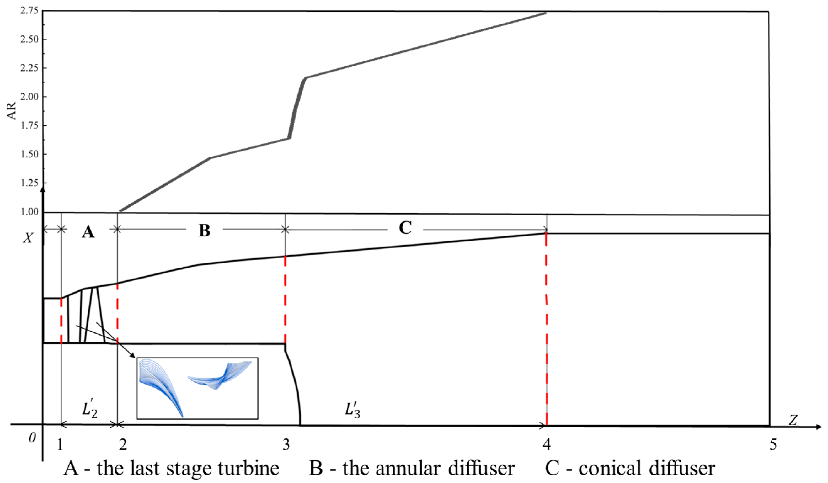
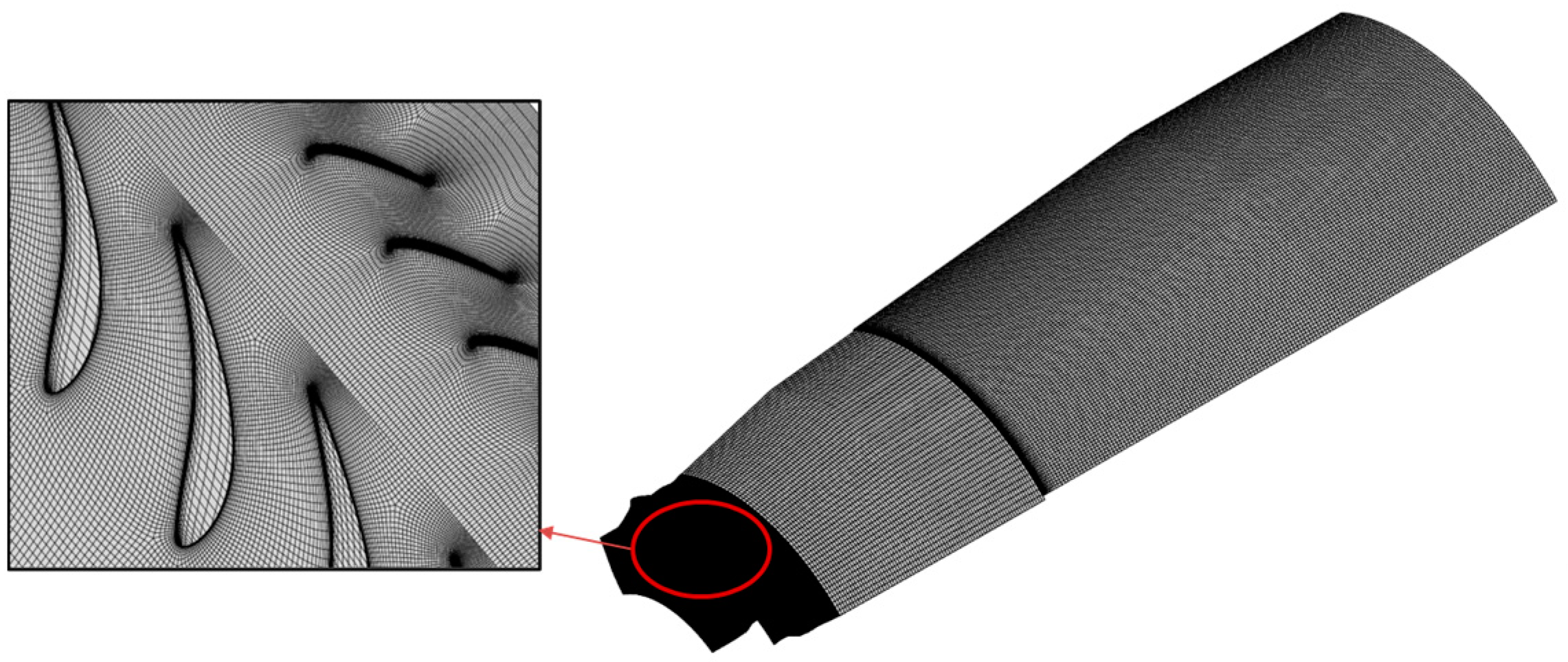
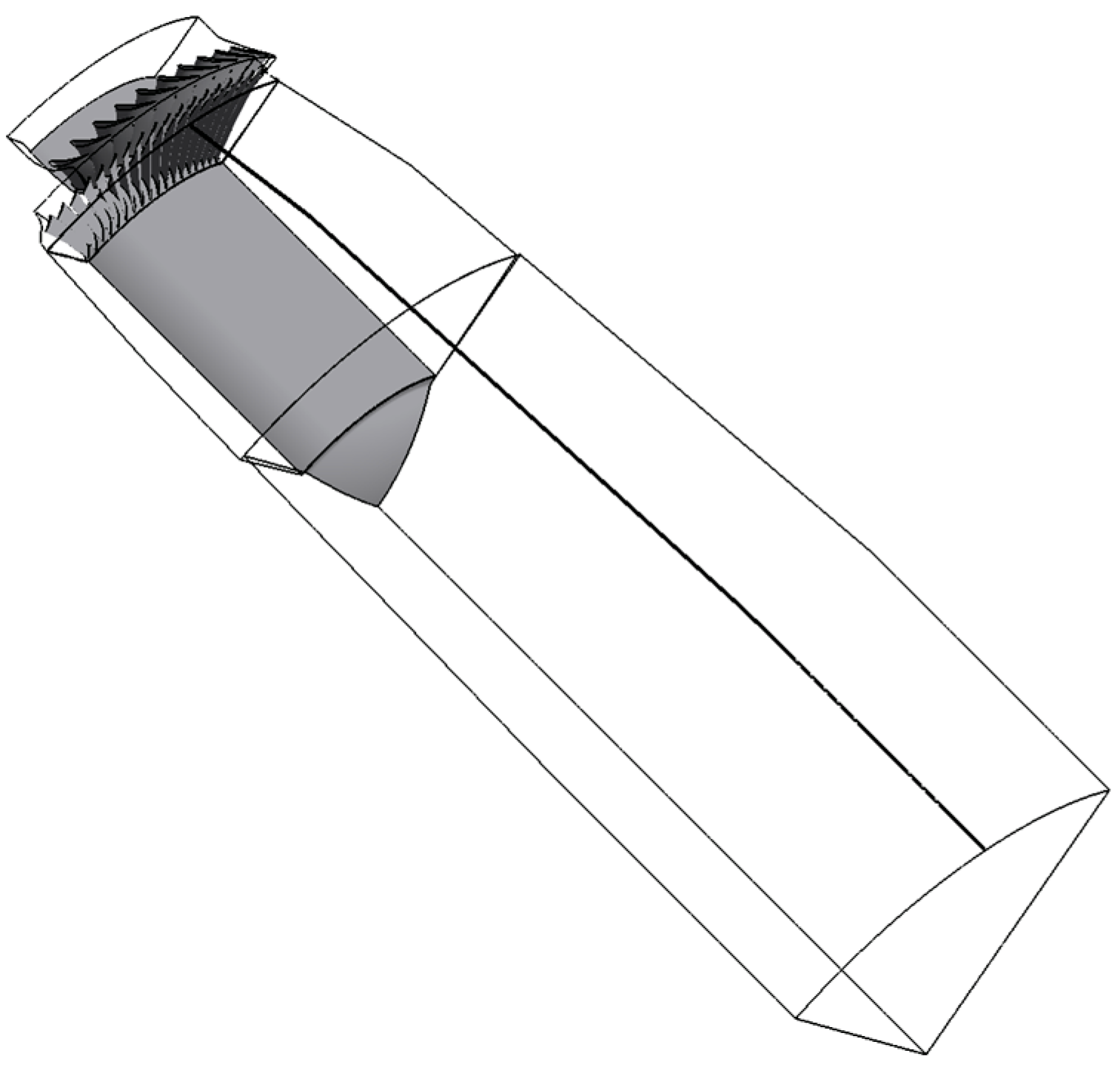
2.1. Geometric Models and Numerical Simulation Methods

A typical full-scale diffuser model of a heavy-duty gas turbine was chosen to numerically study the flow interactions between the last-stage turbine and the diffuser. The hubs of the last-stage turbine and the annular diffuser are both cylindrical, with a diameter of 2143 mm. The casing is expanded, and the turbine outlet diameter is 3686 mm. The heights of the stator and rotor blade are 658 mm and 732 mm, respectively, and the chord lengths are 180 mm and 263 mm, respectively. The angle between the diffuser casing and the central axis is 13°, and the total length of the exhaust diffuser is 5600 mm.

Given that the ratio of the stator to rotor blades is about 5:9 for real units, the numbers of stator and rotor blade passages were set as 10 and 18, respectively, for the CFD simulation. The tip clearance of the rotor is 1.9% of the height of the rotor blade. The calculation domain, as shown in Figure 1, consisted of the last-stage turbine passages, the annular diffuser, and the conical diffuser. This study focuses on the last-stage turbine and the exhaust diffuser without a strut. The area ratio (AR) represents the ratio of a specific cross-sectional area to the inlet area of the diffuser. Axial section positions 0 to 5 represent the computational domain inlet, the last-stage turbine inlet, the exhaust diffuser inlet, the annular diffuser outlet, the conical diffuser outlet, and the computational domain outlet, respectively. The relative axial positions $L_2^{\prime }$ and $L_3^{\prime }$ in the diffuser are defined by Equations (1) and (2). The static pressure coefficient ($C_P$), total pressure coefficient ($C_{tp}$), static pressure recovery coefficient ($C_{pr}$), and total pressure loss coefficient ($C_{tpl}$) used in this paper are defined in Equations (3)–(6).

$$L_2^{\prime }=(Z-Z_1)/(Z_2-Z_1)$$

(1)

$$L_3^{\prime }=(Z-Z_2)/(Z_3-Z_2)$$

(2)

$$C_P=(P-\overline{P_2})/(\overline{P_{t2}}-\overline{P_2})$$

(3)

$$C_{tp}=\left(P_t-\overline{P_{t2}}\right)/\left(\overline{P_{t2}}-\overline{P_2}\right)$$

(4)

$$C_{pr}=(\overline{P}-{\bar{P}}_2)/({\bar{P}}_{t2}-{\bar{P}}_2)$$

(5)

$$C_{tpl}=({\bar{P}}_{t2}-{\bar{P}}_t)/({\bar{P}}_{t2}-{\bar{P}}_2)$$

(6)

where Z is the axial position; $P_t$ is the total pressure; $P$ is the static pressure; and the subscripts 1, 2, and 3 are shown in Figure 1.

The 3D steady-state simulations of the coupled flow field in the turbine and diffuser system were conducted by using the commercial computational fluid dynamics software CFX 2021 (Version 2021, manufactured by ANSYS, Inc., Canonsburg, PA, USA). The spatial discretization was second-order accurate. The fluid was considered an ideal gas. The airflow direction was set perpendicular to the domain inlet and the turbulence intensity was set to 5% for inlets without specified turbulence requirements. The rotor blade speed was maintained at 3000 rpm across different conditions. Because the circumferential difference in the flow field at the turbine outlet needs to be considered in the research, the interface of the rotor and stator was selected as the frozen rotor interface. The end-wall was set as smooth and non-slip. The distributions of the total pressure and total temperature were specified as uniform at the inlet. Three different operational conditions were established, as shown in

Table 1. Inlet total pressure for different operational conditions.

Case	${\mathit{P}}_{01}/{\mathit{P}}_{\mathit{a}\mathit{t}\mathit{m}}$	Case	${\mathit{P}}_{01}/{\mathit{P}}_{\mathit{a}\mathit{t}\mathit{m}}$	Case	${\mathit{P}}_{01}/{\mathit{P}}_{\mathit{a}\mathit{t}\mathit{m}}$
1	1.579	2	1.974	3	2.270

, to analyze the qualitative evolution of the internal flow characteristics of the turbine and diffuser with changes in inlet pressure. The total inlet pressure ($P_{01}$) of the three operational conditions is different, while the inlet temperature ($T_{01}$) remains the same. The outlet is set to the same pressure conditions, and the outlet static pressure ($P_{atm}$) is maintained as atmospheric pressure.

Structured meshes of the conical diffuser were generated separately using ICEM CFD (Version 2021, manufactured by ANSYS, Inc., Canonsburg, PA, USA). NUMECA-AutoGrid (Version 102, manufactured by NUMECA International, Brussels, Belgium) was chosen to generate the structured meshes for the last-stage turbine and the annular diffuser because it can produce high-quality structured meshes quickly using a variety of prebuilt turbomachinery grid templates. To achieve a good boundary layer flow simulation, finer meshes were employed near the end-wall. Figure 2 shows the grid arrangement for the entire domain.

Table 2. The geometry of the last-stage turbine and the exhaust diffuser.

	Stator	Rotor	Diffuser
Number of passages	10	18	1
The circumferential angle of the domain	72°	72°	72°

shows the geometric information and meshes for each part of the computational domain.

The mesh numbers for the computational domains were determined through a grid independency test. The results are shown in Figure 3. The static pressure recovery coefficients of the diffuser were compared across different mesh sizes. It was found that the static pressure recovery coefficient increases with the number of grid nodes and tends to be constant. Therefore, 14.4 million grids were selected for the subsequent numerical calculations in this paper. The final grid counts are shown in

Table 3. The meshes of the last-stage turbine and the exhaust diffuser.

	Stator	Rotor	Diffuser
Number of nodes	2.62 million	8.15 million	3.63 million

.

2.2. Test Method

To validate the numerical method, the test was conducted in the test section shown in Figure 4. The test section comprises a 1/14-scale model of an axial flow exhaust diffuser, along with an inlet grid and vanes, A-A represents the right view at A. Total pressure probes, thermocouples, and static pressure holes were used to measure the total pressure, total temperature, and static pressure upstream. A five-hole probe was used to record the radial distribution of total pressure and flow angle at the inlet and outlet of the diffuser. Static pressure at the casing of the conical diffuser and at different spans of struts in the annular diffuser was obtained by using wall static pressure holes. The pressures measured by the probe and sensed through the wall static pressure holes are collected by Honeywell sensors, with a measurement error of ±1 Pa. The positional error of the five-hole probe is ±0.05 mm. The parameters obtained by the probe were averaged using Equation (7).

$$a={\displaystyle \frac{\sum (a\times {\dot{m}}_l)}{\sum \left({\dot{m}}_l\right)}}$$

(7)

where $a$ represents a parameter in the flow field, $\dot{m}$ is the mass flow rate, and the subscript l represents the local value.

The static pressure holes on the casing of the conical diffuser are distributed circumferentially over a 72° sector between the two struts, arranged in sets every 18° along the circumference, with a total of three sets. Each group has eight holes uniformly arranged in the flow direction. The static pressure holes on the strut of the annular diffuser are arranged along the surface of the strut. At positions of the span = 0.1, 0.5, and 0.9, 7 holes are arranged on each side of the strut.

The operational conditions involved in the test are consistent with those listed in Table 1. The computed local static pressure recovery coefficient, referenced to the diffuser inlet, has been compared with the experimental data, as shown in Figure 5. Clearly, although the results of the simulation and the experiment have somewhat different characteristics, the numerical results and the experimental data agree well in terms of the overall trend. The discrepancies resulting from the k-e turbulence model are the slightest. The maximum error for point measurements is 3.2%, and the maximum relative error of the average value on the planes is 5.9%. This is because the vortices in the conical diffuser are much stronger, which makes it difficult to simulate and measure accurately. Nevertheless, the comparisons shown in Figure 6 demonstrate the reliability of the numerical simulation results. The standard k-ε turbulence model is used for the simulations in this paper.

3. The Flow Field in Diffuser Changes with the Operational Conditions

3.1. Flow Field in the Last-Stage Turbine

Figure 6 compares the total pressure coefficient and streamlines at the turbine outlet under different operational conditions. As $P_{01}/P_{atm}$ increases, the non-uniformity of the total pressure at the turbine outlet increases. The region of the total pressure peak value gradually changes from the center of the span to the hub. The total pressure at the casing decreases continuously, and the circumferential fluctuation of pressure at the hub is more pronounced. With the increase of $P_{01}/P_{atm}$, the direction of airflow at the turbine outlet gradually changes from tangential to radial. In Case 3, the secondary flow in the rotor passage continuously affects the turbine outlet, and the airflow direction changes from circumferential to radial.

Figure 7 shows the radial distributions of axial Mach number (${Ma}_z$), absolute tangential flow angle ($\theta$), and total pressure coefficient at the turbine outlet under three operational conditions. Clearly, the axial velocity gradually decreases from the hub to the tip of the blade passage. With the increase of $P_{01}/P_{atm}$, the axial velocity values near the casing remain nearly constant due to the blockage in the rotor passages. However, the axial Mach number at the hub increases by 50%, which results in a more negative gradient of axial velocity along the radial direction. From Case 1 to Case 3, the tangential flow angle gradually decreases. In Case 3, the tangential flow angle at the outlet is close to 0°, as shown in Figure 7. The negative gradient of the total pressure at the turbine outlet in the radial direction increases as the inlet total pressure increases.

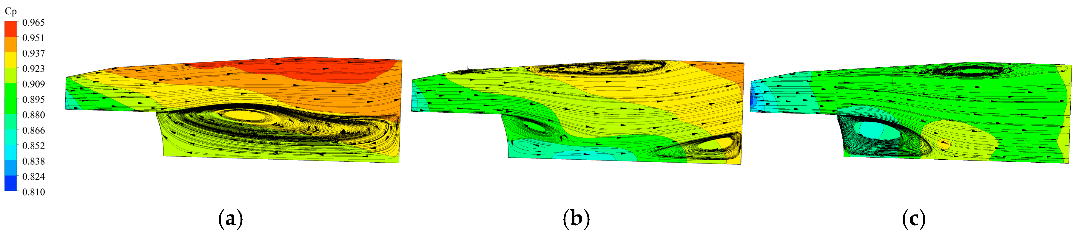
3.2. Flow Field in the Exhaust Diffuser

Figure 8 shows the static pressure recovery and the total pressure loss coefficient of the exhaust diffuser along the axis under the three operational conditions. Under different operational conditions, the difference between the actual pressure recovery coefficient and the ideal pressure recovery coefficient ($C_{prideal}$) of the annular diffuser is mainly observed in the range of $L_3^{\prime }$ = 3/4–4/4. The pressure recovery coefficient in this part of the annular diffuser increases gradually with the increase in the pressure ratio. The diffuser maintains its diffusing efficiency throughout the conical diffuser in Case 1. In Case 2, the pressure recovery ability is significant only in the range of $L_3^{\prime }$ = 0–1/2 of the conical diffuser. When the pressure ratio reaches Case 3, the axial position of the pressure recovery region in the conical diffuser shifts to a larger value.

Under different operational conditions, the total pressure loss of the annular diffuser increases linearly and slightly along the axis, and the amplitude increases with the increase of the pressure ratio. The loss in the diffuser is mainly generated in the conical diffuser, especially at its entrance, where there is an obvious total pressure loss. The total pressure loss in the conical diffuser varies significantly with the axial position under different operational conditions. In Case 1, the total pressure loss is mainly located in the upstream position of the conical diffuser. The loss decreases along the axial position, ranging from $L_3^{\prime }$ = 2/3 to $L_3^{\prime }$ = 3/3. In Case 2, the total pressure loss exhibits two-step increases at the entrance and middle of the conical diffuser. In Case 3, the total pressure loss increases gradually in the flow direction throughout the entire conical diffuser.

In short, with the improvement of the operational condition, the overall performance of the diffuser deteriorates, the static pressure recovery decreases, and the pressure loss increases.

Figure 9 and Figure 10 compare the total pressure, static pressure recovery, and streamline at the meridional section of the diffuser under different operational conditions. Figure 11 shows the radial distribution of the axial Mach number at different axial positions in the diffuser, as given in Figure 8. It can be found that there are three different flow patterns in the diffuser corresponding to different turbine exit flow distributions. The positive gradient of the total pressure at the turbine outlet results in a high-energy airflow near the casing of the diffuser. The airflow mainly flows out along the casing of the annular and conical diffuser. The airflow near the hub of the annular diffuser, which has lower energy, forms a large-sized backflow vortex near the junction of the annular and conical diffuser. This vortex develops and occupies the radial region from span 0 to 0.5 in the conical diffuser, as shown in Figure 11a. With the increase of turbine inlet total pressure, the total pressure distribution at turbine outlet gradually changes from tip-strong to hub-strong. The axial velocity at the hub increases while the velocity near the casing of the annular diffuser is greatly reduced. The location of the airflow with high total pressure moves toward the hub of the annual diffuser. The high-speed airflow near the hub tends to reduce the size of the backflow vortex near the hub in the conical diffuser but increases the eddy intensity. On the other hand, the airflow with low total pressure and axial velocity cannot resist the inverse pressure gradient, resulting in a new separation occurring at the outer end-wall of the diffuser. This separation vortex gradually increases along the flow direction. In short, the total pressure distribution and axial velocity values at the turbine outlet affect the diffuser performance by affecting the separation pattern in the diffuser.

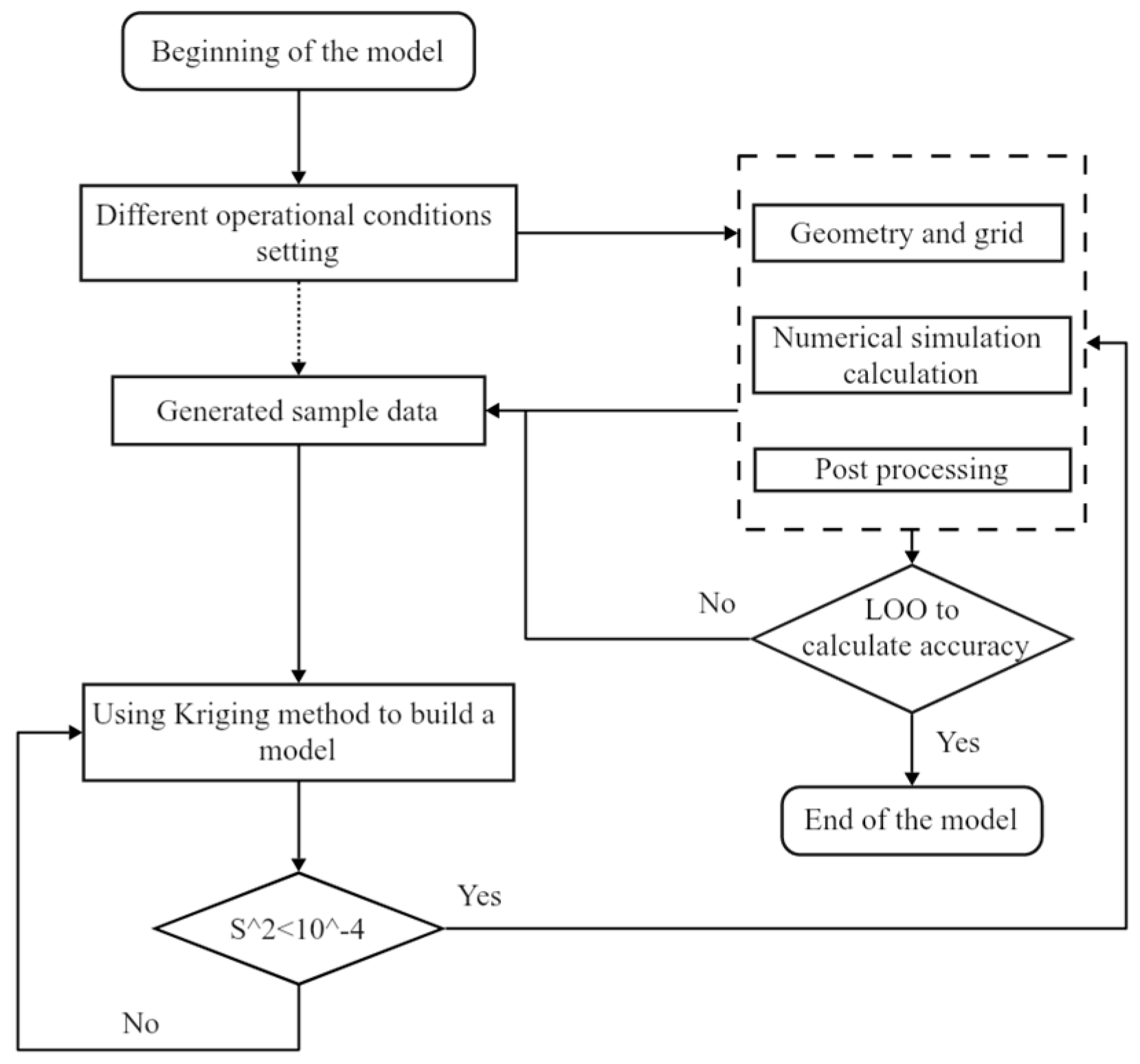
4. The Process of the Kriging Surrogate Model

A model based on the Kriging interpolation method was developed to describe the evolution mechanisms of the flow distortions at the turbine outlet and the vortex structure in the diffuser under different operational conditions. The development process of the Kriging surrogate model for the coupled aerodynamic performance of the turbine and diffuser system is presented in Figure 12. Firstly, a database of the coupling flow field in the turbine and diffuser, as a function of the inlet total pressure, was obtained by running a set of CFD solvers. Then, the Kriging method was used to establish the relationship model between the inlet aerodynamic parameters and the flow field characteristics of the coupled system. Finally, the distributions of the key aerodynamic parameters under any operational conditions are quickly calculated by the surrogate model. The accuracy of the Kriging model’s prediction results is verified using the leave-one-out method (LOO).

By referring to the setting method in Section 2.2, a database of the coupled flow field in the turbine and diffuser, as a function of the total pressure at the inlet, is generated by changing the inlet pressure. To obtain the database for the model, 15 sample points were selected between 140 kPa and 280 kPa using the Uniform Sampling method. By setting 15 groups of different inlet total pressure and total temperature conditions, denoted as S, the design space was established.

$$S=\left(\begin{array}{cc}{P}^1& T^1\\ P^2& T^2\\ \cdots & \cdots \\ P^n& T^n\end{array}\right)n\in (1,15)$$

(8)

The steady-state simulation is adopted to analyze the aerodynamic characteristics of the coupled system of the last-stage turbine and exhaust diffuser using CFD software. The corresponding response velocities $V={\{v^1,v^2,\cdots ,v^n\}}^T,n\in (1,15)$ are obtained from the complex numerical model simulations (in subsequent studies, velocity $V$ can be replaced by pressure P, flow angle θ, etc.). The sample dataset $(S,V_P)$ consists of all sample points and their corresponding responses.

The Kriging surrogate model assumes that all data are normally distributed in n dimensions. Then response velocities $V={\{v^1,v^2,\cdots ,v^n\}}^T,n\in (1,15)$, are given. Both $V$ and the input parameters satisfy the (0,1) Gaussian distribution.

$$V=\left[\begin{array}{ccc}\begin{array}{cc}{v}_1\left(S^1\right)& v_1\left(S^2\right)\\ v_2\left(S^1\right)& v_2\left(S^2\right)\end{array}& \cdots & \begin{array}{c}{v}_1\left(S^{15}\right)\\ v_2\left(S^{15}\right)\end{array}\\ ⋮& \ddots & ⋮\\ \begin{array}{cc}{v}_{15}\left(S^1\right)& v_{15}\left(S^2\right)\end{array}& \cdots & v_{15}\left(S^{15}\right)\end{array}\right]$$

(9)

The Kriging surrogate model estimates the value of the objective function $V_P$ as the sum of a linear polynomial trend model $\sum _{i=1}^p{\beta }_i{v}_i\left(s\right)$ and a systematic departure $z\left(s\right)$ representing low and high frequency variations around the trend model. The regression function is assumed to be a multivariate polynomial of the form.

$$\widehat{v}\left(s\right)={\sum }_{i=1}^p{\beta }_i{v}_i\left(s\right)+z\left(s\right)=\left[v_1\left(s\right),v_p\left(s\right)\right]\beta +z\left(s\right)={v_p\left(s\right)}^T\beta +z\left(s\right)$$

(10)

${\beta }_i={\beta }_0+{\beta }_{1}v+{\beta }_2{v}^2+\dots$, is the global trend term, and a polynomial trend is selected in this study. $v_i\left(x\right)$ denotes the basis functions.

$z\left(s\right)$ is a zero-mean Gaussian stochastic process with a mean is 0. Its spatial covariance is specified by Equation (11), which uses the Matérn function.

$$cov\left[z\left(s_i\right),z\left(s_j\right)\right]={\sigma }^{2}R(z\left(s_i\right),z\left(s_j\right)).$$

(11)

here, ${\sigma }^2$ is the process variance, $R$ represents the spatial correlation. In particular, for the Kriging surrogate model shown in Equation (12), the construction of $\mathit{R}$ selects Matérn functions.

$$\mathit{R}(s_i,s_j,l,\alpha )={\sigma }^2{\displaystyle \frac{2^{1-\alpha }}{\Gamma \left(\alpha \right)}}{\left(2\sqrt{\alpha }{\displaystyle \frac{|s_i-s_j|}{l}}\right)}^{\alpha }{\mathrm{K}}_{\alpha }\left(2\sqrt{\alpha }{\displaystyle \frac{|s_i-s_j|}{l}}\right)$$

(12)

where Matérn functions with shape parameter $\alpha =3/2$ and $\alpha =5/2$, known as Matérn-3/2 and Matérn-5/2, respectively. $l$ is the length-scale parameter, and its initial value is set to 0.01, which affects the rate of decay of spatial correlation.

The purpose of the Kriging surrogate model is to represent the function value of a position point by a weighted sum of the function values of sample points. The corresponding response of the sample points is used to predict the corresponding response of unknown points using the following model:

$$\widehat{v}\left(S\right)=c^{T}v$$

(13)

Then, the corresponding response of any design point in the design space can be estimated, given a suitable coefficient $c^T$. To obtain the correct coefficient, the error needs to be calculated using Equation (14).

$$\widehat{v}\left(s\right)-v\left(s\right)=c^{T}v-v\left(s\right)=c^T\left(V\beta +Z\right)-{v_p\left(s\right)}^T\beta +z\left(s\right)=c^{T}Z-z+{(V^{T}c-v(s\left)\right)}^T\beta$$

(14)

where $Z={\{z^1,z^2,\cdots ,z^n\}}^T,n\in 15$ represents the error at the sample points; z is the error at the unknown and sample point; and $V^{T}c$ is the basis function for the unknown points given by the weighted sum of the sample points, so it should be equal to the basis function for the unknown points, namely:

$$V^{T}c\left(s\right)=v\left(s\right)$$

(15)

Next, based on the above assumptions, the Kriging model seeks the optimal weighting coefficient $c$. The mean square error (MSE) is predicted to be the following:

$$MSE=E\left(\widehat{v}\left(s\right)-v\left(s\right)\right)=E\left[{\left(c^{T}Z-z\right)}^2\right]=E\left(z^2+c^{T}ZZc-2c^{T}Zz\right)={\sigma }^2(1+c^{T}Rc-2c^{T}r)$$

(16)

The Lagrange multiplier is constructed using the MSE and the equality constraint:

$$L\left(c,\lambda \right)={\sigma }^2\left(1+c^{T}Rc-2c^{T}r\right)-{\lambda }^T(V^{T}c-v)$$

(17)

$${\displaystyle \frac{\partial L}{\partial c}}=2{\sigma }^2\left(Rc-r\right)-V\lambda$$

(18)

The following matrix equation can be calculated:

$$\left[\begin{array}{cc}\mathit{R}& V\\ V^T& 0\end{array}\right]\left[\begin{array}{c}c\\ \widehat{\lambda }\end{array}\right]=\left[\begin{array}{c}\mathit{r}\\ v\end{array}\right]$$

(19)

where

$$\widehat{\lambda }=-{\displaystyle \frac{\lambda }{{2\sigma }^2}}$$

(20)

$$\mathit{R}=\left|\begin{array}{ccc}R\left(S^1,S^1\right)& \cdots & R\left(S^1,S^n\right)\\ ⋮& \ddots & ⋮\\ R\left(S^n,S^1\right)& \cdots & R\left(S^n,S^n\right)\end{array}\right|,n\in (1,15)$$

(21)

$$\mathit{r}=\left|{\displaystyle \genfrac{}{}{0pt}{}{R\left(S^1,S\right)}{\begin{array}{c}⋮\\ R(S^n,S)\end{array}}}\right|,n\in (1,15)$$

(22)

The covariance matrix of the sample points is $R_{ij}=R\left(\theta ,S_i,S_j\right),i,j=\mathrm{1,2},3,\cdots ,15$. The covariance matrix of the sample points and unknown points is then $r\left(x\right)={[R\left(\theta ,S_1,S\right),R\left(\theta ,S_2,S\right),\cdots ,R\left(\theta ,S_n,S\right)]}^{\mathrm{T}},n\in (1,15)$. θ represents the hyperparameters.

$$\mathit{R}=\left|\begin{array}{ccc}R\left(S^1,S^1\right)& \cdots & R\left(S^1,S^n\right)\\ ⋮& \ddots & ⋮\\ R\left(S^n,S^1\right)& \cdots & R\left(S^n,S^n\right)\end{array}\right|,n\in (1,15)$$

(23)

By solving Equation (18), the results can be obtained.

$$\widehat{\lambda }={{(V}^T{R}^{-1}V)}^{-1}{(V}^T{R}^{-1}r-v)$$

(24)

$$c=R^{-1}(r-V\widehat{\lambda })$$

(25)

By substituting Equations (22) and (23) into Equation (13), the expression for the equation can be obtained.

$$\widehat{v}\left(S\right)=R^{-1}\left(r-F\widehat{\lambda }\right)V_P={v\left(s\right)}^T{\beta }^{*}+{r\left(s\right)}^T{R}^{-1}\left(V_P-{\beta }^{*}F\right)$$

(26)

$${\beta }^{*}={{(V}^T{R}^{-1}V)}^{-1}{FV}^T{R}^{-1}{V}_P$$

(27)

$s^2$ and $\mathit{R}$ are the variance and correlation functions of the steady-state Gaussian process z(x), respectively. In addition, the mean square error estimated using the Kriging surrogate model can also obtained:

$$MSE\left(\widehat{v}\left(S\right)\right)=s^2\left(S\right)={\sigma }^2\left(1-r^T{R}^{-1}r+{\left(1-V^T{R}^{-1}r\right)}^2/{(V}^T{R}^{-1}V\right)$$

(28)

If $s^2\left(S\right)$ < ${\sigma }^{*}$(in this paper, ${\sigma }^{*}$ = ${10}^{-4}$), then the Kriging surrogate model converges well, $\widehat{v}\left(s\right)$ is the predicted value of the sample by the Kriging surrogate model.

If $s_{max}$ > $s^{*}$, then the learning function is used to select the next sample and add it to the sample set to update the training set S. The Kriging surrogate model is then rebuilt.

Due to the limited number of samples, leave-one-out (LOO) cross-validation is used to verify the calculation accuracy of the model. LOO not only verifies the rationality of the parameters l and α but also optimizes these parameters to improve the accuracy and generalization of the model. The original sample data are divided into a training sample set and a test sample set. The model is trained on the training sample set, and then the prediction error is evaluated on the test sample set. Multiple prediction errors can be obtained through multiple segmentations of the original sample data, and the cross-validation value (CV) of the prediction errors can be obtained after averaging. Finally, the minimum CV value is used as the basis for model selection. The error evaluation method of the leave-one-out method is as follows:

$$CV=\sqrt{{\displaystyle \frac{{\sum }_{i=1}^n{(v_i-{\widehat{v}}_{-i})}^2}{n}}}$$

(29)

where n is the number of validation points, and $v_i$ and ${\widehat{v}}_{-i}$ are the predicted and the actual values for each point.

5. The Reliability and Applications of the Model

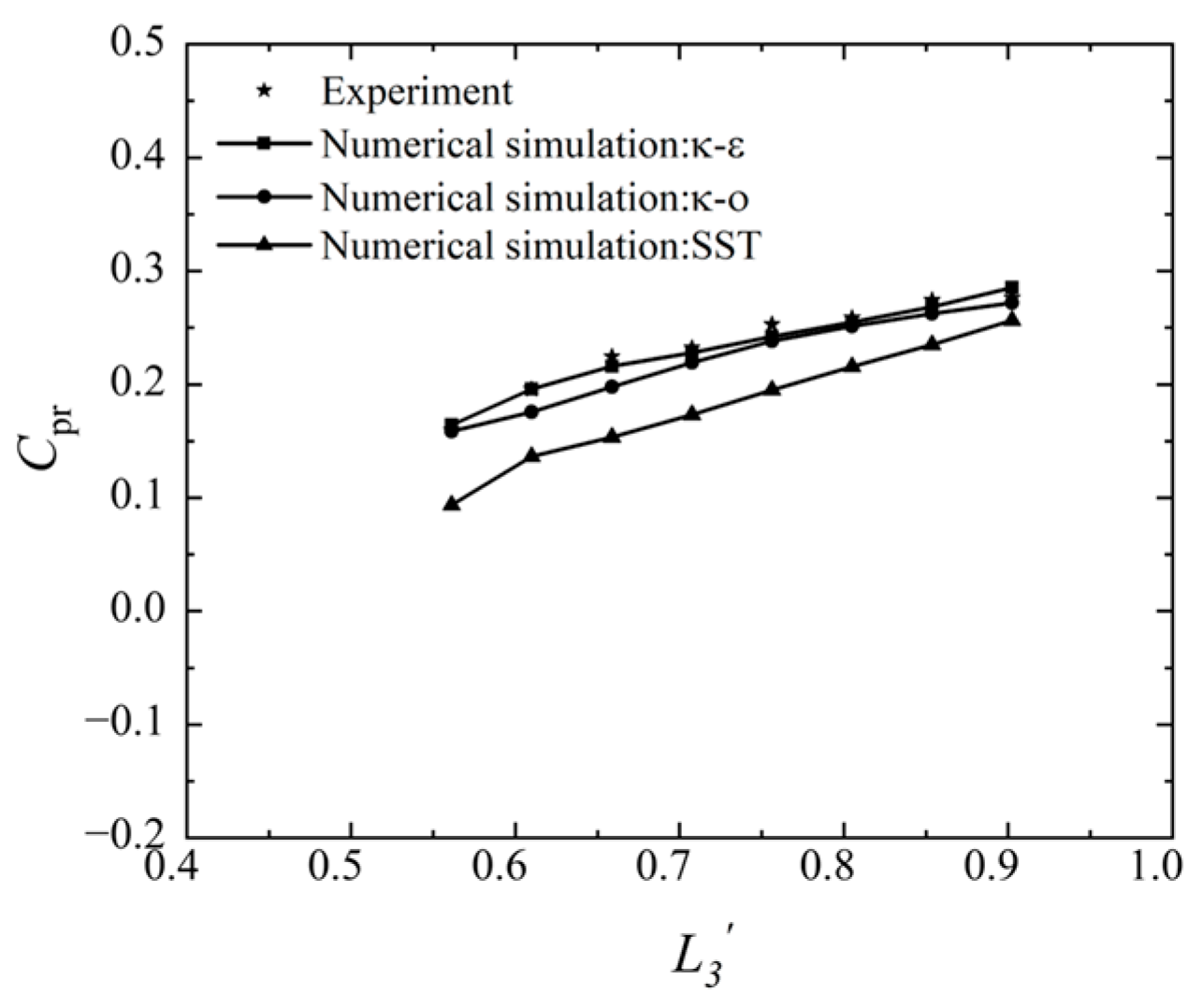
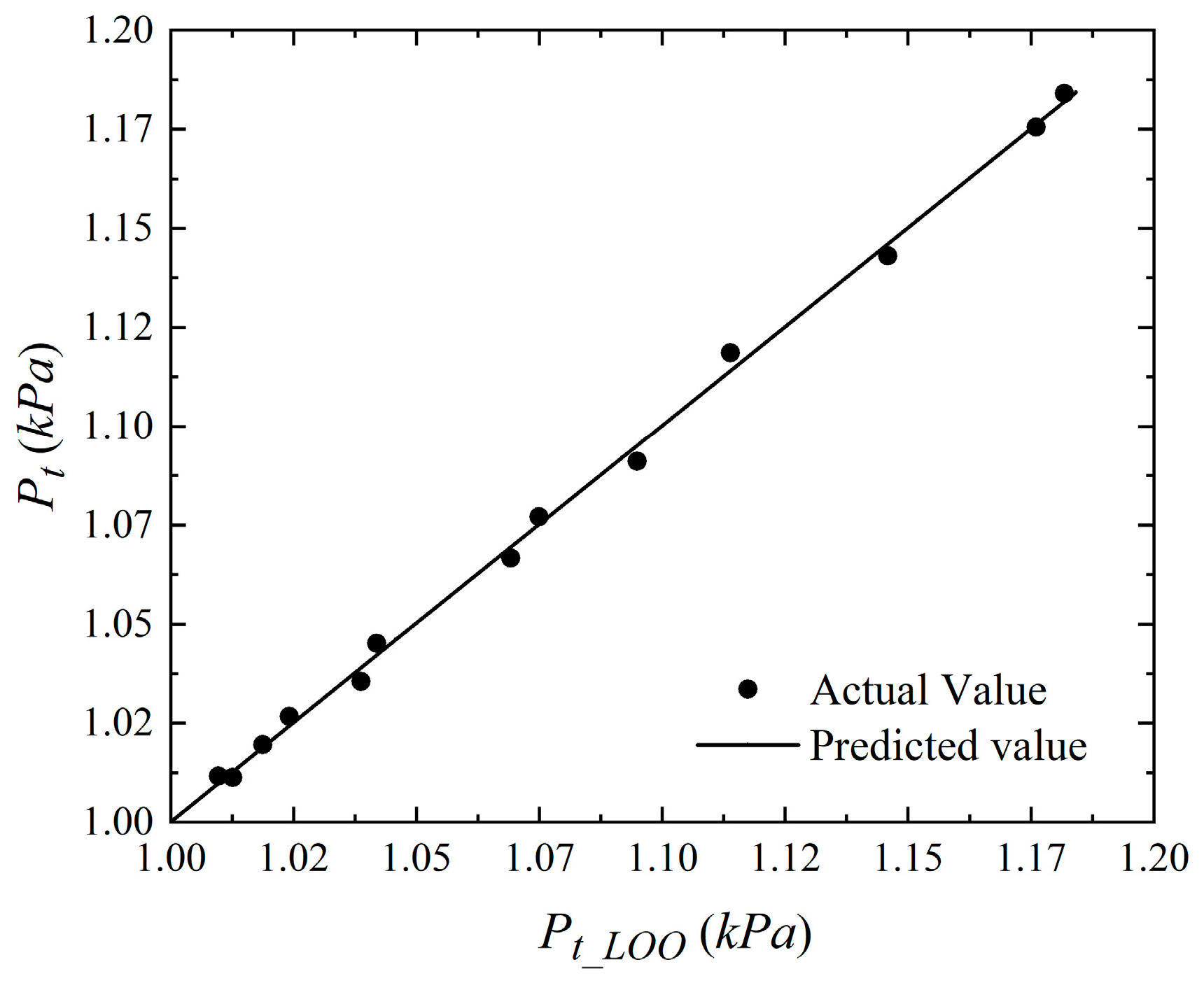
5.1. Accuracy Analysis

LOO is used to verify the accuracy of the Kriging surrogate model of the turbine and exhaust diffuser aerodynamic performance. It provides tools to calculate Kriging parameters for performing reliability or sensitivity analyses for each data point. To validate the overall behavior of each value, the CV error is used as an excellent general-purpose error metric for numerical predictions, as it amplifies and severely punishes large errors. CV errors between CFD simulation results and Kriging model prediction results were calculated; the minimum was 0.05%, and the average error was 0.35%, as shown in Figure 13. The Kriging model used in this paper has good generalization ability and high representativeness of the training set and can accurately predict the data.

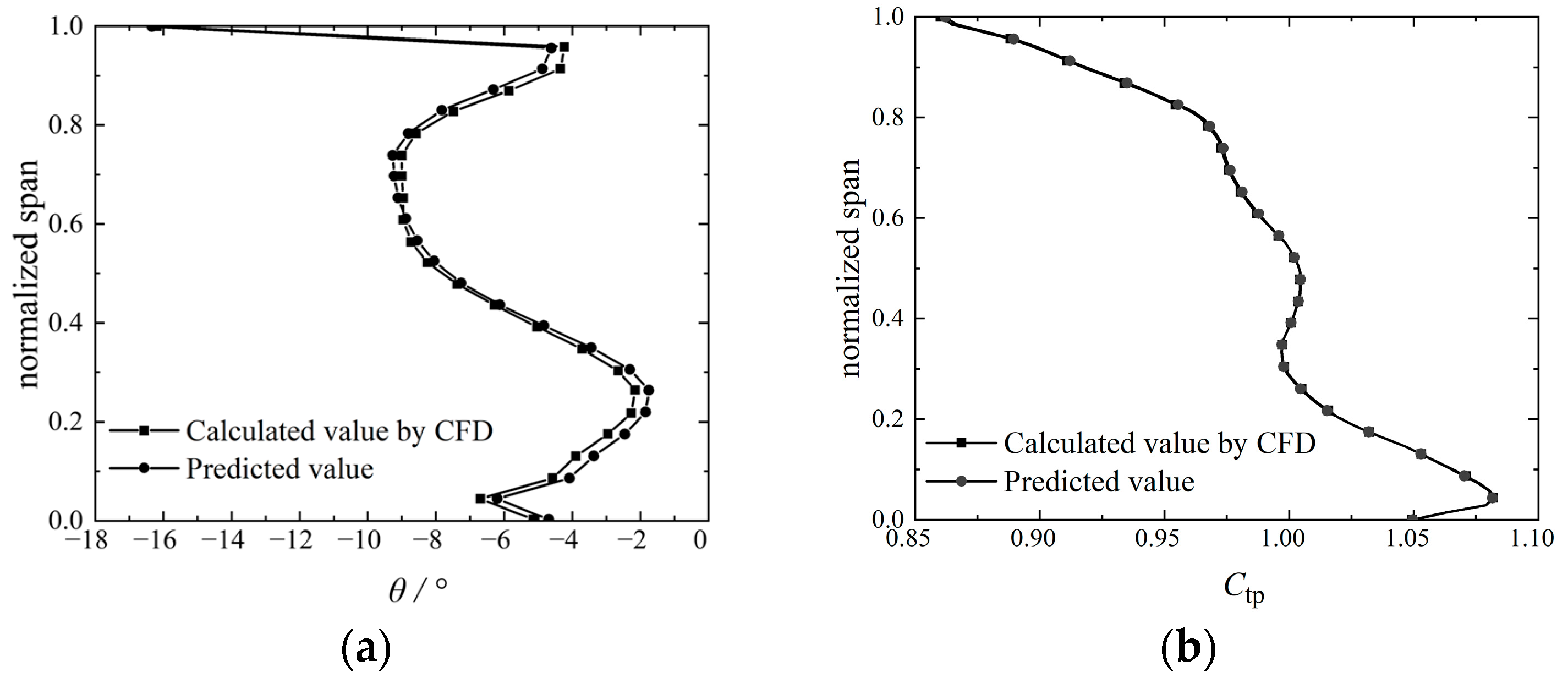
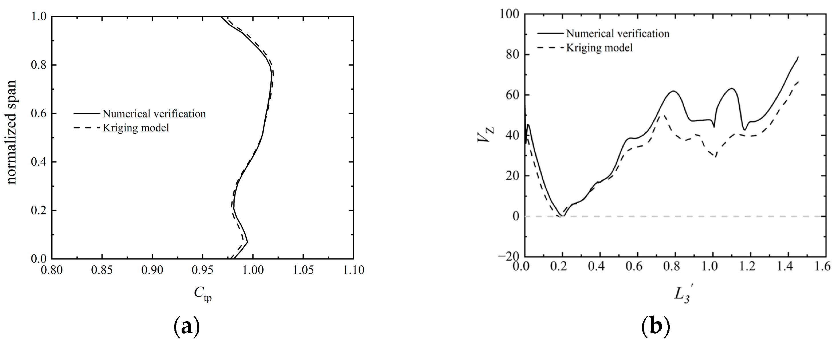
5.2. Comparison of Predicted Results

Given a specific inlet total pressure and total temperature, compared with numerical simulation, the prediction method based on the Kriging model can quickly obtain the radial distribution of the circumferential average total pressure and velocity at the turbine outlet, as shown in Figure 14. It can be seen that the prediction method can not only accurately predict the distribution trend of aerodynamic parameters on the section of the flow field but also achieve high accuracy in the prediction of values.

Furthermore, the model is used to predict the flow field in the coupled system. Figure 15 and Figure 16 show the prediction and simulation results of the turbine outlet axial Mach number (Ma) and the circumferential distribution of the total pressure coefficient under specific inlet conditions. Even in the prediction of complex two-dimensional flow fields, the model can calculate the flow field details at the sections of interest. The model can accurately obtain the circumferential and radial changes of the Mach number and total pressure at the diffuser inlet section. Even in the prediction of the complex two-dimensional flow field, the model can restore most of the detailed features of the flow field at the section of interest.

Table 4. Error of numerical simulation and prediction results.

	The Circumference Is Uniform		The Circumference Is Not Uniform
	Swirl Angle	Ctp	Ma	Ctp
Error	max/min/ave (%)	max/min/ave (%)	max/min/ave (%)	max/min/ave (%)
	18.81/0.84/7.23	0.23/0.01/0.06	15.3/0.18/7.45	3.8/0.78/1.98

shows the errors in the prediction results and the numerical simulation results. Here, max represents the maximum error, min represents the minimum error, and ave represents the average error. In the figure, the prediction effect of the single radial parameter distribution is compared with that of the flow field plane parameter. For the prediction of radial two-dimensional parameters, the maximum error in the axial Ma_z prediction is 18.81%, the minimum error is 0.84%, and the average error is 7.23%. The normalized total pressure prediction results are better, with errors less than 0.5%. For the axial Mach number prediction, the maximum error is 15.3%, the minimum error is 0.18%, and the mean error is 7.45%. The pressure prediction error ranges from 0.78% to 3.8%, with a mean value of 1.98%. Although there are some differences between multiple tests, the predicted results are in good agreement with the CFD simulation results both in flow pattern and numerical value. More sample data will reduce the accuracy, and this method is more accurate in predicting radial two-dimensional parameters.

Overall, the proposed surrogate model can accurately predict the averaged profiles of the aerodynamic parameters and 2D flow field at any section of interest in the coupled system.

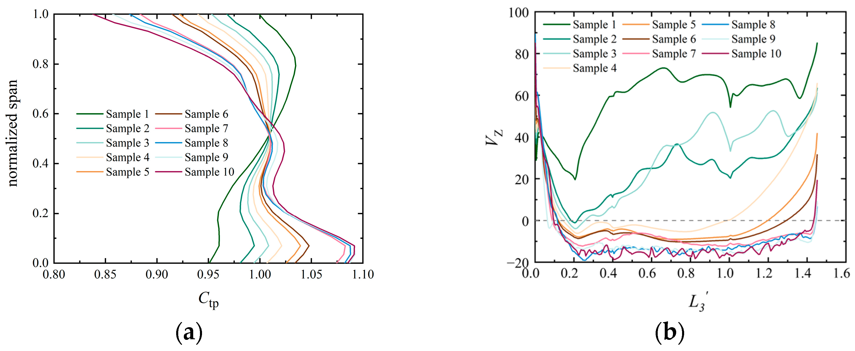
5.3. Application of the Kriging Surrogate Model to Describe the Flow Interaction Between Turbine and Exhaust Diffuser

As can be seen from Figure 15 and Figure 16, the flow field at the outlet of the annular diffuser is distributed in a clear and uniform radial direction. Therefore, the velocity distribution along the casing wall at any circumferential position was selected to characterize the separation vortex of the casing, as shown in Figure 17.

Ten operational points were selected from the sample points. The inlet total pressure and its corresponding wall velocity distribution were chosen as sample points, as shown in Figure 18. From the existing sample data, it can be observed that as the negative gradient of the total pressure near the casing at the inlet increases, the axial range of the separated vortex nearing the casing gradually expands. This also leads to a gradual increase in the intensity of the separated vortex. The greater the negative gradient of the total pressure, the weaker the capability to resist the adverse pressure gradient at the casing, leading to the separation point of the vortex moving closer to the inlet. Therefore, there must be a certain total pressure gradient that can trigger the separation vortex at the casing of the diffuser.

The axial velocity at the diffuser casing where the separation vortex begins to appear, as identified by the Kriging model, is shown in Figure 19a. Figure 19b presents the corresponding total pressure at the inlet. It can be observed that when the gradient of the total pressure coefficient at the inlet of the diffuser has a slope k = −4.37, as shown in Figure 19b, the separation vortex at the diffuser casing begins to emerge. The initial appearance of the separation vortex occurs at $L_3^{\prime }$ = 0.2, which corresponds to the juncture of the casing wall inside the annular diffuser.

6. Conclusions

In this paper, by studying the coupling flow field and aerodynamic performance of the last-stage turbine and exhaust diffuser under different conditions using CFD, the following conclusions are drawn.

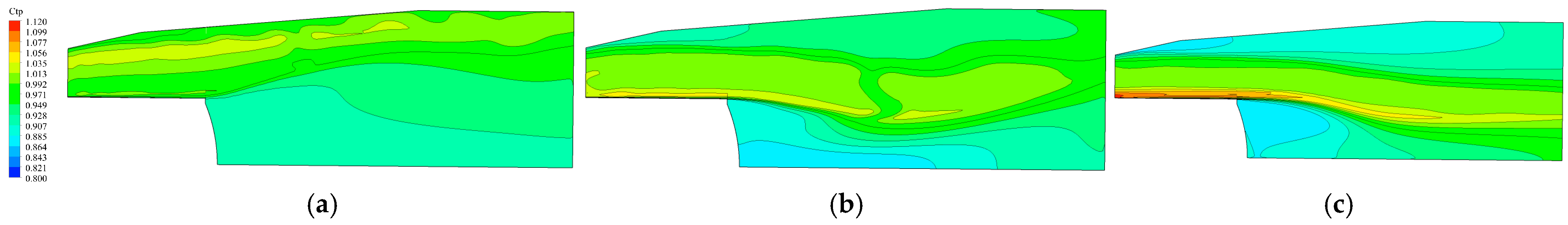
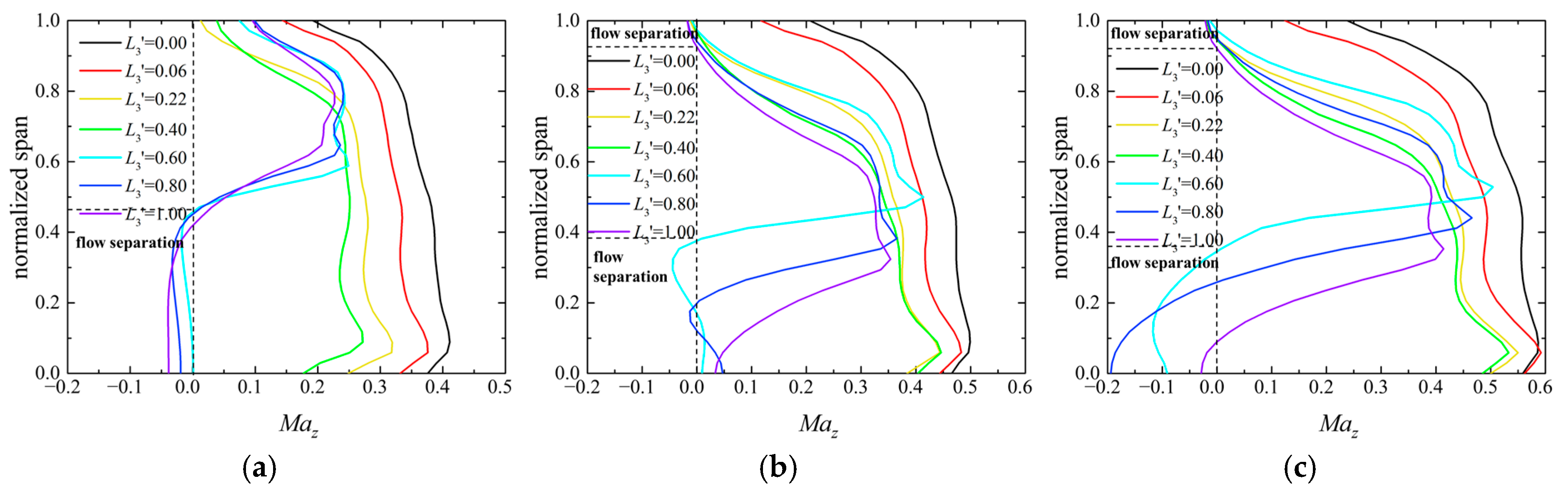
• The differences in the aerodynamic performance of the coupled turbine–diffuser system under various operational conditions are primarily attributed to the flow structure in the annular diffuser and the conical diffuser. The radial distribution profiles of total pressure and the axial velocity values are identified as the two key factors influencing the flow field evolution with changing operational conditions.
• A radial negative gradient in the total pressure at the turbine outlet tends to induce flow separation near the outer end-wall of the diffuser, thereby reducing the pressure recovery capacity. The axial velocity at the turbine outlet hub directly influences the strength of the backflow vortex in the conical diffuser, which in turn affects the total pressure loss. Quantitatively, the slope of the total pressure change along the blade height near the casing is k = −4.37, indicating a significant pressure drop that correlates with flow separation and vortex formation.
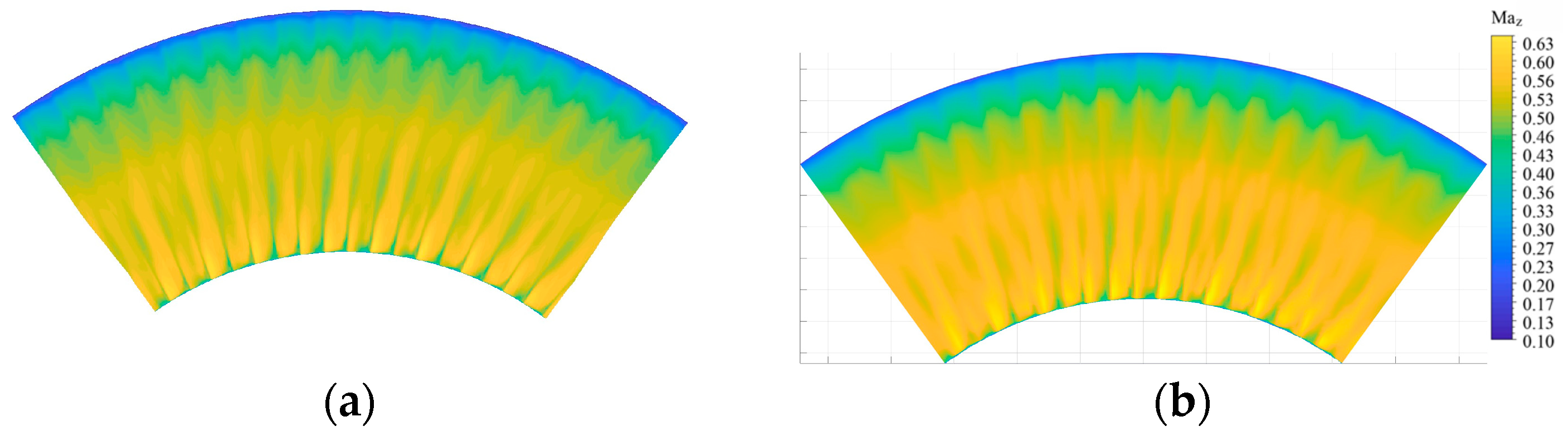
• A surrogate model was developed using a database generated by running a CFD solver and employing the Kriging interpolation method. This model provides a quantitative description of the relationships between operational conditions and key flow field characteristics in the coupled system. For the prediction of radial two-dimensional parameters, the maximum error of the axial Mach number (Ma_z) prediction is 18.81%, the minimum error is 0.84%, and the average error is 7.23%. The normalized total pressure prediction is more accurate, with an error of less than 0.5%. Additionally, the maximum error in the axial Mach number prediction is 15.3%, the minimum error is 0.18%, and the average error is 7.45%. The total pressure prediction error ranges from 0.78% to 3.8%, with an average error of 1.98%. The time consumed by the proposed surrogate model is much shorter than that of the CFD solver.
• The Kriging surrogate model presented in this paper uses Matérn functions to describe data with varying smoothness within a single model, which can better capture complex spatial correlation structures. The remaining method can reoptimize the hyperparameters and further improve the accuracy of the model. In the future, neural networks with more powerful nonlinear modeling capabilities will be added to further improve and deepen this area of research, and the methodology will be extended to other turbomachinery applications.

References

1. Kumar, D.S.; Kumar, K.L. Effect of swirl on pressure recovery in annular diffusers. J. Mech. Eng. Sci. 1980, 22, 305–313. [Google Scholar] [CrossRef]
2. Babu, M.; Bhatia, D.; Shukla, R.K.; Pradeep, A.M.; Roy, B. Effect of turbine tip leakage flows on exhaust diffuser performance. In Proceedings of the ASME 2011 Turbo Expo: Turbine Technical Conference and Exposition, Vancouver, BC, Canada, 6–10 June 2011. [Google Scholar]
3. Babu, M.; Shukla, R.K.; Maru, A.; Pradeep, A.M.; Roy, B. Boundary layer control in turbine exhaust diffusers using casing injection and design modifications. In Proceedings of the ASME Turbo Expo 2012: Turbine Technical Conference and Exposition, Copenhagen, Denmark, 11–15 June 2012. [Google Scholar]
4. Zimmermann, C.; Stetter, H. Experimental determination of the flow field in the tip region of a LP steam turbine. In Proceedings of the ASME 1993 International Gas Turbine and Aeroengine Congress and Exposition, Cincinnati, OH, USA, 24–27 May 1993. [Google Scholar]
5. Vassiliev, V.; Irmisch, S.; Abdel-Wahab, S.; Granovskiy, A. Impact of the inflow conditions on the heavy-duty gas turbine exhaust diffuser performance. In Proceedings of the ASME Turbo Expo 2010: Power for Land, Sea, and Air, Glasgow, UK, 14–18 June 2010. [Google Scholar]
6. Kluß, D.; Wiedermann, A.; Volgmann, W. Impact of gas turbine outflow on diffuser performance—A numerical study. In Proceedings of the ASME Turbo Expo 2004: Power for Land, Sea, and Air, Vienna, Austria, 14–17 June 2004. [Google Scholar]
7. Kuschel, M.; Drechsel, B.; Kluß, D.; Seume, J.R. Influence of turbulent flow characteristics and coherent vortices on the pressure recovery of annular diffusers: Part A—Experimental results. In Proceedings of the ASME Turbo Expo 2015: Turbine Technical Conference and Exposition, Montreal, QC, Canada, 15–19 June 2015. [Google Scholar]
8. Drechsel, B.; Müller, C.; Herbst, F.; Seume, J.R. Influence of turbulent flow characteristics and coherent vortices on the pressure recovery of annular diffusers: Part B—Scale-resolving simulations. In Proceedings of the ASME Turbo Expo 2015: Turbine Technical Conference and Exposition, Montreal, QC, Canada, 15–19 June 2015. [Google Scholar]
9. Steven, S.J.; Williams, Q.J. The influence of inlet conditions on the performance of annular diffusers. J. Fluids Eng. 1980, 102, 357–363. [Google Scholar] [CrossRef]
10. Vassiliev, V.; Irmisch, S.; Florjancic, S. CFD analysis of industrial gas turbine exhaust diffusers. In Proceedings of the ASME Turbo Expo 2002: Power for Land, Sea, and Air, Amsterdam, The Netherlands, 3–6 June 2002. [Google Scholar]
11. Vassiliev, V.; Irmisch, S.; Claridge, M.; Richardson, D.P. Experimental and numerical investigation of the impact of swirl on the performance of industrial gas turbines exhaust diffusers. In Proceedings of the ASME Turbo Expo 2003, Collocated with the 2003 International Joint Power Generation Conference, Atlanta, GA, USA, 16–19 June 2003. [Google Scholar]
12. Tsoutsanis, E.; Meskin, N. Derivative-driven window-based regression method for gas turbine performance prognostics. Energy 2017, 128, 302–311. [Google Scholar] [CrossRef]
13. Huang, Z.; Wang, C.; Chen, J.; Tian, H. Optimal design of aeroengine turbine disc based on kriging surrogate models. Comput. Struct. 2011, 89, 27–37. [Google Scholar] [CrossRef]
14. Wang, H.; Zhu, X.; Du, Z. Aerodynamic optimization for low pressure turbine exhaust hood using kriging surrogate model. Int. Commun. Heat Mass Transf. 2010, 37, 998–1003. [Google Scholar] [CrossRef]
Figure 1. Computational domain model of the full-scale gas turbine model.
Energies 18 00921 g001
Figure 2. Computational mesh.
Energies 18 00921 g002
Figure 3. Independence verification of computational mesh.
Energies 18 00921 g003
Figure 4. Test facility.
Energies 18 00921 g004
Figure 5. Pressure recovery coefficient axial distributions.
Energies 18 00921 g005
Figure 6. Total pressure coefficient and streamlines at turbine outlet (Section 2): (a) Case 1, (b) Case 2, (c) Case 3.
Energies 18 00921 g006
Figure 7. Flow field at the turbine stage outlet: (a) axial Mach number, (b) absolute tangential flow angle, (c) total pressure coefficient.
Energies 18 00921 g007
Figure 8. Comparison of diffuser performance under different operational conditions: (a) static pressure recovery loss coefficient, (b) total pressure loss coefficient.
Energies 18 00921 g008
Figure 9. Total pressure coefficient contour at section θ = 0° in the diffuser under different operational conditions: (a) Case 1, (b) Case 2, (c) Case 3.
Energies 18 00921 g009
Figure 10. Pressure coefficient contour and 2D streamline at section θ = 0° in the diffuser under different operational conditions: (a) Case 1, (b) Case 2, (c) Case 3.
Energies 18 00921 g010
Figure 11. Radial distributions of circumferential averaged Mach number at different axial positions in the diffuser: (a) Case 1, (b) Case 2, (c) Case 3.
Energies 18 00921 g011
Figure 12. The process of coupling model based on the Kriging model.
Energies 18 00921 g012
Figure 13. Comparison of the error of the leave-one-out method.
Energies 18 00921 g013
Figure 14. Prediction results of swirl angle and total pressure of the turbine outlet: (a) swirl angle, (b) total pressure.
Energies 18 00921 g014
Figure 15. Comparison of axial Ma number contours calculated by Kriging surrogate model and CFD solver: (a) Calculated by CFD solver (b) Calculated by surrogate model.
Energies 18 00921 g015
Figure 16. Comparison of total pressure contours calculated by Kriging surrogate model and CFD solver: (a) Calculated using a CFD solver. (b) Calculated using a surrogate model.
Energies 18 00921 g016
Figure 17. The circumferential position of static pressure points of the casing.
Energies 18 00921 g017
Figure 18. Sample point: (a) inlet total pressure distribution, (b) wall velocity distribution at the casing along the flow direction.
Energies 18 00921 g018
Figure 19. Initial condition of separation vortex: (a) inlet total pressure distribution, (b) wall velocity distribution at the casing.
Energies 18 00921 g019