Research on Export Oil and Gas Concentration Prediction Based on Machine Learning Methods

Abstract

With the oil industry’s increasing focus on environmental protection and the growing implementation of oil and gas recovery devices in depots, it is crucial to investigate the outlet concentrations of oil and gas from these devices. This research aims to reduce energy consumption while enhancing the efficiency of oil and gas recovery processes. This paper investigates the prediction of outlet oil and gas concentration based on the process parameters of oil and gas recovery devices in oil depots. This study employs both regression and classification machine learning models. Most regression models achieve a goodness-of-fit of approximately 0.9 and an accuracy error of about 30%. Additionally, most classification models attain over 90% accuracy, with predictions of high oil and gas concentrations reaching up to 84.5% accuracy. Both models demonstrate that the Random Forest method is more effective in predicting the exported oil and gas concentration with multiple-parameter inputs, providing a relevant basis for subsequent control of exported oil and gas concentration.

1. Introduction

In recent years, the petroleum industry has increasingly focused on environmental protection issues. Consequently, domestic petrochemical emissions are subjected to more stringent reviews, environmental standards have become more refined [1] to address the issue of excessive emissions in the petrochemical industry, and oil and gas recovery devices have been gradually implemented in the oil and gas sector. To tackle this problem in petrochemical depots, oil and gas recovery technologies are being progressively adopted; however, their specific applications vary across different depot environments. Currently, the main oil and gas recovery technologies used are the absorption, adsorption [2,3], condensation [4,5] and membrane separation methods [6]. The absorption method is based on the principle of using a specialized absorbent to promote the dissolution of one or more gas components while retaining other constituents in the air, thus achieving effective separation. In previous studies, the main focus has been on the selection of absorbents. Roizard et al. utilized osmotic evaporation as a method for absorbent recycling and examined the energy requirements for solvent regeneration during the osmotic evaporation process [7]. Regarding the selection of the absorbent material, Chiang et al. chose to use silicone oil, a hydrophobic absorbent, to separate volatile organic compounds (VOCs) and toluene from oil and gas [8]. The adsorption method, as a conventional separation technique, has extensive applications in oil and gas recovery systems. Its key technology is based on the careful selection of adsorbent materials and desorption methods [9,10]. The condensation method utilizes a refrigeration system to facilitate the liquefaction of non-methane hydrocarbons present in the gas, with the aim of achieving their subsequent separation [11,12]. The key technological aspect lies in the careful selection of adsorption materials and desorption methods. In the field of membrane separation technology, which is a relatively novel approach to separation, it is essential not only to prioritize the selectivity and permeability of the membrane but also to evaluate its resistance to potential erosion caused by oil vapors [11]. The four methods display unique characteristics. Throughout the development process, targeted optimization of the oil and gas recovery device is essential to address practical challenges encountered. As a result, the implementation of multi-combination and multi-stage oil and gas recovery systems has become the dominant trend in China.

In the research on predicting the concentration of oil and gas emissions, there has been a predominant focus on investigating the impact of individual variables, such as inlet flow rates and temperatures of oil and gas, on the resulting concentrations at the outlet. Insufficient research has been conducted on the impact of multivariate variables on outlet oil and gas concentrations, making it challenging to establish correlations between parameters due to the presence of numerous devices in the oil and gas recovery system. Moreover, the complexity of process parameters further obscures their interrelationships. In recent years, the application of machine learning in the petrochemical industry has gained significant attention due to its capability to effectively handle large-scale complex datasets and uncover intricate data correlations [13,14]. Wang et al. used BP Neural Networks to predict the effectiveness of heavy oil recovery, and the results indicated that BP Neural Networks are viable for predicting heavy oil recovery [15]. Liu et al. employed a machine learning approach to predict ethane recovery in a lean gas ethane recovery process; their support vector regression model, enhanced by grey wolf optimization, yielded the highest prediction accuracy [16]. Orru et al. used Support Vector Machines and multilayer perceptrons to identify and predict centrifugal pump failures in the oil and gas industry [17]. Yue et al. employed three machine learning methods to investigate the effects of reservoir parameters, horizontal well parameters, and injection parameters on CO₂ flood recovery, and developed a machine-learning-based recovery prediction model [18]. The study above clearly demonstrates that machine learning can effectively address relevant issues in the petrochemical industry. In particular, it can significantly improve the accuracy of various petrochemical prediction problems when provided with appropriate parameters [19,20]. This demonstrates the feasibility and value of exploring machine learning techniques for predicting the outlet oil and gas concentrations in oil and gas recovery devices.

However, according to the latest survey, in order to improve the transportation efficiency and reduce safety risks in the petrochemical industry, many machine learning methods have been adopted to solve the prediction problem, and different prediction problems have different algorithm models. Most of them try to select a more suitable model by comparing different algorithms [21,22]. Therefore, this study employs a diverse range of machine learning algorithms to predict the outlet oil and gas concentration in the oil and gas recovery system using on-site process parameters obtained from the oil depot’s recovery device. The aim is to assist the oil depot in optimizing process parameters to reduce costs and enhance efficiency.

2. Model Basis

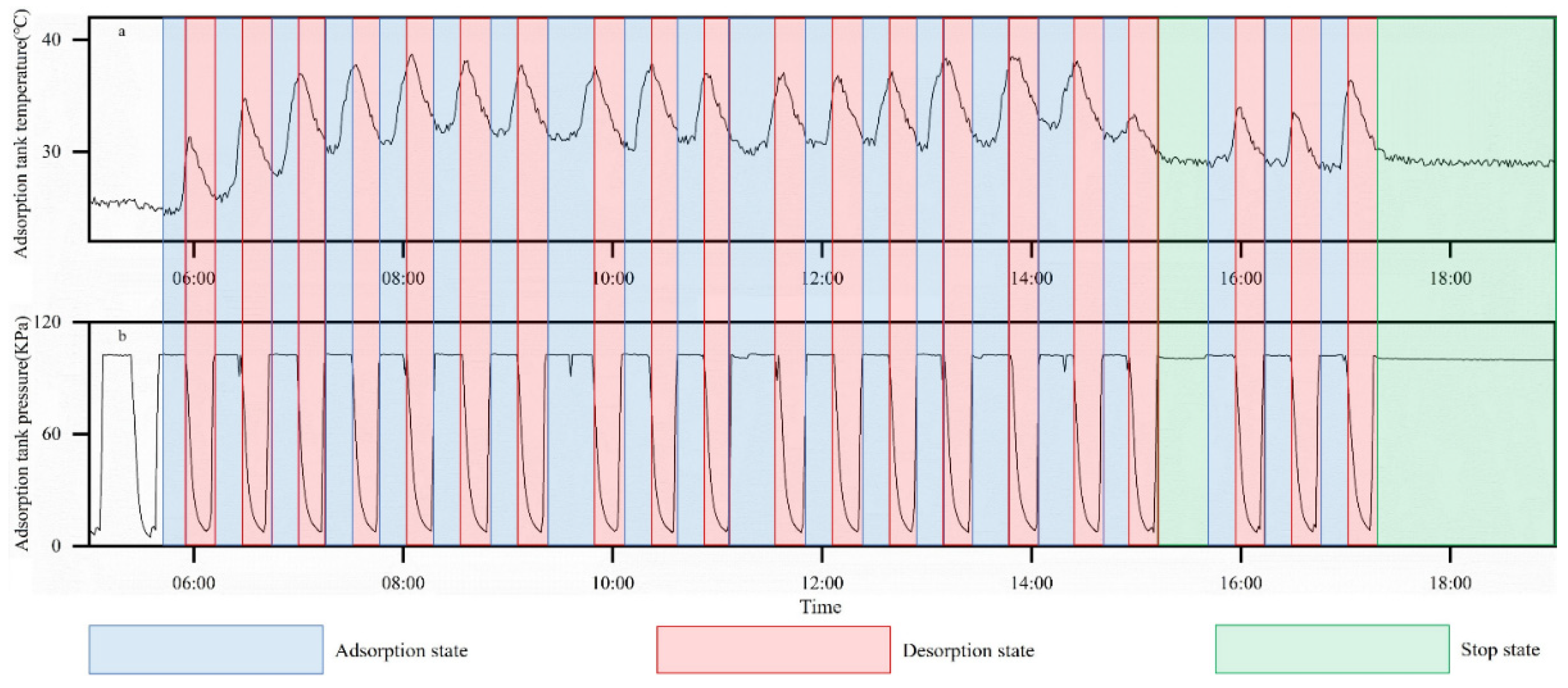
2.1. Process Flow Analysis

The oil and gas recovery device investigated in this study is based on the equipment utilized in an oil depot. The device employs a process that combines low-temperature absorption, high-efficiency agglomeration, and graded adsorption, integrating both absorption and adsorption methods. Additionally, an agglomerator is incorporated between the absorption tower and the adsorption tower. The flow chart of the oil and gas recovery device at the oil depot is illustrated in Figure 1. The process parameters provided by the device instrumentation include inlet oil and gas temperature (T101), inlet oil and gas flow (FI101), inlet oil and gas concentration (AT101), inlet oil and gas pressure (PI101), outlet temperature of the refrigeration unit (TT301), compressor outlet temperature (TI201A, TI201B), and carbon bed temperatures in two adsorption tanks (TI121, TI131).

The temperature and pressure data from each node in this device are directly obtained from the instrument, ensuring enhanced accuracy and precision. The concentration and flow rate of the inlet oil and gas are processed using instrumentation and signal conversion techniques to account for scale conversion and ensure safe device operation. The crane pipe signal serves as the start/stop signal during operation to ensure operational safety and prevent device malfunction caused by insufficient actual inlet oil/gas flow rate. To convert the inlet oil/gas flow rate accurately, it is multiplied by a factor of 118.2 m³ h⁻¹ based on the magnitude of the crane pipe signal.

The unit of the inlet oil and gas concentration is vol%, which differs from the unit of the outlet oil and gas concentration, mg m⁻³, necessitating conversion; Equations (1) and (2) serve as the conversion formulas between the two scales.

$$1\%Vol=10000 ppm$$

(1)

$${\displaystyle \frac{\mathrm{mg}}{{\mathrm{m}}^3}}={\displaystyle \frac{\mathrm{M}}{22.4}}\cdot \mathrm{ppm}\cdot \left[{\displaystyle \frac{273}{273+\mathrm{T}}}\right]\ast \left({\displaystyle \frac{\mathrm{Ba}}{101325}}\right)$$

(2)

where M is the relative molecular weight of the measured gas; 22.4 is the molecular weight of an ideal gas at 0 °C (273 K) and one standard atmospheric pressure in L/mol; ppm is the volume concentration value of the measured gas; T is the temperature in °C; and Ba is the pressure in Pa. Since the measurement environment is at 25 °C and standard atmospheric pressure, the uncertain quantities in the formula are the relative molecular weight M and the volume concentration value in ppm. The latter can be measured by the instrument, while the former will vary due to the different gas components. To facilitate conversion, this article sets the molecular weight of gasoline vapor at the outlet of the oil and gas recovery device as 45 in accordance with GB 20950-2007 [23] “Emission Standard of Air Pollutants for Oil Storage Depots”. The requirement for the concentration of emitted oil and gas is based on non-methane hydrocarbon (NMHC). Therefore, hereafter, NMHC and outlet oil and gas concentration refer to the same concept.

After completing the unit conversion, it is crucial to consider the variations in each parameter and the switching of adsorption tanks during operation. Since different adsorption tanks exhibit distinct adsorption effects, it is necessary to filter out the temperature of the adsorption tanks in the adsorption state while organizing the dataset and include it in the calculation model as an input variable.

2.2. Data Processing

After analyzing the process flow of oil and gas recovery, the input parameters considered in the prediction model include the inlet temperature, concentration, flow rate, and pressure of oil and gas; the outlet temperature of the refrigeration unit; the temperature of the adsorption tank; and the compressor outlet temperature. The prediction target is the outlet concentration of oil and gas. The parameter that requires special treatment is the temperature of the adsorption tank, which must be filtered based on the operational status of the tank. Generally, the operational state of the adsorption tank can be categorized into three distinct phases: adsorption, desorption, and cessation. As depicted in Figure 2, during the adsorption phase of the tank, the pressure within the adsorption tank closely approximates standard atmospheric pressure. Furthermore, as the adsorption process continues, there is a gradual increase in temperature within the tank. When the adsorption tank is in the desorption state, the pressure gradually decreases to 0 Kpa during compressor operation and returns to atmospheric pressure through a small valve upon completion of desorption. Simultaneously, the temperature of the charcoal bed in the adsorption tank gradually declines. When the temperature of the adsorption tank remains constant and the pressure is maintained at atmospheric levels, this indicates that the adsorption tank is in a state of cessation. Based on these operational characteristics, it can be inferred that by monitoring changes in pressure and temperature within the adsorption tank, we can classify its operational status.

After dividing the operating status of the adsorption tank and eliminating outliers, a total of 1379 data points were obtained.

Table 1. Selected data from the dataset and information about the data.

	Data 1	Data 2	Data 3	Data 4	Data 5	Data XXX
TI121 (°C)	31.95	36.21	35.32	35.47	33.91	34.49
PI101 (KPa)	−0.39	−0.75	−0.96	−0.39	−0.16	−0.36
AT101 (mg m−3)	150,651.00	150,712.00	150,638.00	150,675.00	150,602.00	150,663.00
TI101 (°C)	24.33	27.30	29.36	29.41	23.87	26.53
TI301 (°C)	23.85	23.59	23.86	23.64	24.07	23.69
TI201A (°C)	75.72	72.28	73.82	76.54	73.86	75.76
TI201B (°C)	71.84	67.02	69.2	72.98	66.22	70.28
FI101 (m3 h−1)	945.6	929.69	929.69	929.69	929.69	929.69
NMHC (mg m−3)	21,352.99	122,504.00	113,168.40	90,060.49	66,273.78	64,245.71

Note: T101 is inlet oil and gas temperature, FI101 is inlet oil and gas flow, AT101 is inlet oil and gas concentration, PI101 is inlet oil and gas pressure, TT301 is outlet temperature of the refrigeration unit, TI201A and TI201B present compressor outlet temperature, TI121 and TI131 present carbon bed temperatures in two adsorption tanks.

and

Table 2. Information about the data in the dataset.

	Maximum Values	Minimum Value	Average Value	(Statistics) Standard Deviation
TI121(°C)	39.84	22.85	30.99	3.06
PI101 (KPa)	1.44	−1.11	0.17	0.43
AT101 (mg m−3)	151,312.00	75,913.00	113,011.10	23,648.61
TI101 (°C)	36.52	19.52	25.23	3.49
TI301 (°C)	26.13	6.17	16.59	6.06
TI201A (°C)	80.16	31.00	66.63	9.72
TI201B (°C)	79.22	28.44	62.64	8.67
FI101 (m3 h−1)	1063.80	0.00	390.68	282.4685
NMHC (mg m−3)	146,168.10	201.09	9752.58	18,219.62

present comprehensive information on these data, including partial data, maximum and minimum values, mean values, and standard deviations for each parameter. The parameters with lower variability are TI121, TI101, TI301, TI201A, and TI201B, while those with higher variability are FI101, PI101, AT101, and non-methane hydrocarbon (NMHC). The data do not exhibit a linear relationship with one another.

3. Methodology

The machine learning algorithms utilized in this paper include BP Neural Networks, Support Vector Machines, Random Forests, BP Neural Networks based on the Particle Swarm Optimization Algorithm, Support Vector Machines based on the Particle Swarm Optimization Algorithm, and Genetic-Algorithm-Based BP Neural Network.

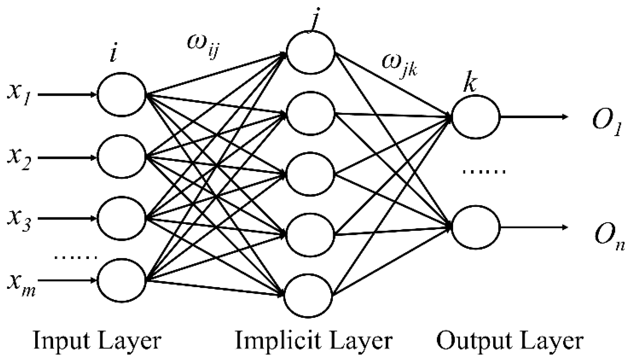
3.1. BP Neural Network

The BP Neural Network is a multi-layer feed-forward Neural Network commonly used in classification and regression problems. Its training process consists of two steps: forward propagation to compute the output and back propagation to calculate the gradient and update the weights. The primary principle of its operation is to update the weights and biases of the network using the back propagation algorithm to minimize the error between the predicted output and the true labels [24,25]. The following schematic diagrams and explanations are based on relevant research [26]. Consider a three-layer backpropagation Neural Network, as shown in Figure 3 below.

The output of the implicit layer is set to $F_j$. The input of the output layer is set as $O_k$, the excitation function of the system is set to be G, and the learning rate is set to be β; then, there is the following mathematical relationship between its three layers, where $a_j$ and $b_k$ represent the bias of the hidden layer and the output layer, respectively:

$$\left\{\begin{array}{c}{F}_j=G\left({\displaystyle \sum _{i=1}^m}{\omega }_{ij}{x}_i+a_j\right)\\ O_k={\displaystyle \sum _{j=1}^l}{F}_j{\omega }_{jk}+b_k\end{array}\right.$$

(3)

The desired output of the system is set as $T_k$. The error E of the system can be expressed by the variance between the actual output and the desired target value as follows:

$$E={\displaystyle \frac{1}{2}}\sum _{k=1}^n{(T_k-O_k)}^2$$

(4)

and let $e_k=T_k-O_k$ The system weights and biases are updated using the gradient descent principle as follows:

$$\begin{array}{c}\left\{\begin{array}{c}{\omega }_{ij}={\omega }_{ij}+\beta F_j(1-F_j)x_i{\displaystyle \sum _{k=1}^n}{\omega }_{jk}{e}_k\\ {\omega }_{jk}={\omega }_{jk}+\beta F_j{e}_k\end{array}\right.\\ \left\{\begin{array}{c}{a}_j=a_j+\beta F_j(1-F_j)x_i{\displaystyle \sum _{k=1}^n}{\omega }_{jk}{e}_{k_{\leftarrow }}\\ b_k=b_k+\beta e_k\end{array}\right.\end{array}$$

(5)

The BP Neural Network has a strong self-learning and self-adaptive ability and can handle a large amount of process parameter data of oil and gas recovery system. At the same time, in the BP Neural Network there is also easy overfitting and a local optimum, which is due to the algorithm’s high requirements for data preprocessing and the difficulty of tuning parameters. With the support of optimization algorithms, it can be more widely used in various projects.

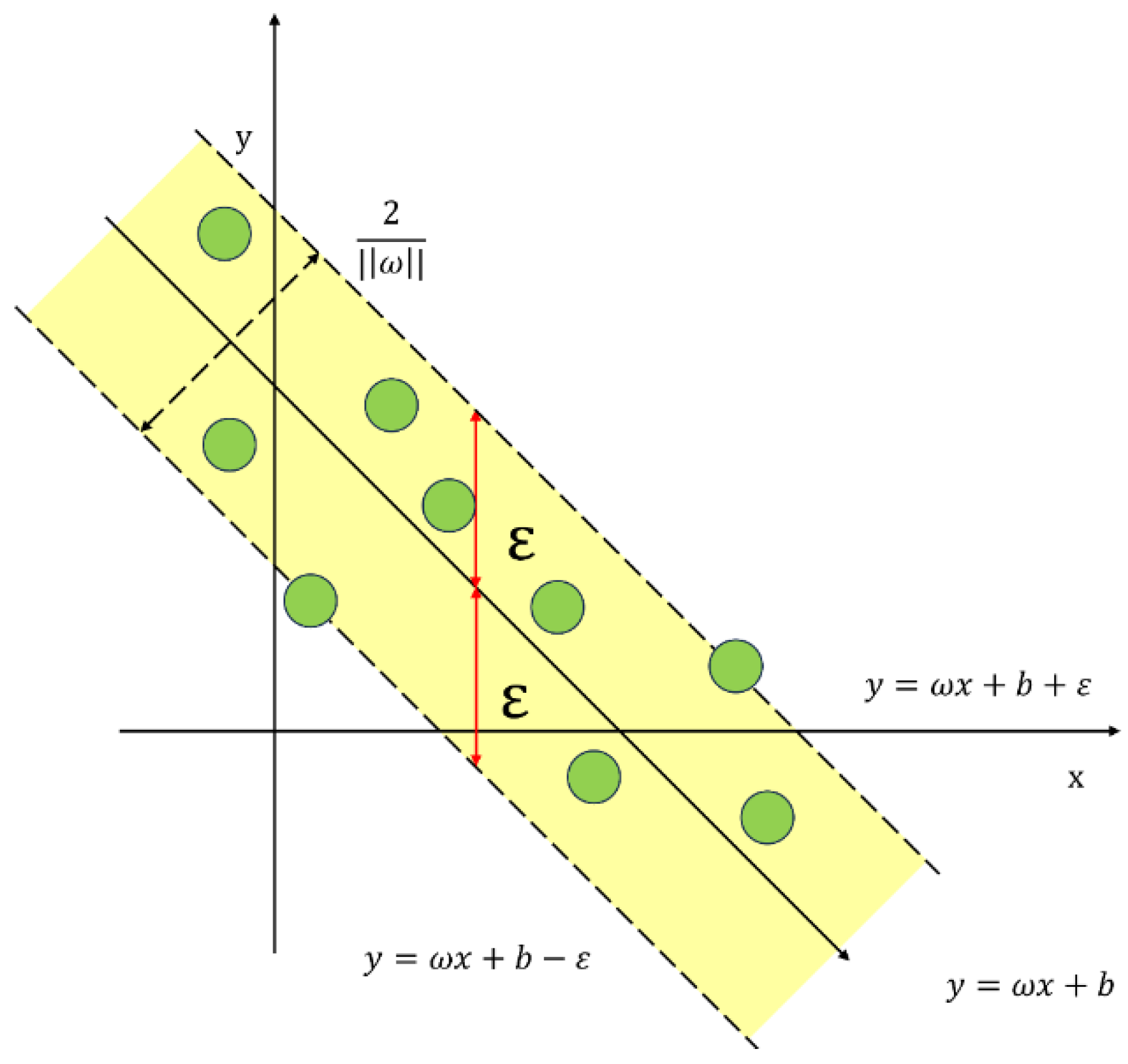
3.2. Support Vector Machines

An SVM is a supervised learning algorithm used for classification and regression. Its core idea is to separate data into different classes by selecting the best hyperplane. The goal of an SVM is to find an optimal hyperplane that can separate different classes of data. For linearly separable data, the hyperplane can be expressed as: w⋅x + b = 0. An SVM identifies the optimal hyperplane by maximizing the classification margin. The margin is defined as the distance from the nearest point to the hyperplane (called the support vector) to the hyperplane itself. During training, an SVM aims to maximize this margin while ensuring that all sample points are correctly classified, thereby providing the model with good generalization ability [27,28].

For a general regression problem, given training samples D = {(x1, y1),(x2, y2),…,(xn, yn)}, we wish to learn an f(x) that is as close as possible to y. w, b are the parameters to be determined. {(xn, yn)}, we wish to learn an f(x) that is as close as possible to y, with w, b being the parameters to be determined. In this model, the loss is zero only when f(x) is exactly the same as y. Support vector regression assumes that we can tolerate at most ε deviation between f(x) and y. The loss is computed when, and only when, the absolute value of the difference between f(x) and y is greater than ε. In this case, it is equivalent to constructing a spacer band of width 2ε centered on f(x), and if a training sample falls into the spacer band, it is deemed to be correctly predicted. Figure 4 illustrates the principle of the text above [29].

Thus, the SVR problem can be transformed into the following (the left part of the following equation is the regularization term):

$$\underset{w,b}{\min }{\displaystyle \frac{1}{2}}||w|{|}^2+C\sum _{i=1}^m{\mathcal{l}}_c(f(x_i)-y_i)$$

(6)

The left part of the above equation is the regularization term and the right part of the equation is the loss function:

$${\mathcal{l}}_{{\epsilon }_{ϵ}}(z)=\left\{\begin{array}{c}0, \mathrm{if}|z|⩽ϵ\hfill \\ |z|-ϵ, \mathrm{otherwise}\hfill \end{array}\right.$$

(7)

Thus, a relaxation factor is introduced, and the SVR problem is:

$$\begin{array}{c}\underset{w,b,{\xi }_i,{\widehat{\xi }}_i}{\min }{\displaystyle \frac{1}{2}}||w|{|}^2+C{\displaystyle \sum _{i=1}^m}\left({\xi }_i+{\widehat{\xi }}_i\right)\\ \mathrm{s}.\mathrm{t}.f(x_i)-y_i⩽ϵ+{\xi }_i,\\ y_i-f(x_i)⩽ϵ+{\widehat{\xi }}_i\\ {\xi }_i⩾0,{\xi }_i⩾0,i=1,2,\dots ,m.\end{array}$$

(8)

Finally, the introduction of Lagrange multipliers leads to the Lagrange function:

$$\begin{array}{c}L(w,b,\alpha ,\widehat{\alpha },\xi ,\widehat{\xi },\mu ,\widehat{\mu })\\ ={\displaystyle \frac{1}{2}}\Vert w {\Vert }^2+C{\displaystyle \sum _{i=1}^m}\left({\xi }_i+{\widehat{\xi }}_i\right)-{\displaystyle \sum _{i=1}^m}{\mu }_i{\xi }_i-{\displaystyle \sum _{i=1}^m}{\widehat{\mu }}_i{\widehat{\xi }}_i\\ +{\displaystyle \sum _{i=1}^m}{\alpha }_i\left(f\left(x_i\right)-y_i-ϵ-{\xi }_i\right)+{\displaystyle \sum _{i=1}^m}{\widehat{\alpha }}_i\left(y_i-f\left(x_i\right)-ϵ-{\widehat{\xi }}_i\right)\end{array}$$

(9)

Solving for the partial derivatives for the four traversals, such that the partial derivatives are zero, yields

$$w=\sum _{i=1}^m\left({\widehat{\alpha }}_i-{\alpha }_i\right)x_i$$

(10)

$$0=\sum _{i=1}^m\left({\widehat{\alpha }}_i-{\alpha }_i\right)$$

(11)

$$C={\alpha }_i+{\mu }_i$$

(12)

$$C={\widehat{\alpha }}_i+{\widehat{\mu }}_i$$

(13)

The dyadic problem of SVR can be found by bringing in the equation above

$$\begin{array}{c}\underset{\alpha ,\widehat{\alpha }}{\max }{\displaystyle \sum _{i=1}^m}{y}_i\left({\widehat{\alpha }}_i-{\alpha }_i\right)-ϵ\epsilon \left({\widehat{\alpha }}_i+{\alpha }_i\right)\\ -{\displaystyle \frac{1}{2}}{\displaystyle \sum _{i=1}^m}{\displaystyle \sum _{j=1}^m}\left({\widehat{\alpha }}_i-{\alpha }_i\right)\left({\widehat{\alpha }}_j-{\alpha }_j\right)x_i^{\mathrm{T}}{x}_j\\ \mathrm{s}.\mathrm{t}.{\displaystyle \sum _{i=1}^m}\left({\widehat{\alpha }}_i-{\alpha }_i\right)=0\\ 0⩽{\alpha }_i,{\widehat{\alpha }}_i⩽C.\end{array}$$

(14)

The process above needs to satisfy the KKT condition, i.e.,

$$\left\{\begin{array}{l}{\alpha }_i\left(f\left(x_i\right)-y_i-ϵ-{\xi }_i\right)=0\hfill \\ {\widehat{\alpha }}_i\left(y_i-f\left(x_i\right)-ϵ-{\widehat{\xi }}_i\right)=0\hfill \\ {\alpha }_i{\widehat{\alpha }}_i=0,{\xi }_i{\widehat{\xi }}_i=0\hfill \\ \left(C-{\alpha }_i\right){\xi }_i=0,\left(C-{\widehat{\alpha }}_i\right){\widehat{\xi }}_i=0\hfill \end{array}\right.$$

(15)

Finally, the solution of SVR can be obtained as follows:

$$\begin{array}{c}f(x)={\displaystyle \sum _{i=1}^m}\left({\widehat{\alpha }}_i-{\alpha }_i\right)x_i^{\mathrm{T}}x+b\\ b=y_i+ϵ-{\displaystyle \sum _{i=1}^m}\left({\widehat{\alpha }}_i-{\alpha }_i\right)x_i^{\mathrm{T}}x\end{array}$$

(16)

3.3. Random Forests

Random Forest is an integrated learning algorithm based on decision trees. It performs regression by constructing multiple decision trees and the final output is determined by the average of these trees. Each tree is trained by a random subset of samples and features, which effectively reduces overfitting and improves the generalization ability of the model [30,31]. The specific ideas of the algorithm are as follows: 1. Generate multiple datasets using the bagging sampling method, and perform model training on these training sets to generate a decision tree model. 2. For the feature attributes of a single decision tree model, randomly select a subset of features to determine the optimal splitting point when splitting each node of each decision tree, and ultimately generate a single decision tree. 3. Generate multiple decision trees to form a Random Forest. 4. The predictions of all decision trees are averaged as the final prediction.

The Random Forest algorithm relies on its strong generalization and overfitting resistance. Random Forest performs especially well when dealing with data containing noise and can effectively reduce the impact of noise. In addition, it is robust to missing data, and some missing values do not significantly affect the overall model performance. When dealing with the data in this paper, it can greatly reduce the error of the prediction results. At the same time, the Random Forest algorithm can assess the importance of each feature in the prediction process. The effect of each feature on the exported oil and gas concentration can be better analyzed.

3.4. BP Neural Network Algorithm Based on Particle Swarm Optimization

Particle Swarm Optimization (PSO) is a population-based intelligence optimization algorithm that simulates the foraging behavior of a flock of birds. PSO has been applied to a wide range of optimization problems, including function optimization, Neural Network training, and feature selection. It efficiently finds the global optimal solution within the search space by mimicking flock intelligence behavior. PSO optimizes a BP Neural Network by initializing a population of particles, each representing a potential solution for a network parameter, and continuously updating the speed and position of the particles based on historical best solutions and the global best solution to identify the optimal network parameters [32]. The advantages of the PSO-BP algorithm are also evident in the improved robustness of the hybrid model, which can avoid local optima, and the model has a broader range of applicable scenarios. It is particularly suitable for handling nonlinear and complex data patterns, such as pattern recognition, classification, prediction, and other tasks.

3.5. Support Vector Machine Algorithm Based on Particle Swarm Optimization

The Particle Swarm Optimization-based Support Vector Machine algorithm is a hybrid algorithm that employs Particle Swarm Optimization to search for hyperparameters in the Support Vector Machine model, aiming to enhance the model’s regression performance. The performance of Support Vector Machine models typically relies on the selection of hyperparameters; PSO-SVM utilizes Particle Swarm Optimization to automatically identify the optimal combination of hyperparameters, thereby improving the model’s predictive ability [33]. The main process is:

• Initialize the position and velocity of the particle swarm.
• One SVM model is trained for each particle, and performance metrics are calculated.
• Update the velocity and position of the particles to determine the optimal hyperparameter combination.
• After meeting the iteration condition, the final training is conducted using the optimal parameters.

The Support Vector Machine algorithm based on Particle Swarm Optimization can quickly identify the optimal solution when confronted with complex regression prediction challenges, leveraging its ability to automatically search for optimal parameters and eliminate the need for manual parameter adjustment. Consequently, the algorithm exhibits characteristics such as the capability to address nonlinear models, adaptability, and suitability for large-scale optimization, making it more effective in handling the noisy issues associated with complex data in this study.

3.6. Genetic-Algorithm-Based BP Neural Network

GA-BP is a hybrid algorithm that combines the Genetic Algorithm (GA) and BP Neural Network to enhance the training efficiency and model performance of the BP Neural Network. The primary principle is to employ the Genetic Algorithm to globally optimize the initial weights and biases of the BP Neural Network, thereby improving the training of the BP algorithm. The initial weights and biases of the BP Neural Network are generated using the Genetic Algorithm, which identifies suitable combinations of weights and biases through selection, crossover, and mutation operations. Individual fitness is assessed based on the objective function, typically the training error or prediction error of the network, and is then optimized iteratively. Consequently, in multimodal complex problems, GA-BP often yields better results than BP alone [34,35].

4. Results and Discussion

4.1. Data Correlation Analysis

During data analysis, it was observed that the outlet oil and gas concentration (NMHC) of the oil and gas recovery device does not exhibit a linear relationship with various process parameters, which aligns with the conditions applicable to Spearman’s correlation analysis. To explore the connections between these parameters, Spearman’s coefficients and heat maps were employed to illustrate the correlation coefficients between each process parameter and the NMHC. The two-sided significance of the test coefficients was used to assess their correlation, with the results displayed in Figure 5 and

Table 3. Correlation coefficients between parameters and exported oil and gas concentrations.

Correlation with Non-Methane Hydrocarbon (NMHC)	TI121	PI101	FI101	AT101	TT101	TI301	TI201A	TI201B
Spearman’s coefficient	0.512	−0.432	−0.046	0.432	0.126	0.586	0.382	0.414
Coefficient of two-sided significance test	0.000	0.000	0.087	0.000	0.000	0.000	0.000	0.000

Note: T101 is inlet oil and gas temperature, FI101 is inlet oil and gas flow, AT101 is inlet oil and gas concentration, PI101 is inlet oil and gas pressure, TT301 is outlet temperature of the refrigeration unit, TI201A and TI201B present compressor outlet temperature, and TI121 and TI131 present carbon bed temperatures in two adsorption tanks.

. The correlation coefficients for TI301 and TI121 exceed 0.5, indicating a significant influence on the NMHC. In contrast, the process parameters TI101 and FI101, with correlation coefficients below 0.2, exhibit a minimal influence, while TI101, PI101, and PI101 demonstrate a medium influence. Furthermore, with the exception of FI101, all process parameters achieved a 1% significance level with the NMHC, indicating a strong correlation between the process parameters and the predicted outlet oil and gas concentration. Since the inlet oil and gas flow data are simulated rather than real, it results in a lower significance level for this parameter. Given its 10% significance level concerning the NMHC, it should be included as an input variable in the model for predicting non-methane hydrocarbons. A thorough analysis reveals that all selected process parameters show a significant correlation with the concentration of exported oil and gas, thereby necessitating their inclusion in the predictive model.

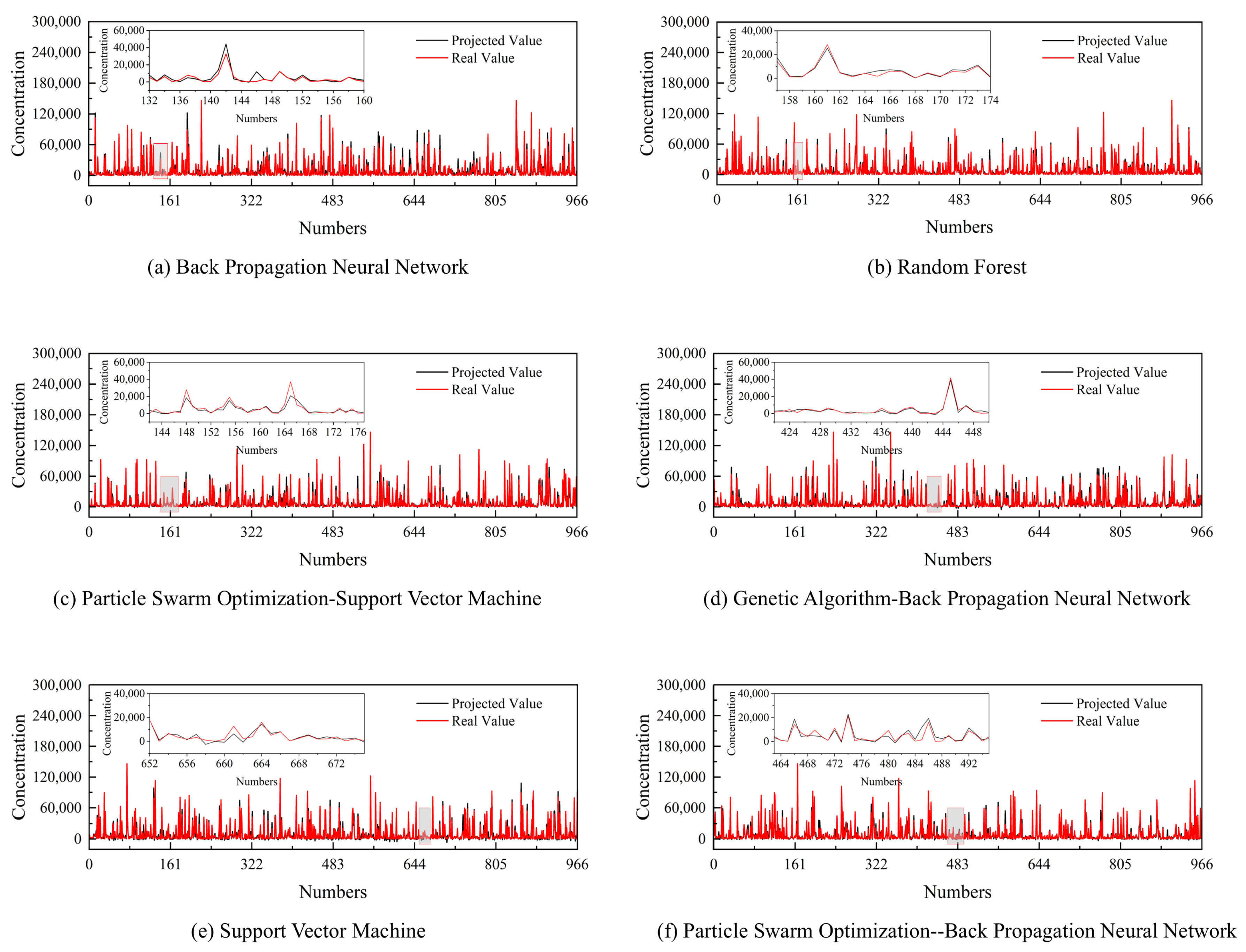
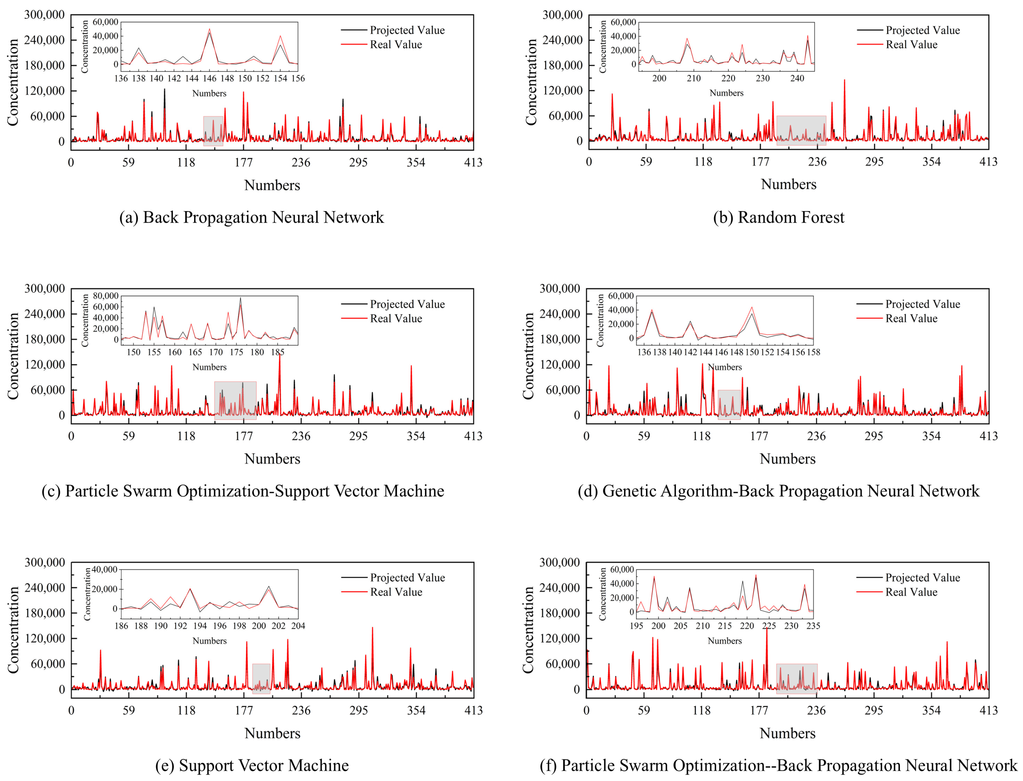
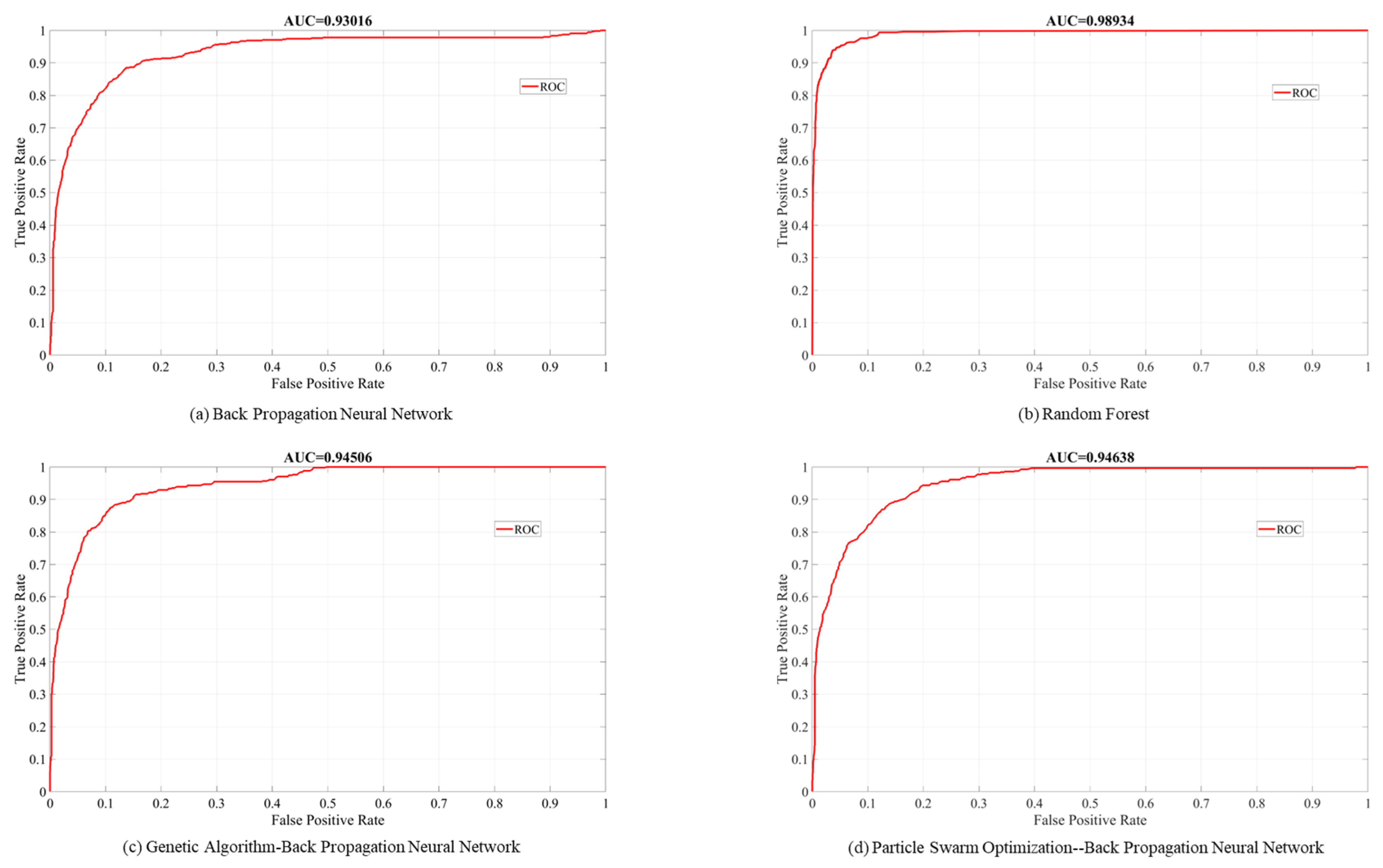
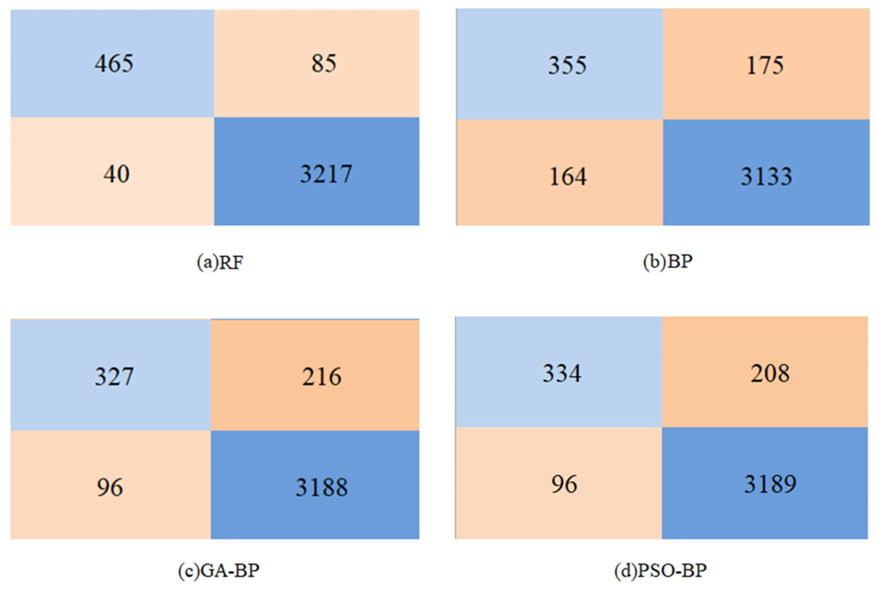
4.2. Comparison of Machine Learning Model Performance

Currently, there is a lack of literature exploring the application of machine learning techniques for predicting concentrations of exported oil and gas using multi-parameter inputs, and no information exists regarding the optimal machine learning model to achieve superior accuracy and precision in addressing this prediction problem. The present study employs six algorithms, namely, a BP Neural Network, a Support Vector Machine, and Random Forest, to forecast the concentration of exported oil and gas. Through the above steps, it is finally determined that the data volume of the regression prediction model is 1379, all of which are collected from the field of the oil depot. The input features are 8, and the output is the export oil and gas concentration (mg m⁻³). All the prediction models adopt normalized pretreatment methods.

Table 4. Performance index parameters (MAE—mean absolute error; R²—Coefficient of Determination).

	Training Set R2	Test Set R2	The Average R2 After Cross-Validation	Training Set MAE	Test Set MAE	The Average MAE After Cross-Validation
BP	0.8897	0.8422	0.8758	3677.3227	3935.7610	3421.2937
SVM	0.8906	0.8724	0.8621	2999.3626	3079.9374	3381.9632
RF	0.9438	0.9314	0.9081	1814.3089	2533.9995	2602.8601
PSO-BP	0.9010	0.8964	0.8880	3430.7646	3627.3885	3252.7312
PSO-SVM	0.9165	0.9011	0.8816	2498.2642	2969.0997	3232.0596
GA-BP	0.9101	0.9036	0.8894	3074.3935	3075.3705	3314.7126

shows the performance indicators of each algorithm and the performance indicators after cross-verification. The K-fold cross-verification method is adopted in this paper, where k is set to 5. Comparison graphs between the true and predicted values of the test set and training set for the six models with superior performance among those mentioned above are depicted in Figure 6 and Figure 7. It can be observed that while there is a small discrepancy between the predicted and true values in regions of low exported oil and gas concentration, a significant difference exists in regions of high oil and gas concentration. Nevertheless, these curves effectively capture the overall trend of changes in oil and gas concentration.

Among these six models, the machine learning method with the best performance index is the Random Forest algorithm, which achieves a goodness of fit (R²) of 0.9314 on the test set. The mean absolute error (MAE) is the smallest among the various methods in the model with a magnitude of mg m⁻³. To visually compare the size of the MAE, it needs to be normalized, resulting in the normalized mean absolute error (NMAE). The specific formula for calculating the NMAE is as follows.

$$NMAE={\displaystyle \frac{{{\displaystyle \sum }}_{i=1}^n\left|{\widehat{y}}_l-y_i\right|}{{{\displaystyle \sum }}_{i=1}^n{y}_i}}$$

(17)

where $\widehat{y_i}$ is the predicted value in the model, and $y_i$ is the true value entered in the model.

The NMAE calculated is shown in

Table 5. NMAE for each algorithmic model (NMAE—normalized mean absolute error).

	Training Set NMAE	Test Set NMAE
BP	0.29296	0.32769
SVM	0.29113	0.3414
RF	0.17776	0.26125
PSO-BP	0.31286	0.32712
PSO-SVM	0.28781	0.34514
GA-BP	0.30623	0.3394

. The NMAE achieved by the Random Forest algorithm for model prediction can reach 0.26, indicating a mean accuracy of 0.74, surpassing that of other prediction models. Furthermore, the Random Forest model demonstrates superior accuracy in predicting pollutant concentrations compared to other multi-parameter inputs [34]. The accuracy of this model surpasses that of other prediction models, and the Random Forest model exhibits superior accuracy in comparison to other multi-parameter input pollutant concentration predictions.

In the study above, it was found that the regression model incurs a large prediction error when the oil and gas concentration is high. The regression model is prone to overfitting the training set during the training process, particularly when there are fewer high-concentration data points. This implies that the model may excessively rely on these sparse data points when learning about the high-concentration region, resulting in a larger prediction error in that area and making it difficult to generalize to other similar high-concentration situations. The results provided by the regression model are typically exact values, which may impose excessive accuracy requirements in certain practical applications. However, fluctuations in oil and gas concentrations are inherently associated with certain uncertainties, and the exact predicted value may not always be necessary, especially in high-concentration cases where substantial fluctuations and uncertainties may occur. Classification models, by transforming the concentration prediction task into a discrete classification problem, not only simplify the prediction task but also effectively address the challenges faced by regression models at high concentrations.

When using classification methods for prediction, it is essential to limit the number of process parameters considered in the actual control process as some parameters are interrelated and their connections are difficult to observe directly from the data. Consequently, it is necessary to experiment with various combinations of predictions when employing machine learning methods for classification. Since the operation of the condensing unit results in minimal changes in the temperature of the adsorption tank, the dataset used for classification prediction was extracted after being divided according to the pressure of the adsorption tank without further screening based on the temperature of the adsorption tank. The final dataset comprised 12,627 entries. The same five machine learning algorithms were utilized for classification prediction. Figure 8 and

Table 6. Performance metrics for four classification models.

Arithmetic	Accuracy	Precision	Recall	FPR
BP	91.6%	68.4%	67.0%	5.0%
RF	97.2%	92.1%	84.5%	1.2%
GA-BP	91.8%	77.3%	60.2%	3.0%
PSO-BP	92.1%	77.7%	61.6%	2.9%

present the performance metrics of four of the more effective machine learning algorithms. The indicators in Table 6 were derived from the confusion matrix in Figure 9. Following a correlation analysis and excluding parameters with weak correlations, the final inlet oil and gas concentration, inlet oil and gas temperature, outlet temperature of the refrigeration unit, and compressor outlet temperature were identified as the most suitable combinations of input variables.

As shown in Table 6, the Random Forest algorithm achieves the highest accuracy of 97.2%, significantly outperforming the BP Neural Network (91.6%), GA-BP Neural Network (91.8%), and PSO-BP Neural Network (92.1%). This indicates that Random Forest has a substantial advantage in the overall correct prediction rate. The precision rate indicates the proportion of samples that the model predicts to belong to the positive category and are indeed in that category. In contrast, the recall rate assesses the model’s capability to correctly identify samples within the positive category. In terms of precision rate, Random Forest leads with 92.1%, while the BP Neural Network exhibits the poorest performance, with a precision rate of only 68.4%. In terms of recall rate, Random Forest (84.5%) also outperforms the other algorithms, whereas the BP Neural Network has a recall rate of 67%, indicating its limited ability to capture positive class samples. The false-positive rate reflects the proportion of negative class samples misclassified as positive, with lower values being preferable. Random Forest has the lowest false-positive rate of 1.2%, demonstrating its strongest ability to discriminate between negative classes. In contrast, the BP Neural Network has a higher false-positive rate of 5.0%, indicating that it is less capable of distinguishing negative class samples. AUC (Area Under Curve) reflects the overall classification performance of the model and is an important indicator of the model’s capability. The AUC value for Random Forest is 0.98934, which is significantly higher than that of the BP Neural Network (0.93016), GA-BP Neural Network (0.94506) and PSO-BP Neural Network (0.94638). This further demonstrates the superiority of Random Forest in classification performance.

In summary, the Random Forest model is the optimal choice for this study due to its excellent classification performance and robustness. Additionally, the incorporation of Genetic Algorithms (GAs) and Particle Swarm Optimization (PSO) based on the backpropagation (BP) Neural Network can enhance classification performance to some extent, with PSO-BP outperforming GA-BP, though it still does not match the overall performance of the Random Forest. This is mainly due to the fact that Random Forest enhances the generalization ability of the model by integrating the ensemble learning mechanism of multi-decision trees, and alleviates the local optimal problem caused by the hyperparameter sensitivity of BP Neural Network. Additionally, it addresses the high computational cost of SVM when dealing with high-dimensional data. Moreover, RF has fewer hyperparameters to tune; it primarily requires adjustments to the number of decision trees and their maximum depth. In contrast, BP Neural Networks necessitate fine-tuning several parameters such as learning rate, number of hidden layer neurons, and training iterations, which increases the risk of overfitting. Furthermore, RF demonstrates superior performance while consuming less computational time and resources compared to some optimization algorithms that require greater computational effort.

5. Conclusions

In this study, the RF algorithm was employed to predict the outlet oil and gas concentration in oil and gas recovery devices, and its performance was compared with that of the BP Neural Network, SVM, PSO-BP, PSO-SVM, and GA-BP. The results demonstrated that RF outperforms other models in terms of prediction accuracy, model stability, and computational efficiency. The R2 of the Random Forest regression model can reach more than 0.9, and the error can be controlled within 18%. In the classification model, the Random Forest model also shows excellent performance, which can increase the accuracy and accuracy of the model to more than 90%. Moreover, RF effectively handles nonlinear relationships and complex feature interactions, automatically evaluates feature importance, and selects the most relevant features. Although optimization-based models like PSO-BP, PSO-SVM, and GA-BP help refine parameter selection, they involve significant computational overhead and are still susceptible to local minima. Furthermore, RF can be utilized to optimize process parameters and operational workflows, helping oil depots reduce energy consumption in recovery devices without significantly affecting oil and gas recovery efficiency, thereby achieving cost reduction and efficiency improvement.

References

1. Ahsan, M.; Tian, L.; Du, R.; Alhussan, A.A.; El-Kenawy, E.-S.M. Optimizing Environmental Impact: MCDM-Based Approaches for Petrochemical Industry Emission Cuts. IEEE Access 2024, 12, 35309–35324. [Google Scholar] [CrossRef]
2. Zhang, Y.; Yu, Q.; Yuan, Y.; Tang, X.; Zhao, S.; Yi, H. Adsorption Behavior of Mo-MEL Zeolites for Reducing VOCs from Cooking Oil Fumes. Sep. Purif. Technol. 2023, 322, 124059. [Google Scholar] [CrossRef]
3. Al-Muhtaseb, S.A. Effects of Adsorbent Characteristics on Adiabatic Vacuum Swing Adsorption Processes for Solvent Vapor Recovery. Chem. Eng. Technol. 2006, 29, 1323–1332. [Google Scholar] [CrossRef]
4. Shie, J.-L.; Lu, C.-Y.; Chang, C.-Y.; Chiu, C.-Y.; Lee, D.-J.; Liu, S.-P.; Chang, C.-T. Recovery of Gasoline Vapor by a Combined Process of Two-Stage Dehumidification and Condensation. J. Chin. Inst. Chem. Eng. 2003, 34, 605–616. [Google Scholar] [CrossRef]
5. Shi, L.; Huang, W. Sensitivity Analysis and Optimization for Gasoline Vapor Condensation Recovery. Process Saf. Environ. Protect. 2014, 92, 807–814. [Google Scholar] [CrossRef]
6. Nitsche, V.; Ohlrogge, K.; Stürken, K. Separation of Organic Vapors by Means of Membranes. Chem. Eng. Technol. 1998, 21, 925–935. [Google Scholar] [CrossRef]
7. Roizard, D.; Lapicque, F.; Favre, E.; Roizard, C. Potentials of Pervaporation to Assist VOCs’ Recovery by Liquid Absorption. Chem. Eng. Sci. 2009, 64, 1927–1935. [Google Scholar] [CrossRef]
8. Chiang, C.-Y.; Liu, Y.-Y.; Chen, Y.-S.; Liu, H.-S. Absorption of Hydrophobic Volatile Organic Compounds by a Rotating Packed Bed. Ind. Eng. Chem. Res. 2012, 51, 9441–9445. [Google Scholar] [CrossRef]
9. Wang, Y.; Gan, Y.; Huang, J. Hyper-Cross-Linked Phenolic Hydroxyl Polymers with Hierarchical Porosity and Their Efficient Adsorption Performance. Ind. Eng. Chem. Res. 2020, 59, 11275–11283. [Google Scholar] [CrossRef]
10. Fu, L.; Zuo, J.; Liao, K.; Shao, M.; Si, W.; Zhang, H.; Gu, F.; Huang, W.; Li, B.; Shao, Y. Preparation of Adsorption Resin and Itas Application in VOCs Adsorption. J. Polym. Res. 2023, 30, 167. [Google Scholar] [CrossRef]
11. Feng, X.; Sourirajan, S.; Tezel, F.H.; Matsuura, T.; Farnand, B.A. Separation of Volatile Organic Compound/Nitrogen Mixtures by Polymeric Membranes. Ind. Eng. Chem. Res. 1993, 32, 533–539. [Google Scholar] [CrossRef]
12. Wang, H.; Lu, Q.; Zhang, Z.; Lin, J.; Wu, Q. Study on Separation of CO2 Condensation from Natural Gas Based on Cellular Automaton Method. Energy Sources Part A Recovery Util. Environ. Eff. 2024, 46, 3663–3683. [Google Scholar] [CrossRef]
13. Sikiru, S.; Soleimani, H.; Shafie, A.; Olayemi, R.I.; Hassan, Y.M. Prediction of Electromagnetic Properties Using Artificial Neural Networks for Oil Recovery Factors. Colloid J. 2023, 85, 151–165. [Google Scholar] [CrossRef]
14. Ghanem, A.; Gouda, M.F.; Alharthy, R.D.; Desouky, S.M. Predicting the Compressibility Factor of Natural Gas by Using Statistical Modeling and Neural Network. Energies 2022, 15, 1807. [Google Scholar] [CrossRef]
15. Wang, F.; Tang, X.; Deng, C.; Li, J. Application of BP Neural Network to Prediction of Recovery Effect of Air-Foam Flooding in Heavy Oil. Pet. Sci. Technol. 2022, 40, 1914–1924. [Google Scholar] [CrossRef]
16. Liu, X.; Wang, Q.; Wen, Y.; Li, L.; Zhang, X.; Wang, Y. Comparison of Ethane Recovery Processes for Lean Gas Based on a Coupled Model. J. Clean. Prod. 2024, 434, 139726. [Google Scholar] [CrossRef]
17. Orru, P.F.; Zoccheddu, A.; Sassu, L.; Mattia, C.; Cozza, R.; Arena, S. Machine Learning Approach Using MLP and SVM Algorithms for the Fault Prediction of a Centrifugal Pump in the Oil and Gas Industry. Sustainability 2020, 12, 4776. [Google Scholar] [CrossRef]
18. Yue, M.; Dai, Q.; Liao, H.; Liu, Y.; Fan, L.; Song, T. Prediction of ORF for Optimized CO2 Flooding in Fractured Tight Oil Reservoirs via Machine Learning. Energies 2024, 17, 1303. [Google Scholar] [CrossRef]
19. Hong, B.-Y.; Liu, S.-N.; Li, X.-P.; Fan, D.; Ji, S.-P.; Chen, S.-H.; Li, C.-C.; Gong, J. A Liquid Loading Prediction Method of Gas Pipeline Based on Machine Learning. Pet. Sci. 2022, 19, 3004–3015. [Google Scholar] [CrossRef]
20. Cen, X.; Chen, Z.; Chen, H.; Ding, C.; Ding, B.; Li, F.; Lou, F.; Zhu, Z.; Zhang, H.; Hong, B. User Repurchase Behavior Prediction for Integrated Energy Supply Stations Based on the User Profiling Method. Energy 2024, 286, 129625. [Google Scholar] [CrossRef]
21. R Azmi, P.A.; Yusoff, M.; Mohd Sallehud-din, M.T. A Review of Predictive Analytics Models in the Oil and Gas Industries. Sensors 2024, 24, 4013. [Google Scholar] [CrossRef] [PubMed]
22. Zhai, S.; Geng, S.; Li, C.; Gong, Y.; Jing, M.; Li, Y. Prediction of Gas Production Potential Based on Machine Learning in Shale Gas Field: A Case Study. Energy Sources Part A Recovery Util. Environ. Eff. 2022, 44, 6581–6601. [Google Scholar] [CrossRef]
23. GB 20950-2007; Emission Standard of Air Pollutant for Bulk Gasoline Terminals. National Standards of People’s Republic of China: Beijing, China, 2007.
24. Cui, K.; Jing, X. Research on Prediction Model of Geotechnical Parameters Based on BP Neural Network. Neural Comput. Appl. 2019, 31, 8205–8215. [Google Scholar] [CrossRef]
25. Wang, C.-D.; Xi, W.-D.; Huang, L.; Zheng, Y.-Y.; Hu, Z.-Y.; Lai, J.-H. A BP Neural Network Based Recommender Framework With Attention Mechanism. IEEE Trans. Knowl. Data Eng. 2022, 34, 3029–3043. [Google Scholar] [CrossRef]
26. Zhang, L.; Wang, F.; Sun, T.; Xu, B. A Constrained Optimization Method Based on BP Neural Network. Neural Comput. Appl. 2018, 29, 413–421. [Google Scholar] [CrossRef]
27. Wang, L.-L.; Ngan, H.Y.T.; Yung, N.H.C. Automatic Incident Classification for Large-Scale Traffic Data by Adaptive Boosting SVM. Inf. Sci. 2018, 467, 59–73. [Google Scholar] [CrossRef]
28. Aisyah, S.; Simaremare, A.A.; Adytia, D.; Aditya, I.A.; Alamsyah, A. Exploratory Weather Data Analysis for Electricity Load Forecasting Using SVM and GRNN, Case Study in Bali, Indonesia. Energies 2022, 15, 3566. [Google Scholar] [CrossRef]
29. Jakkula, V. Tutorial on Support Vector Machine (Svm); School of EECS, Washington State University: Pullman, WA, USA, 2006; Volume 37, p. 3. [Google Scholar]
30. Khan, A.U.; Salman, S.; Muhammad, K.; Habib, M. Modelling Coal Dust Explosibility of Khyber Pakhtunkhwa Coal Using Random Forest Algorithm. Energies 2022, 15, 3169. [Google Scholar] [CrossRef]
31. Zhang, X.; Shen, H.; Huang, T.; Wu, Y.; Guo, B.; Liu, Z.; Luo, H.; Tang, J.; Zhou, H.; Wang, L.; et al. Improved Random Forest Algorithms for Increasing the Accuracy of Forest Aboveground Biomass Estimation Using Sentinel-2 Imagery. Ecol. Indic. 2024, 159, 111752. [Google Scholar] [CrossRef]
32. Tian, K.; Kang, Z.; Kang, Z. A Productivity Prediction Method of Fracture-Vuggy Reservoirs Based on the PSO-BP Neural Network. Energies 2024, 17, 3482. [Google Scholar] [CrossRef]
33. Xu, C.; Li, L.; Li, J.; Wen, C. Surface Defects Detection and Identification of Lithium Battery Pole Piece Based on Multi-Feature Fusion and PSO-SVM. IEEE Access 2021, 9, 85232–85239. [Google Scholar] [CrossRef]
34. Dong, Q.; Fu, X. Prediction of Thermal Conductivity of Litz Winding by Least Square Method and GA-BP Neural Network Based on Numerical Simulations. Energies 2023, 16, 7295. [Google Scholar] [CrossRef]
35. Wang, M.; Xiong, C.; Shang, Z. Predictive Evaluation of Dynamic Responses and Frequencies of Bridge Using Optimized VMD and Genetic Algorithm-Back Propagation Approach. J. Civil. Struct. Health Monit. 2024, 15, 173–190. [Google Scholar] [CrossRef]
Figure 1. Process flow of the on-site oil and gas recovery device.
Energies 18 01078 g001
Figure 2. Pressure–temperature variation in the adsorption tank.
Energies 18 01078 g002
Figure 3. Schematic diagram illustrating the principle of the BP Neural Network [26].
Energies 18 01078 g003
Figure 4. Schematic diagram of the principle of a Support Vector Machine [29].
Energies 18 01078 g004
Figure 5. Pearson’s correlation coefficient heatmap.
Energies 18 01078 g005
Figure 6. Comparison of true and predicted values for test set samples.
Energies 18 01078 g006
Figure 7. Comparison of true and predicted values for training set samples.
Energies 18 01078 g007
Figure 8. ROC curve graphs for the test set (ROC—Receiver Operating Characteristic).
Energies 18 01078 g008
Figure 9. Confusion matrix for the test set.
Energies 18 01078 g009