Abstract
To maximize photovoltaic (PV) production, it is necessary to estimate the amount of solar radiation that is available on Earth’s surface, as it can occasionally vary. This study aimed to systematize the parametric forecast (PF) of solar energy over time, adopting the validation of estimates by machine learning models (MLMs), with highly complex analyses as inclusion criteria and studies not validated in the short or long term as exclusion criteria. A total of 145 scholarly sources were examined, with a value of 0.17 for bias risk. Four components were analyzed: atmospheric, temporal, geographic, and spatial components. These quantify dispersed, absorbed, and reflected solar energy, causing energy to fluctuate when it arrives at the surface of a PV plant. The results revealed strong trends towards the adoption of artificial neural network (ANN), random forest (RF), and simple linear regression (SLR) models for a sample taken from the Nipepe station in Niassa, validated by a PF model with errors of 0.10, 0.11, and 0.15. The included studies’ statistically measured parameters showed high trends of dependence on the variability in transmittances. The synthesis of the results, hence, improved the accuracy of the estimations produced by MLMs, making the model applicable to any reality, with a very low margin of error for the calculated energy. Most studies adopted large time intervals of atmospheric parameters. Applying interpolation models can help extrapolate short scales, as their inference and treatment still require a high investment cost. Due to the need to access the forecasted energy over land, this study was funded by CS–OGET.
1. Introduction
Numerous mechanisms that govern life on Earth are primarily driven by solar energy emitted on to the surface of the planet [1,2]. The best way to ensure that life continues as long as possible is to make the best use of this resource and turn it into a non-polluting technology of natural environmental cycles in order to create an endless supply of non-polluting energy [3], also known as renewable or green energy, that is sustainable and has low levels of pollution and energy consumption [4]. The rate of rural electrification is still very low, with approximately 80% of communities lacking access to electricity [5]. This lack is prevalent in many sub-Saharan African communities, particularly the Nigerian region, with Mozambique ranking sixth, with about 20 million people lacking access to electricity [6], many of whom live in rural and suburban areas [7]. The Sustainable Development Goals (SDGs), however, aim to minimize polluting gas emissions by 2050 and mandate electrification by the end of 2030 [5,8,9]. Fossil fuels contribute to global warming by their continued widespread use in many parts of the world today; thus, other energy sources are employed, such as nuclear power plants [10,11], which endanger human health and the environment, and hydroelectric power plants [12], which by themselves cause ecological harm and droughts [4,13]. The SDG aim of lowering net emissions by 2050 [12] is inspired by serious environmental issues [14]. Due to environmental concerns, increased energy needs, fluctuating fuel prices [15], rising costs, and the possibility of fossil fuel depletion, renewable and environmentally friendly green technologies have become more popular [14,16]. In order to make solar energy plants more competitive in the energy market [17] and decrease dependence on fossil fuels [18] for social and economic growth, solar energy forecasting is essential [19,20]. In light of the SDGs for global electrification, PV solar energy is becoming more and more popular as a low-cost, clean, efficient, and sustainable technology [6,15,21] that can be purchased anywhere around the globe [3]. One of the biggest challenges of the modern age is optimizing its operation [22,23]; understanding the many local solar input factors that are taken into account when sizing and installing PV power plants would be the best course of action to enhance these projects’ efficiency [3,15,16,17,18,19,20,21,22,23,24]. An estimated 80% of installed projects globally [25,26] exhibit various anomalies, ranging from solar optimization to appropriate device selection in the sizing model [27,28] and even analyzing energy variability across the regions of interest [2].
In order to achieve grid balance, recent studies have employed MLMs and methodologies to optimize and estimate solar energy utilizing samples of solar, wind, and tidal energy on multiple distinct time scales [29,30]. One study found that their ANN predicted 24 h global horizontal irradiation (GHI) well; on bright days, the correlation coefficient was between 98 and 99%, while on overcast days, it was between 94 and 96% [31,32,33]. In order to estimate GHI and the clear-sky index , researchers used hybrid models to forecast GHI in an island context, and the results showed potential for solar projections [34]. After analyzing aerosol optical thickness (AOT) over irradiance estimated using a normal aerosol scenario, it was concluded that, on average, +9 or approximated the world mean irradiance values very well, where the errors in direct normal and diffuse horizontal irradiance (DNI and DHI) balanced each other [35,36]. In addition to projecting solar energy and electrical load, it was observed that adjusting wind speed and irradiance from numerical weather prediction presented difficulties [37,38]. Precise energy forecasting from geographically dispersed solar generation resources was defined as crucial to enhance the penetration of solar generation resources into the electrical grid [39]. The researchers based their short-term solar forecasting solely on the measurements of GHI, coming to the conclusion that alternative models, while configurable, require further observations of several atmospheric parameters [40]. MLMs for daily solar energy forecasting using numerical climate models provide a large number of features that can deteriorate learning algorithms’ ability to generalize [41]. Forecasting power generation from renewable energy sources (RESs) like solar panels and wind turbines is becoming crucial for the power grid to run smoothly and continuously. It also aids in making the most use of RESs [42]. Significant sensitivity to variation in the forecast horizon and significance with regard to location selection were indicated by an analysis of the forecast horizon’s sensitivity to solar irradiance and ambient temperature [43]. One study examined the quantification of solar energy fluctuation variability at high frequencies using short-scale measurements and came to the conclusion that the correlation between high fluctuation variability rapidly diminishes at shorter intervals [6]. DNI prediction using multivariate regression (MVR) and MLMs was forecasted, and it was concluded that the lifetime of solar plants was increased when the size of the power plant was known [31,44]. GHI variability was predicted in another study, and the findings of the model tree technique could be used in real time to generate forecasts of solar variability, which can help utilities manage the power grid [45]. They used a gradient-boosted regression tree (GBRT) model, which was demonstrated to be competitive in terms of mean squared error (MSE) across all prediction horizons, to predict solar power at several locations [42,46]. Regression analysis was considered to simulate GHI for any point on Earth [4,47,48]. The models produced by regression analysis outperform existing models in solar irradiance forecast [49].
In areas around a GHI measuring station, where the precise GHI data are unknown even for the future, the primary goal of this research is to forecast solar energy using a parametric model applied to MLM. The same proven MLM parametrically forecasts the GHI sample’s future behavior and its behavior in the regions around it, providing the real variability of partial solar energy and quantifying solar energy availability on a short-scale measurement [2,50,51].
In light of the ePPI review platform’s summaries of 145 bibliographic sources that were accessed between 25 November and 30 November 2023, data from publicly available sources were gathered from Web of Science/of Knowledge, Science Direct, IEEE Xplore, Research for Life, and SCOPUS. These sources also covered knowledge of solar energy behavior in some hard-to-reach locations, like desert regions, paradisiacal high seas, wildlife reserves, and forests, among others, that may still be challenging to master. With this information, the primary issue with power may be resolved as it would enable modeling of the solar energy that is accessible in these locations and be used for a variety of local uses in addition to being injected into the grid [14,52]. Within this framework, the present research primarily focuses on many estimating requirements for solar energy estimates:
- ○
- They base their short-term solar projections solely on GHI measurements and conclude that more observations of different atmospheric factors are needed for other models, but they are configurable [40,53,54];
- ○
- They studied the quantification of the variability in solar energy fluctuations at high frequencies through short-scale measurements, concluding that the correlation between high fluctuation variability decreases at shorter intervals [4,55,56,57];
- ○
- Spatial estimation of sub-second, second, minute, sub-hourly, annual GHI using a combination of special approach, geostatistical interpolation methods, and Regression Kriging (RK) interpolation from in situ imagery to satellite data [21,39,58,59].
Considering that a portion of the population lacks energy and that the study region has restricted access to both comparable research and infrastructure, as well as recommendations for the design of energy usage projects [5,6], in response to the query, what factors go into the accurate forecast of solar energy availability using MLM? The daily GHI population was defined, and the participants were the years of measurements of the GHI sample from the station in the Province of Niassa in Nipepe. The comparisons that are made between the GHI predictions using different MLMs for parametrically forecasting the GHI, and the study of meta-analyses of spatial and temporal variability in solar energy availability and the outcome that the solar energy forecasted obtained, the sample of GHI data collected was validated, through the ePPI reviewer platform that shows some considerations of the objectives of the analysis with the comparison with the STATA Software statistical package platform, version 18.0. The current study’s methodologies seek to both boost forecast accuracy and correct the past forecasting systems’ lack of diversity.
The parametric forecast models were used for theoretical derivation and verification. Regression analysis was also used to compare the model’s estimation accuracy. Ultimately, we identified the best parameters to consider in a parametric forecast. The techniques used in this study introduce a more effective validation process by reducing performance error through the use of new meteorological correction parameters. This leads to improved performance in terms of recommending effective tools for the forecast GHI in station-less locations, as well as for a better evaluation of electricity consumption patterns and the choice of a more precise method to estimate future energy demand. The study of the parametric forecast solar energy and its variability using various MLMs is complemented by this research on solar energy variability.
2. Methods
2.1. Method Used
This systematic scope analysis review adopted to manage all collected data was associated with the bibliometrics method in reference management, a review that supports the evaluation and interpretation of thematic areas, and we used a protocol that included the following: research questions and hypothesis, search process, inclusion, and exclusion criteria, data selection, search methodology, and extraction process and data synthesis (available at https://github.com/Muco-1990/Protocole_Parametric_For_Var.git (accessed on 12 November 2024).
2.2. Inclusion and Exclusion Criteria
The inclusion of the reasoning with logic and the intricacy of the analysis justifies the sample access. According to the inclusion criteria, the articles had to meet the parametric validation of atmospheric components, address solar energy forecasting using MLM, use validation using solar energy samples measured in situ or by remote sensing in short- and long-term measurement scales, and use complexity of reasoning in their titles, abstracts, keywords, and article composition. Studies with samples not in short-scale measurement (0.01 s to 24 h) or long term (up to 1 year) were eliminated based on the exclusion criteria, as were studies that did not validate their findings using MLM.
2.3. Sources of Information and Materials
Utilizing the ePPI reviewer platform available at https://eppi.ioe.ac.uk/eppireviewer-web/home (accessed on 5 November 2023), the bibliographic sources were accessed and included a range of roughly 145 sources of the most recent analysis. The following search terms were used: “forecasting solar energy, solar energy trends, parametric forecast, solar energy availability”. Research for Life available at https://www.sciencedirect.com/ (accessed on 6 November 2023), SCOPUS available at https://www.scopus.com/home.uri (accessed on 16 November 2023), and Web of Science/Knowledge available at https://www.webofscience.com/wos/alldb/basic-search, (accessed on 10 December 2023) were among the other access sources from which data were obtained between 1 November and 25 December 2023. The literature linking articles was carefully selected and examined over 23 years. After that, the chosen terms were input into a reference management system, which generated a file format for keyword analysis in a research information system. Networks of scientific keywords were created using the VOS viewer program available at https://app.vosviewer.com/ (accessed on 12 November 2024) and linked by a co-occurrence link, which is a relationship between two phrases. The quantity and strength of the co-occurrence, which illustrate the viewpoints and patterns of keywords like forecast, spatiotemporal, variability, parametric, GHI, and assessment, were determined by the word’s size.
2.4. Selection and Data Gathering
After examination, the articles were pulled into bibliometric databases so that any potential duplicates could be automatically removed. The online collection was accessed through the flowchart, which made it possible to identify recurrent references and modified versions that shared the same analytical focus. The researchers’ physical examination made it possible to thoroughly examine and remove repeats. However, about six items that were duplicates were found in the databases that were checked during the process. https://github.com/Muco-1990/parametric_for_systematic_review.git (accessed on 22 November 2024) contains their consultation. Data, such as authors, title, method, model, doi, abstract, country, climate, error, and keywords, were already taken out of the identified papers. On average, there were about 145 items that were connected to the literature. The data extraction form that the researchers employed was specifically linked to the seven study topics. As illustrated in Figure 1, which shows the delimitation of articles for the systematic review using the Prisma approach, a peer review validation was carried out to verify the identification of the responses. If there were any differences, agreements were reached for the selection of the responses to achieve full data verification.

Figure 1.
Diagram of Prisma flow for solar energy forecasting [60].
Additionally, Figure 1 provides a declaration of the research’s adherence to the PRISMA 2020 guidelines [60]. It was filed on the Shiny platform (https://prisma.shinyapps.io/checklist/) on 13 November 2024, with ID: 12566. As previously mentioned in the preceding paragraphs, Figure 1 illustrates the overall adherence to all writing standards, beginning with identification, screening, retrieval, eligibility, and inclusion. This adds up to the systematic review of the literature on parametric solar energy forecasting with a focus on MLM and validation for in situ measurement stations.
2.5. Informational Data Items
To forecast solar energy variability, the search and extraction of the data sample mainly involved an optimal optimization of the solar energy forecast models. The expected results include a forecast of direct, diffuse, and global solar irradiance; spatial behavior of solar energy; the relationship of solar energy with other renewable energy generating resources; estimation of measurement errors; and variability of atmospheric parameters over time, aerosol concentration, water vapor, ozone layer, uniformly mixed gases, among others. Using solar energy collected in situ or from remote sensing, the studies give various metrics of measurement intervals ranging from 0.0001 s to 24 h, primarily in time intervals of about 1 h, from the set of over 145 sources that were investigated. When these findings from other research for measuring and assessing solar energy fluctuation are included, the current study’s conclusion becomes more evident. Similar to the outcome, the extracted sources likewise specify correlation measurements between local and distant measurement stations, apply MLM to draw a haphazard conclusion, and, most importantly, estimate the origin of several climatic parameters while focusing just on local reasons. This study, however, is anticipated to produce a result in which the generalized reason for each region of operation is already measured by the aggregated parameters alone.
2.6. Measures of Bias and Effect
A variety of models were employed. The majority of studies take into account models like simple linear regression and Kriging regression, but others also tend to use the RF, ANN, and their variants, which estimate lower risks of bias when assessed through peer review with key stakeholders. The measured data deviation for each sample source was caused by the keywords’ relative distance from the previously specified keywords. A summary of the data margin and its categories was provided by the synthesis. Showing an average of 145 sources overall, the majority of which are not estimated, the estimated models’ measurement errors range from 10 to 15 W/m2. Considering that the absorbed energy would rise to 1362 W/m2, a value near the theoretical solar constant, the results are consistent and demonstrate a massification of energy through the correction of parameters of climatic, atmospheric, and other origins, in an average of 900 W/m2 of the measured energy. The sample’s meticulous presentation established a correlational analysis with the production over the years, as well as the cumulative analysis.
2.7. Bias Evaluation
The sample is included in the list of data that have an ambiguity but are applicable; typically, this is in the group of applications of the MLM that illustrate a greater margin of estimation of solar energy. The bibliometric method showed a series of sample references with their references for missing data and presenting a lot of deviation outside the desired characteristic. However, for higher-quality data extraction, physical analysis and exploratory analysis were continued in addition to the bibliometric method. The instrument error plus computational processing of 0.001, the observation error of 0.00001, and the relative error calculated from a 99% confidence level were all taken into consideration when determining the sample error for statistical analysis. Given that the range level is 5 in every scenario, interpolative models were used to address the model’s automatic interpretation errors. Additionally, the RF model yielded a fair interpretation, with an error of about 0.01.
2.8. Search Methodology
This study employed ePPI review techniques for keyword analysis and linkages to 23-year-old literature. By building scientific keyword networks with co-occurrence relationships, a research information system was developed utilizing VOS reader software version 1.6.20. The magnitude of the words affected the co-occurrence strength. Data from many sources, such as Web of Science/Knowledge, Science Direct, IEEE Xplore, Research for Life, and SCOPUS, were compiled utilizing the bibliometrics approach, which employed scoping analysis and systematic review techniques. To predict solar energy trends and availability, this study examined 145 bibliographic sources. Based on the fewest instances of a particular term, 679 relevant keywords with the highest overall link strength were found.
Due to the limited post-processing output over 23 years, the systematic review was examined utilizing a large number of keywords and bibliographic sources as of 2024. The bibliometrics approach in the program’s reference management was combined with the research development method in the information system to improve data management and the ePPI reviewer 6 platform’s search and analysis of bibliographic sources. Data samples, GHI measurements, cloud speed, and solar energy estimates were examples of cross-cutting components.
This study focuses on the variables that affect how solar energy availability is estimated by an MLM. It analyzes the daily GHI and solar radiation behavior and compares parametric models, , and MLM results for stakeholder Niassa. Since the GHI inferred by a pyranometer is complete on Earth’s surface, the analysis sample, collected as part of the FUNAE effort between 2020 and 2021, was selected to validate the range of complete observations from dawn to dark. With a positive correlation between 2001 and 2024, high relative output in 2018 and 2022, and roughly 679 interconnected keywords, the bibliographic source sample was registered in ePPI Reviewer 6 version 6.15 on January 10, under ID 52365. This study used STATA software version 18.0 available at https://www.stata.com/new-in-stata/ (accessed from 1 to 26 November 2023), to examine data and discovered similar meta-analyses, with a focus on parametric energy efficiency calculations. The validated GHI sample must be used to analyze new findings. The research issue, according to the systematic review, is “Parameterization Forecast solar energy over time by applying Machine Learning Techniques,” underscoring its scope and limitations.
2.9. Data Synthesis
A strategy of extracting materials that met the inclusion criteria aided in addressing the research difficulties through database search and analysis. The qualitative method of applied content analysis, which occasionally drew from bibliometric sources, was founded on an exploratory and interpretative component. It developed and extracted objective judgments from the whole reading of the body bibliometric memory for each model. The first phase involved organizing the data in the study region. Next, key data was extracted using the inclusion criteria’s PRISMA 2020 rules and the research questions. The data that was extracted was triangulated, examined, and validated by peer review. The responses were merged with an existing classification to allow for possible analysis and interpretations. Statistical analysis and VOS version 1.6.20, were used to identify interesting intersections of terms, keywords, co-term networks, categories, and subcategories. The data on the quantity of sources and their variation across all years, both geographically and temporally distributed, are analyzed using causal inference approaches. The solar energy sample used to validate the parametric model of solar energy forecasting using MLM is described in the paragraph that follows.
2.10. Solar Energy Data Collection and Processing
The analysis sample was gathered from the National Energy Fund (FUNAE) [61] and consisted of a sample of GHI data obtained during the solar radiation measuring campaign conducted by FUNAE in 2020 and 2021 at the Nipepe station (reference FUNAE–MZ06–Nipepe) in the northern region of Mozambique. To measure the radiation component of GHI and DHI, pyranometer sensors were used, as shown in Figure 2, in conjunction with a system in which a pyrheliometer was inserted to determine the DNI component directly.

Figure 2.
Pyranometer used to measure GHI during the campaign (FUNAE).
The ideal calibration parameters for the pyrheliometer (Eppley–type) that was utilized to gather the data were set to: calibration factor 295–2800 nm, spectral range with 1-min response, linearity ±0.5%, ±1%. A portion of the information was gathered at the National Institute of Meteorology (INAM) [62] and at Eduardo Mondlane University (UEM). This included sample data on solar radiation measured in situ with an automatic Davis station and a pyranometer, as illustrated in Figure 3, as well as measurements of temperature, wind, moisture, greenhouse gases, aerosols, and greenhouse gases.
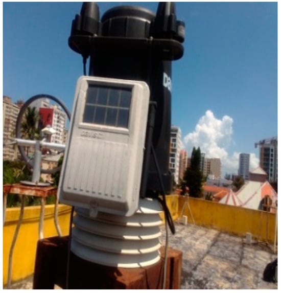
Figure 3.
Davis automatic station (INAM).
The meteorological and atmospheric variables were taken from the Aerosol Robotic Network (AERONET) [63] database, which included a sample of aerosol optical thickness (AOT) measured by a sun photometer. These variables were then verified in the same database, producing calibrated results with the help of developed algorithms that, by themselves, already provided some quantities that were relevant to our analysis of the values collected in 1 min measurement intervals as well as daily, hourly, monthly, and annual average intervals. Values of aerosol optical mass, precipitation, and multiple reflectance by gases were precisely collected at the Niassa stations, represented in Table 1, which is available for the years 2020 and 2021.

Table 1.
Coordinates of the measurement stations.
Samples were taken at short-scale intervals of around four minutes, one minute, one hour, one day, and monthly averages from measurements taken between 19 June 2019 and 31 December 2023. They were measured using data from AERONET, which is obtained through the sun photometer, which gathers light absorbed by aerosols in the upper and lower atmosphere at different wavelengths of identification, AERONET instrument number 1187. The data have multiple levels, including Level 1 and 1.5, but these have been updated and more precisely measured, along with the removal of additional anomalies discovered in Level 2.0 treatment measurements for all stations of the data collected.
Regular seasonal maintenance, including data transfer, battery replacement, cleaning, and realignment, was performed on each device during the measurements.
The sample was collected at the Nissa station, which is situated between the parallels 10°27′ and 26°52′ south latitude and between the meridians 30°12′ and 40°51′ east longitude. The cleaning and orientation periods were recorded during this process, except for data selection periods, such as periods of interference and turbulence. The local topographic section of the measuring station and its latitude and longitude characteristics are displayed in Figure 4.

Figure 4.
Data sample collection site Niassa Province in Northern Mozambique.
As seen in Figure 5, in the first step, a sample of bibliographical reference data was collected in the database and registered, after it generated a link of keywords related to the parametric models applied to MLM. This led us to collect a sample of the data, which were next subjected to quality control, spurious value removal, and processing by programs created especially for computing radiation with a 10 min time interval, joined to the AERONET atmospherically, meteorological, spatiotemporal predictor variables. That helped to consider a better choice of different atmospheric parameters considered in the presented parametric model. In the third level, these data were applied to validate the model and registered in the ePPI version 6.15 and STATA version 18.0, which showed a link of possible meta-analysis, as depicted in the last level of Figure 5.
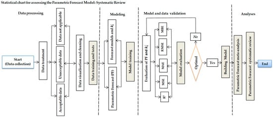
Figure 5.
Statistical design of parametric model building.
2.11. Evaluation and Effects of the Fuel Sources Currently in Use
According to available data, between 2010 and 2023 [47], the number of individuals not covered by the electrical grid increased by 83% to 91%, from 733 million para 1.2 billion [5,64]. In the interim, to massify renewable actions by more than 30% (net-zero emissions by 2050), dominated by fossil fuels [42,65], electrification efforts are still necessary to achieve the ambitious global electrification outlook by 2030 and to overcome the slowdown of 0.8 to 0.5 percentage points from 2010 to 2018 and 2018 to 2020 [66,67]. In 2020, the percentage of people without access to electricity worldwide who live in rural regions increased by 1% [5,36] annually, with the largest increase occurring in sub-Saharan Africa [24]. Approximately 80% of this population lives in these areas. Approximately 76% of the world’s population lives in the 20 countries with the largest access deficits [26,68]. Mozambique ranks sixth, with roughly 20 million of citizens affected [4,5]. These factors also include interannual oscillations, which are strong variations in cloud cover and rainfall, El Niño and La Niña episodes [3,69], determinants of intermittent temporal fluctuations in solar energy [15,70], etc., which contribute to the existence of life on Earth [64,71].
To fulfill the predicted worldwide demand of 800 GW by 2050 [5,7] and reduce air pollution, the Mozambique Electricity (EDM) declared an expected PV capacity of 50 MW by the end of 2023, with expected expansion in the future [5,25]. The performance of PV systems and the size of battery storage are the primary areas of the 5 MW total PV capacity (stand-alone and grid-connected PV systems) in Mozambique’s Mid–North region that are impacted by solar energy fluctuation.
From seconds and meters [72] to days and thousandths of kilometers [6,66], variability in solar radiation increments can span a wide range of spatiotemporal scales [34,70,71,72,73]. This variability affects generation, load balancing, and power quality maintenance, such as voltage and frequency stability [6].
Generally speaking, primary sources contribute roughly 78% of the energy that keeps fossil fuels strong (4% comes from nuclear power and 74% from fossil fuels). It is significant that these fossil fuels have detrimental effects on the ecosystem. On the other hand, as Figure 6a,b demonstrates, the Sun provides roughly 22% (1% direct solar energy, 21% indirect solar energy, and 0.2% geo, ocean, and environment) to the production of clean, safe, and environmentally healthy energy [5,6,71].
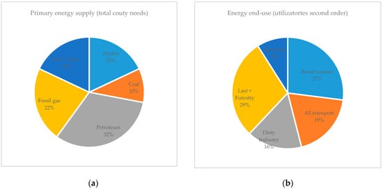
Figure 6.
Illustration of local energy scenario. (a) Primary energy and its usage rate; (b) Applicability and destination of energy waste as well as beneficiary.
Generally speaking, a variety of instruments can be used to measure solar radiation depending on how well they work. It is significant to note that the radiometer is the fundamental tool used to measure solar radiation [3,26].
2.12. Synthesis Methods
The intervention and assessment of solar energy using atmospheric parameters and other factors determined the eligibility of the studies retrieved for each synthesis; nevertheless, they must meet the established eligibility requirements. Other factors employed in the decision-making process included operationalization using MLM, decreased error estimates, and sample validation using solar energy measured primarily in situ. The cumulative model creates a summative tabulation of the data, the correlative model extracts the data to correlate the studies among themselves, and the inferential model extracts the causal analysis of the tabulated data to tabulate or visually display the results of individual studies and syntheses; all were employed as auxiliary analyses in the data preparation process.
2.13. Research and Data Validation
This study introduces an algorithmic model that offers a structured methodology for analyzing, extrapolating, and forecasting solar radiation at the nuclear station and its associated neighboring stations. In contrast to other algorithms that rely on assumptions based on limited solar irradiance data, this approach is applicable on a global scale. Prior research has indicated that predicted values often deviate significantly from actual measurements, resulting in substantial errors. Here, the application of standard RF and ANN models algorithms in the parametric model resulted in a notably reduced internal error, compared to the reported mean absolute error (MAE) of 10.2 and 7.12 W/m2 [50,74]. Although literature models incorporate local meteorological parameters, such as climate, weather, seasons, humidity, latitude, longitude, and altitude, for various applications, they demonstrate commendable performance in testing and predicting energy efficiency.
2.14. Extraction and Correction of Raw Data
A maximum at noon is a characteristic of the data processing. The scripts created especially for computing radiation with a time interval of 10 (ten) minutes were applied to this data sample after it had first undergone quality control and spurious value removal. Regular seasonal maintenance, including data transfer, battery replacement, cleaning, and realignment, was performed on each device during the measurements. Except for data selection events such as periods of interference and turbulence, cleaning and orientation phases were documented during this procedure.
Next, the data process involved treating the GHI sample beforehand to reduce potential losses from errors, also known as uncertainty or margin of error (error), and to acquire data from direct GHI measurements. After that, the information was taken out of the Logger database and made available for confirmation. Forecasting solar energy throughout the hours of sunshine, or from sunrise to sunset, is crucial from the perspective of solar energy consumption. Nevertheless, some days had insufficient data for a variety of reasons, including bird demands and obstructions to measurements, pyranometer shadowing, and a decrease in convection energy for devices that rely on local information.
However, interpolation techniques were used, among other things, to fill in these gaps in the data and make repairs. Data were taken from the original, in situ measurements. Next, models were used to forecast data on solar energy, and the corresponding measurement errors were found. Most of the models under consideration are machine learning models built using cutting-edge artificial intelligence techniques.
2.15. Parametric Estimation of Total Solar Energy
Upon reaching the Earth’s horizontal surface, solar radiation is subject to various factors such as atmospheric and environmental typology [23,44]. These are categorized based on factors, like atmospheric activity, atmospheric properties (such as the ozone layer and greenhouse gases), surface characteristics (such as albedo and vegetation), astronomical and geographic factors (such as altitude and angle of incidence), climatic effects, and climatic events. The troposphere stretches from 8 to 15 km, the stratosphere stretches from 15 km to 50 km [5,34], the mesosphere stretches from 50 km to 85 km, the thermosphere stretches from 85 km to 600 km, and the exosphere stretches from 600 km to 10,000 km; these are the various layers that make up Earth’s atmosphere [7,9,23]. These layers are determined by temperature gradients and other factors [3,6,53].
Various researchers propose different methodologies for predicting and estimating solar energy. However, a common issue arises as each author presents their estimates regarding the percentage of solar energy received and the factors contributing to its attenuation. For instance, the estimative model for solar energy, positing that solar insolation is influenced by wavelength, is represented by the equation [24,69]. This model acknowledges the solar constant while noting that approximately 30% of sunlight is diminished as it traverses the Earth’s atmosphere before reaching the surface. This reduction is attributed to various effects, including Rayleigh scattering by the atmosphere, particularly at shorter wavelengths, which follows a dependency of , as well as scattering by aerosols and dust particles and absorption by atmospheric gases, such as oxygen, ozone, water vapor, and carbon dioxide [3,6]. Specifically, 7% of sunlight is scattered to the Earth (the diffuse component), 3% is scattered into space, and 18% is absorbed by ozone at altitudes of 20–40 km, upper dust layers at 15–25 km, air molecules from 0 to 30 km [7,9,10,11,12,13,14,15,16,17,18,19], water vapor from 0 to 60 km, and lower dust from 0 to 90 km, with an additional 3% scattered into space [6,24].
Another estimate on numerical models begins by assuming that direct radiation alone can predict 100% of solar energy [11,16]. However, this also takes into account the existence of atmospheric attenuation and considers that, in addition to the direct radiation measured on Earth’s surface, diffuse radiation, which results from diffuse radiation caused by scattering and absorption by aerosols, gases, and water vapor, must be added [3]. This total proves that there is global energy on Earth’s surface.
Other literature provides that only 50% of the 100% of solar radiation that is emitted in short and long waves reaches the Earth’s surface as direct and/or diffuse radiation [3,15]; the remaining 16% is absorbed by particles of , and other greenhouse gases; 4% is absorbed by clouds [35]; and 30% is fully reflected as solar shortwave, with 6% of the radiation being backscattered by air molecules, 20% reflected in clouds, and 4% reflected on the surface of the Earth [75].
The light can be impacted by the following processes: (1) atmospheric scattering by air, water, and dust molecules; (2) atmospheric absorption by , and . These phenomena are detailed in Iqbal [3,45]. Most radiation travels through an air mass (AM) to reach the Earth’s surface throughout the day when the sky is clear. The path that solar radiation takes from its incidence in the atmosphere to the Earth’s surface is known as the air mass , where is the angular distance between the solar beam and the vertical that touches the zenith of the incidence site [15].
The radiation is analyzed as being at its minimum in the winter and at its greatest in the summer, so the declination of the radiation at the research site was estimated over the daily course for days of year, given by Equation (1) [7,15].
whose position relative to the sun for horizontal surfaces is given by Equation (2) [16,75],
A typical zenithal angle equal to 90 degrees, resulting in a solar angle , given by Equation (3) as [3,6],
The length of the day is determined according to the rule, which is equal to 2, given by Equation (4) [15].
The difference in minutes between solar time and standard time is given by Equation (5) [15,75].
where is the Standard Meridian for the local time zone, and is the longitude of the location in question, measured in degrees ,
The eccentricity correction factor of the Earth’s orbit in Equation (6) is [3,24],
The equation of time presents variables along the year, presenting positive evaluation in the last days of the end year, in its optimal development, and having the shape as in Figure 7.
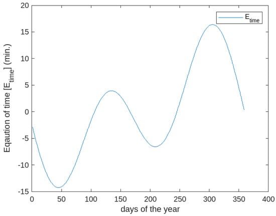
Figure 7.
Equation of time time-series days of year.
The zenith angle is given by Equation (7) [3,24]
The relative optical air mass is calculated by Equation (8) [3]
The relative optical mass of the air, considering the pressure in mbars, is determined by Equation (9) as [69,76],
Reduced precipitable water w, with w′ the precipitable water, is given by Equation (10) [3,77]
The transmittances for the direct insolation of individual atmospheric constituents are compared in detail, assuming the multiplicative total transmittance due to the transmittances for direct irradiance due to absorption by ozone () [3,27], the transmittances for direct irradiance due to absorption by water vapor (), the transmittance for direct irradiance due to attenuation by aerosols () [10,31], the transmittances for direct irradiance due to absorption by uniformly mixed gases () [3], and the transmittances for direct irradiance due to Rayleigh scattering effect of air molecules () [10,19], so the total transmittance is a multiplicative of all transmittances, as given in Equation (11) [32],
The multiplicative transmittance for the Nipepe-2 station is displayed in Figure 8, with an average of roughly 0.5281 in 2021 compared to roughly 0.5267 in 2020.
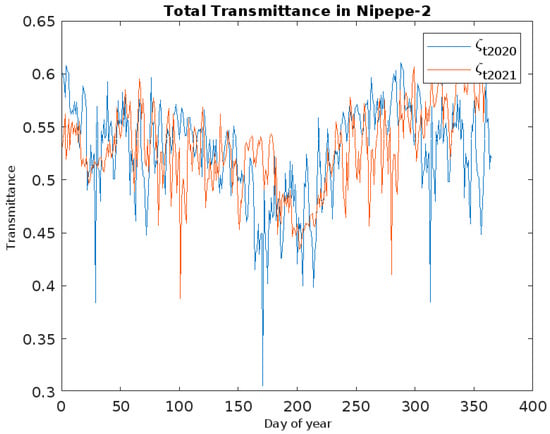
Figure 8.
Transmittance for direct irradiance due to total at Nipepe-2 in Niassa, in the years 2020 and 2021.
Comparing equations where each absorptance is considered differently is informative. The transmittance via Rayleigh scattering is driven by Equation (12) [15,78],
The ozone transmittance, influenced by the constant deposition of the emitted gases is given by Equation (13) as follows [3]:
in which defines . Figure 9 illustrates that the numerical values obtained are within approximately 0.071 of each other, even though the test conducted at the same measurement station reveals that there are different concentrations of the ozone layer for different years, with the concentrations rising to 0.9232 in 2020 due to greenhouse gas emissions over the region of consideration.
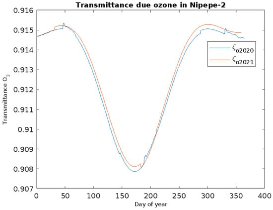
Figure 9.
Ozone transmittance as a function of day of the year, at Nipepe-2 in Niassa, in the years 2020 and 2021.
As can be seen in the previous diagram, the biggest variation in this one is , which was established for AERONET average measurement. These variations depend on the zenith angle and the amount of ozone present. Because ozone has a very high transmittance, it has very little effect on the total transmittance. The following yields the transmittance by direct irradiance caused by uniformly mixed gas absorption, given by Equation (14) [3,10,79]:
Figure 10 illustrates the reduced attenuation of the transmittance for direct irradiance resulting from absorption by uniformly mixed gases (), with an average of roughly 0.9873 for 2020 and 2021.
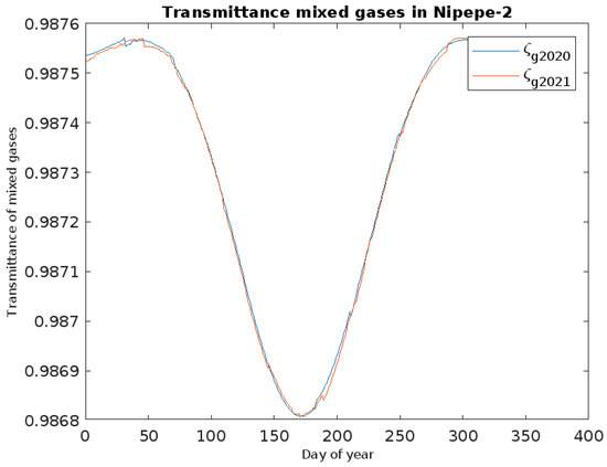
Figure 10.
Transmittance for direct irradiance due to absorption by uniformly mixed gases as a function of the day of the year, in Nipepe-2 in Niassa, in the years 2020 and 2021.
In the summer months, there is an increased excitation of these gases due to the effects of temperature, which leads to the formation of systems that exhibit enhanced absorption and transmission [6,75]. Conversely, during the dry and cold seasons, these gases significantly attenuate solar energy, thereby limiting the direct impact of this radiation on the Earth’s surface [25]. This results in a period of instability in solar energy utilization, necessitating careful management of the excess energy generated and careful consideration in the final solar balance calculations to appropriately size the solar system based on the measured energy. Additionally, we examined mathematical models to estimate solar energy availability, assess local grid penetration rates, and identify the variability in cloud cover and atmospheric aerosol concentrations [80,81], as well as the indirect influence of atmospheric gases, to a lesser extent [82]. The transmittance of water vapor is given by Equation (15) as [3,44,56],
is defined here. With an average transmittance of 0.9059 in 2020 and growing to 0.9073 in 2021, the variances between the transmittance in those two years are about the same. As Figure 11 indicates, the variations with the zenith angle over the course of the year are related to the amount of water vapor, with cm serving as an example.
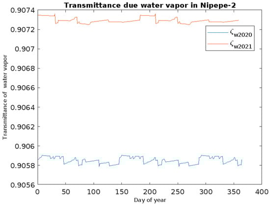
Figure 11.
Direct irradiance as a function of precipitable water, at Nipepe-2 in Niassa, in the years 2020 and 2021.
An analysis employing precipitable water with a proportion of 2 cm and O3 with a proportion of 0.85 cm revealed that the GHI spectrum yields higher values [3,83]. No matter how visible it is, the difference is always somewhat less than 25. Considering that there is only a 0.089 difference between the two solar constants, this is an intriguing result.
Provide a different load on populations of particles known as aerosols released into the atmosphere to obtain an expression for the aerosol transmittance of this model. This expression is based on the spectral attenuation at the two wavelengths that the meteorological network typically uses, 400 and 659 nm, which are the wavelengths where ozone molecular absorption is least, as given by Equation (16) [3],
In this case, . Different databases and country services routinely measure the thickness of aerosols at these wavelengths. One can disregard a measurement at a wavelength if it is uncertain. An equation for ta in terms of the Angstrom turbidity parameters and , or visibility, will be helpful in places where turbidity or visibility is reported. According to an analysis, the concentration in Nipepe-2 to 0.8547 in 2021 from roughly 0.8538 in 2020 are shown in Figure 12.
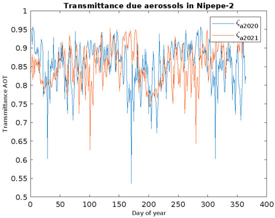
Figure 12.
Transmittance for direct irradiance due to attenuation by aerosols , in Nipepe-2 in Niassa, in the years 2020 and 2021.
For irradiance, transmittance, and absorptance, the direct irradiance, also known as direct normal irradiance that reaches the earth’s surface, is provided and is further generalized by Equation (17) as [32,56].
When the spectral range is taken into account for solar radiation (0.3–3 nm), the factor 0.9751 is added as a result in Equation (18) [24,56],
Higher certainty is obtained in the estimation of solar irradiance (at various time scales) through the use of geographic coordinates like latitude and longitude, as well as meteorological parameters, like cloud cover , sunshine duration , clearness index , pressure , air temperature , relative humidity , wind speed , wind direction , etc.
We report results for a clean atmosphere accounting for aerosol attenuation. The spectrally integrated results for a clean atmosphere with equal to 4 cm and equal to 0.89 cm, are very good at , illustrating a mean of 657.4009 with a deviation of 104.0978 in 2020 and 657.80865 with a deviation of 104.0978 in 2021. Figure 13 shows the direct normal irradiances obtained constituting a spectrally integrated approach.
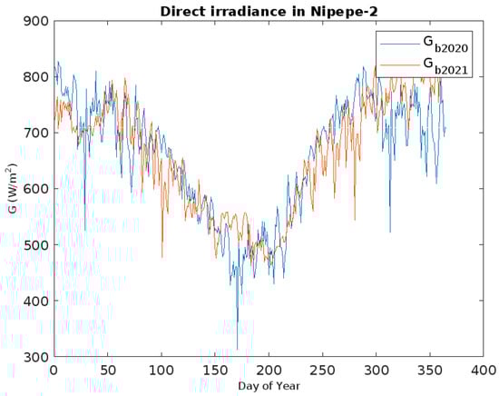
Figure 13.
Direct normal irradiance of a clean atmosphere obtained from various models, at Nipepe-2 in Niassa, in the years 2020 and 2021.
The impact of turbidity was measured at of visibility, with equal to 3 cm and equal to 0.89 cm. Nearly equivalent findings are obtained at zenith angles less than , particularly at greater zenith angles. Nevertheless, for outcomes in broadband computations, the first few millimeters of precipitable water in the atmosphere attenuate.
In Figure 13, whether the atmosphere is empty or laden with of water vapor, the findings will yield an essentially equal degree of error, given an average ozone standard of 0.89 and a visibility of for of precipitable water. A modification in the visibility parameter can demonstrate that this statement essentially stays the same. This finding helps create a more straightforward parameterization equation with a constant [15,35].
The method used to determine the irradiance on a horizontal surface is predicated on the findings from two areas of study. Following its initial passage through the atmosphere, Rayleigh scatters diffuse irradiance, which is determined by Equation (19) as [3],
Diffuse radiation (), which results from a variety of events, interacts with stuff in the atmosphere as depicted in Figure 14.
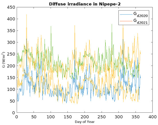
Figure 14.
Diffuse irradiance, at Nipepe-2 in Niassa, in the years 2020 and 2021.
As can be seen, the ozone layer, aerosol deposition, uniformly mixed gases, and geometric variables all influenced in 2021 (orange line), which was near to the theoretical in 2021 (green line) with average maximums of and . On average, however, was higher in 2021 than it was in 2020 (blue line), when it averaged a maximum of .
Here, we take to represent the direct radiation transmittance due to the aerosol absorptance, because of the diffusion, given by Equation (20) [3,24,81],
The diffuse irradiance dispersed by aerosols following their initial passage through the atmosphere is determined by, and should be assumed to be, 0.9 unless a more precise value for w0 is provided, by Equation (21) as [3,15],
where was previously defined by Equation (22) [75,84,85]
Until more precise data on aerosols become available, this model suggests using a constant value of 0.84 for . The diffuse irradiance measured an average of 112.8236 in 2020, increased by a percentage to an average of 112.5279 in 2021, and deviated to 38.5645 in 2021, as depicted in Figure 15.
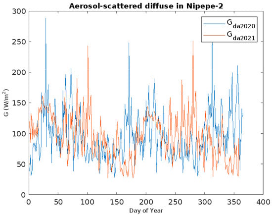
Figure 15.
Aerosol–scattered diffuse in Nipepe-2 in Niassa, in the years 2020 and 2021.
As , the quantity of aerosols in the atmosphere, grows, so does the atmospheric albedo. With an increase in , the atmospheric albedo likewise rises [75]. More small particles are represented by an increase in α, because small particles scatter more radiation than large particles [85]. The spectrogram for multi-reflected diffuse radiation looks like this [3,14]. The GHI on a horizontal surface is compared with its behavior in Figure 16.
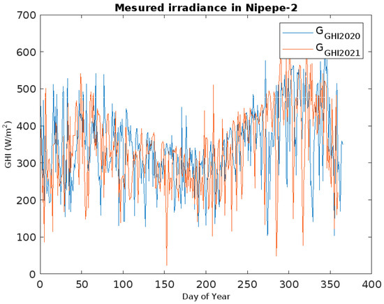
Figure 16.
Measured irradiance, at Nipepe-2 in Niassa, in the years 2020 and 2021.
It yields numbers that are less 2020 than in 2021, mostly because, in the model, the diffuse components differ from one another. Once more, the atmospheric turbidity factors determine how different they are, as shown in Figure 17 [35,86].
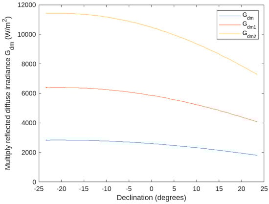
Figure 17.
Variation of the cloudless sky albedo as a function of turbidity parameters, in Nipepe-2 in Niassa, in the years 2020 and 2021.
The difference between lower and higher values is determined by the characteristics of air turbidity. Before contrasting the diffuse irradiance produced in the two years, the atmosphere’s albedo, or , with α and β, as illustrated in Figure 17, rises with β as predicted. This is a representation of the quantity of aerosols in the atmosphere [6,87,88]. As the value of α grows, so does the atmospheric albedo; since small particles scatter more radiation than large particles, a rise in α indicates a greater concentration of small particles [3,15,56].
The atmospheric albedo has been proposed to have the formula given in Equation (23), to achieve the multiple reflected irradiance [3,75,77]:
The difference between the two formulations for albedo is not based on the air mass expression [3,10,19]. The scattering of light between the Earth and the atmosphere is due to many reflections. This is one way to write the diffuse irradiance [25]: . The global irradiance (rightmost diffuse) on the horizontal surface can be given by Equation (24) as [69,89]
The global irradiation on a horizontal surface is compared in Figure 18.
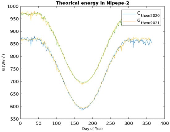
Figure 18.
Theoretical energy, in Nipepe-2 in Niassa, in the years 2020 and 2021.
The deposition of particles that block the path of solar radiation spreads and diffuses a lot during the hot and rainy season (September to February), as shown in Figure 18. This is primarily caused by the geometric orientation of the earth at this point of analysis (Nipepe), which exposes it to the maximum incidence of solar radiation. This results in maximum transmittances and a consequently greater incidence of solar energy, with a maximum theoretical portion, predicted to be in the range of in 2020 and in 2021.
However, there is a minimum incidence of solar radiation during the cold and dry season (March to August), which is marked by the earth’s diametrically opposite geometric orientation in the region of analysis. This helps to maintain the stationarity of particles deposited in the atmosphere by a variety of effects and causes, forming even more consistent layers that contribute significantly to maximum attenuation, absorption, and reflectance. There is also a minimum transmittance of solar energy to the earth’s surface, resulting in a minimum incidence of solar energy in the range of in 2021 and in 2020.
To put it briefly, the theoretical global energy forecasted for 2021 (orange line) is nearly equal to the theoretical energy for 2021 (green line), which is even higher than that of 2020 with an average difference of in both years, with the least amount occurring in the cold and dry season and the most during the hot and rainy season. The diffuse components of the two years differ, which is the main cause of the decreased numbers, and the atmospheric turbidity factors determine how different these years are. To rectify the parametric association, MLMs were employed, which may be explained as follows:
Training data for Simple Linear Regression (SLR) with continuous variables and GHI were obtained for values , and provided by Equation (25) [74,90,91].
With identical independence, the errors have the following values: , . The regression line represents the estimate , which is given as for the expected value of the condition [92].
The random forest (RF) model uses three neighborhoods with a search scope of , with a spatial dataset GHI and a neighborhood of station . The neighborhood-averaged is represented by , while the weighted average counterpart is represented by based on inverse distance weighting [2,35,93].
The equation measures the relative inverse distance weights between stations, with being an exponent parameter that amplifies the relevance of closer neighbors while reducing the weights of more distant ones. A larger exponent indicates greater influence of nearby points on predicted values.
We employed the Regression Kriging (RK) model, which combines the expected residuals from Kriging with the projected regression trends as provided by [49,90,93],
If the number of auxiliary variables is p, the estimated regression coefficients , a constant term is , the residual is , and the trend (climatic and geographic variables) is represented by . With each neuron having an input range of , multiplied by the weights , and gathered in neuron j specified by Equation (28), the Artificial Neural Network (ANN) model was utilized [33,94].
This includes the bias, denoted as . For a value , to which an activation function is applied, an expression for this function is [33]. As opposed to a basic linear or exponential regression, whose output has a normal distribution produced by a linear relationship, the Support Vector Machine model (SVM) [95] was employed. It can be regular, binomial, or Poisson.
considering as a function to map a nonlinear input of coefficients using a kernel function, and are the weight vectors. The ARIMA model is an analytical statistical model that uses time-series data to understand and forecast future trends, as given by Equation (30) [74,96]
The variables are independent variables that are identical to them in the sample to the normal distribution with mean zero; L is the lag operator; αi is the parameter of the autoregressive section of the module; is parameters of the moving average in terms of error. Regression classification is conducted using a model called Gradient-Boosting Machines (GBMs). It builds a forecasting model by combining decision trees. When we take into account regression values, the forecast for the initial prediction shown in Equation (31) becomes [90,97],
A potent nonparametric Bayesian regression method that offers flexibility in modeling intricate relationships in data is Gaussian Process Regression (GPR). Pretend that there is a Gaussian process before functions, given in Equation (32) as [32,43,97],
where , the covariance (or kernel), the likelihood of detecting u given GHI for GPR, and the function of the day are denoted by m(GHI), , and so on [32,96].
Networks with Long Short-Term Memory (LSTM): This is a collection of recurrent neural networks (RNNs), which are intended to learn from a sequence of data and provide predictions. is the forget gate (gates determine what position is given the cell state to have); dt (hidden state) is the output of the LSTM unit and is used for prediction and contains information about constant time weight, and (cell state) represents the memory of the trajectory [96].
The input gate determines whether part of the data is reduced. The association between a time series and its lag values is measured by the autocorrelation function (ACF). The autocorrelation function at a lag of for a time series , and [32,96,97],
where stands for variance and covariance. The autocorrelation between and that is not explained by the lags between them is represented by PACF, which stands for [97,98].
3. Results of Forecasting Solar Energy and Analysis of Systematic Bibliographic Sources
3.1. Parametric Forecasting of Solar Energy
3.1.1. Spectral Distribution Histograms for Days
As seen in Figure 19, the anticipated data sample has a high frequency of values with high levels of solar irradiation in the order of 1241.85 W/m2.
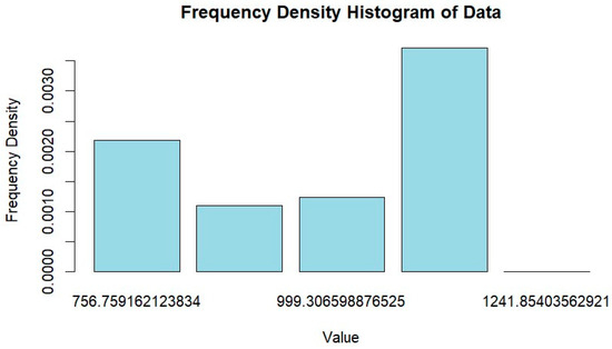
Figure 19.
Spectral distribution of GHI histograms of year days.
The analysis conducted over one day, as depicted in Figure 20, reveals a significant correlation between the values predicted by the parametric models, with correlation coefficients nearing 0.989. Conversely, the estimated radiation shows an even higher correlation, with values around 0.9999 when utilizing in situ measurements. Furthermore, Figure 20 also indicates that the radiation on the horizontal surface aligns closely with the theoretical spectrum, thereby enhancing the parametric estimation of solar energy. This observation demonstrates the presence of full Sun conditions with a high incidence of solar energy under clear-sky conditions or skies with minimal cloud cover.

Figure 20.
Qualitative analysis of performance and intensity of irradiance types.
3.1.2. Autocorrelation and Partial-Autocorrelation Function
The energy levels in each model are quantitatively represented using the autocorrelation function (ACF), which has an average order of 0.8956 as shown in Figure 21. Additionally, the parametric analysis is enhanced by the partial-autocorrelation function (PACF) for the years 2020 and 2021, which has an order of 0.9896. The parametric analysis reveals that the solar energy described by the ACF gradually declines, while the one described by the PACF cuts after a few delays, as illustrated in Figure 21, based on the MLM tested with reduced error. But for the other MLM models, including ARIMA, LSTM and others, solar energy has been steadily declining for both ACF and PACF analysis. This demonstrates the extent to which the models used as input in MLM models are adequate, significantly boosting the estimate’s accuracy.

Figure 21.
ACF and PACF correlation function, in Nipepe-2 in Niassa, in the years 2020 and 2021.
3.1.3. Comparison Between Forecasted, Measured, and Theoretical Solar Energy
The solar energy forecast at the Nipepe station for 2020 and 2021 is very similar, with a margin of 0.01%, and both are very close to the theoretical irradiation spectrum (Figure 22). This observation improves parameterization through MLM, which accepts a set of parameters as input that are corrected using the MLM characteristics.
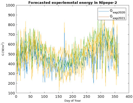
Figure 22.
Forecasted experimental energy, in Nipepe-2 in Niassa, in the years 2020 and 2021.
Considering all atmospheric factors that affect the solar radiation effect, the forecasted 2021 solar energy (orange line) is around the theoretical solar energy (green line). Additionally, the projected solar energy for 2020 (blue line) is around the same magnitude as the projected solar energy for 2021 (orange line). Yet, as expected based on the observation of standard theoretical radiation in Figure 18, the predicted experimental radiation follows the theoretical radiation spectrum, peaking in the months with the highest transmittance because of atmospheric parameters and falling in the months with the lowest transmittance.
Additionally, the forecasted energy in Figure 22, shows relatively little variation between 2020 (blue line) and 2021 (orange line), with 2021 showing a slightly higher quantitative incidence intensity. However, if it is greater in magnitude because it aggregates the energy absorbed by several parameters in its total estimate, compared to the solar energy measured on-site presented in Figure 15, this, in turn, is estimated to be less in 2020 than in 2021 and is mostly because, in the model, the diffuse components differ from one another. In the characteristics of solar energy incidence in the study location (Northern Mozambique), both forms of energy precisely track the development of theoretical irradiation. The behavior in 2020 and 2021 is determined by the previously mentioned spatiotemporal, climatic, and geographic elements of order, which obstruct solar radiation in its route. Figure 22 shows that energy levels are highest from September to March throughout the summer and lowest from April to August, with July serving as a climax.
3.2. Analysis of Systematic Bibliographic Data Sources
3.2.1. Every Technique for Forecasting Worldwide Horizontal Radiation
The process of forecasting GHI entails estimating the quantity of solar radiation that will arrive at a horizontal surface at a given place within a certain time frame [3]. Numerical weather prediction (NWP) models, satellite-based methods, hybrid approaches, machine learning techniques, and physical models (such as simplified radiation models and radiative transfer models) are some of the approaches and methods used for this purpose. Empirical models include regression analysis and artificial neural networks (ANNs) [99].
Solar radiation can be predicted using a variety of machine learning algorithms, such as support vector machines, random forests, and gradient-boosting machines, which are based on historical data and meteorological inputs.
The availability of input data, computational capacity, required forecast accuracy, and application requirements are some of the variables that influence the technique selection.
Additionally, validation datasets should be used to test the accuracy and dependability of the model’s performance because machine learning approaches can capture intricate correlations.
Artificial Neural Network (ANN) Model
These have interconnected nodes, referred to as neurons, arranged in layers, closely resembling the composition and operation of biological brain networks [100]. Feedforward neural networks, recurrent neural networks (RNNs), and convolutional neural networks (CNNs) are the three categories into which they can be separated. The fact that these are frequently used to forecast solar radiation makes them interesting. The model accurately predicted 24 h solar irradiation, and its quality was demonstrated by the correlation coefficient, which ranged from 94–96% for cloudy days to 98–99% for sunny days [32,101,102]. As shown in Table 2, decision tree and neural network models seem to be reasonable substitutes for the stepwise regression model in terms of comprehending energy consumption patterns and forecasting energy consumption levels, in addition to predicting electricity consumption [103,104]. These models’ ability to learn nonlinear correlations between input meteorological variables (such as temperature, humidity, and cloud cover) and GHI is one of their main features. This ability enables ANNs to be used to represent complex atmospheric processes [94,105].
Table 2.
Artificial neural networks (ANNs) for solar energy forecasting worldwide.
Support Vector Machine (SVM) Model
Both classification and regression tasks can be completed by this model at the same time. In a nonlinear feature space, it can be effectively used for GHI prediction by mapping meteorological inputs to GHI values [120,121]. Regression was used to estimate solar irradiance using all-sky image characteristics, and a mean absolute error of roughly 22% may be obtained when predicting 5 min solar irradiance [122]. It was demonstrated that predicting electricity consumption is a feasible substitute for analyzing energy consumption trends and estimating energy consumption levels [104]. One benefit of support vector machines (SVMs) is their consideration of an appropriate hyperplane for data point separation in a high-dimensional feature space [48,123]. This hyperplane is optimized to maximize the margin between classes, as further discussed in Table 3’s references [104,122].
Table 3.
Support vector machines (SVMs) for solar energy forecasting worldwide.
Random Forest (RF) Model
This involves creating several decision trees during the training process and calculating the average prediction made by each tree [93]. It was applied to phases of testing and development, where the mean absolute percentage error (MAPE) ranged from 3.8% to 13.8% [71]. The tool was employed to enhance the mapping of solar irradiance at high latitudes and produced a new dataset with higher accuracy and precision than the input datasets. The results included a bias of −1.5 W/m2 and 4.3 W/m2, a root mean square deviation (RMSD) of 17.9 W/m2 and 27.1 W/m2, a mean absolute deviation (MAD) of 11.9 W/m2 and 17.5 W/m2, and a bias of 0.01 W/m2 [2]. They can handle big datasets with high dimensionality, and they are resistant to overfitting [128,129,130]. As seen in Table 4, they may be utilized to predict GHI values by identifying patterns in meteorological data and forecasting GHI values based on input features.
Table 4.
Random forests for solar energy forecasting worldwide.
Gradient-Boosting Machine (GBM) Model
A collection of ensemble learning techniques is employed to construct models in a sequential manner, where each subsequent model addresses the errors of its predecessors [138,139]. The Pearson correlation coefficient was utilized to determine the most pertinent meteorological data for model training, revealing significant errors and demonstrating the study’s quality and reproducibility [14,20]. The researchers forecasted diffuse solar irradiance through machine learning and multivariate regression approaches. In the context of multivariate regression, the mean absolute error (MAE) for logistic regression, utilizing the aforementioned predictors, was recorded at less than 21.5 W/m2 and 30 W/m2 [140,141]. This method is particularly advantageous for effectively managing structured data and capturing intricate relationships. It has been successfully applied to global horizontal irradiance (GHI) prediction tasks, achieving high accuracy by progressively refining predictions based on the residuals from earlier models [140,141,142,143,144], as detailed in Table 5.
Table 5.
Gradient-boosting machines (GBMs) for solar energy forecasting worldwide.
Long Short-Term Memory (LSTM) Network Model
A specific kind of recurrent neural network (RNN) is used to represent sequential input and identify long-term relationships [144,145]. First, the structural effect accounts for the largest portion of the total contribution to consumption, reflecting the importance of solar energy growth [88,139,140,141,142]. The factorial decomposition and prediction of solar energy consumption were carried out, and the results show that the proposed approach combined with LSTM has better feasibility [145,146]. Its ability to learn patterns and trends from previous meteorological data, illustrated in Table 6, makes it advantageous for application in time-series forecasting, particularly GHI forecasting [142,146,147,148,149,150,151,152,153,154,155,156,157,158].
Table 6.
Long short-term memory (LSTM) networks for solar energy forecasting worldwide.
Gaussian Process Regression (GPR) Model
The link between the input and output variables is modeled as a multivariate Gaussian distribution using this nonparametric Bayesian technique. Investigations into the specific heat capacity of nanofluids for solar energy applications led to the conclusion that GPR performs better than RF and GRNN results [131]. As Table 7 illustrates, it has the benefit of being able to produce probabilistic GHI projections and quantify forecast uncertainty. It has been used for GHI forecasting assignments, especially when estimating uncertainty is important.
Table 7.
Gaussian process regression (GPR) for solar energy forecasting worldwide.
Autoregressive Integrated Moving Average (ARIMA) Model
As demonstrated in Table 8, they used the autoregressive integrated moving average (ARIMA) method to forecast solar energy consumption after breaking down the factorial. The findings indicate a larger share of total consumption, highlighting the significance of solar energy growth [32,88].
Table 8.
Autoregressive integrated moving average (ARIMA) for solar energy forecasting worldwide.
Simple Linear Regression (SLR) Model
However, several satellites provide these raw samples with an emphasis on estimated accuracy [2,162] compared to solar irradiation measured by traditional sensors that offer the real performance of solar energy on the Earth’s surface, used in the present research, with a margin of error of 0.3 to 0.5 [2,3,6]. An analysis and study of solar energy conditions that affect the region that is related to access to horizontal solar irradiation incident on that location were conducted. They used multivariable regression and machine learning to predict diffuse solar irradiation [2,3]. The mean absolute error (MAE) of logistic regression utilizing the aforementioned predictors was less than 21.5 W/m2 when the multivariable regression approach was applied, as shown in Table 9 [2,3,6].
Table 9.
Simple linear regression (SLR) for solar energy forecasting worldwide.
Regression Kriging (RK) Model
This machine learning model tackles regression in conjunction with correction variables [81]. With an equivalent rise in local network penetration rates, the MLM approaches marginally enhance the results. The worldwide horizontal irradiance at the sub-hourly level was estimated spatially using three geostatistical interpolation techniques, and Regression Table 10 indicates that 67% of the volunteer stations investigated present results within the margin of error (mean of ±2 standard deviations) according to Kriging interpolation from satellite photos [131]. Table 10 illustrates the benefits of obtaining results that are near to the estimate, among other things.
Table 10.
Regression Kriging (RK) for solar energy forecasting worldwide.
Hybrid Machine Learning Models
This consists of combining multiple machine learning models to increase estimation efficiency for comparisons and results [34,184,185,186]. According to [81], there was a comparable rise in local network penetration rates. Table 11 illustrates how applying machine learning techniques somewhat enhanced the performances reported by [34]. Its benefit is that it can provide more accurate projections based on the situation [29,44,69,186,187,188,189,190,191,192,193,194,195].
Table 11.
Hybrid machine learning models for solar energy forecasting worldwide.
Where HDKR is the Hay, Davies, Klucher, and Reindl model; NWM is the numerical weather model; NWP is the numerical weather prediction; the Multiscale Hybrid Forecasting Model (MHFM) USA, UK, MFDFA, tree-based ensemble machine learning models, and the United States of America are terms used to describe the United States and the United Kingdom, respectively. Random Forest (RF); Extra trees (ET) and decision trees (DT) the support vector regression (SVR); Angstrom–Prescott linear regression, or A-PLR for short; forward-looking neural networks, or F-FNNs; multiple linear regression, or MLR for short; CSI: conventional spatial interpolation; PCR: principal component regression; linear regression (LR), Gaussian process regression (GPR), generalized regression neural network (GRNN), multiple regression (MR), geostatistical interpolation (GSID), deterministic and HelioSat2 (GBRT), ARIMA stands for autoregressive integrated moving average in neural networks; S-SLA stands for single-site linear autoregressive; GM(1, 1) for grey prediction models; NGBM(1, 1) for the model and the grey Verhulst model.
By identifying patterns in meteorological data, machine learning algorithms enable precise GHI forecasting, offering trustworthy forecasts for applications in environmental research, renewable energy, and climate monitoring.
Analyzing the Sample Bibliographies and the Data Sources Gathered
A detailed examination of the frequency density reveals that, of the approximately 145 bibliographic sources that were retrieved from different research sources, machine learning models for the estimation and extrapolation of GHI represent the largest relative research output. This trend was more pronounced in several regions in 2015, as shown by the analysis in Figure 23.
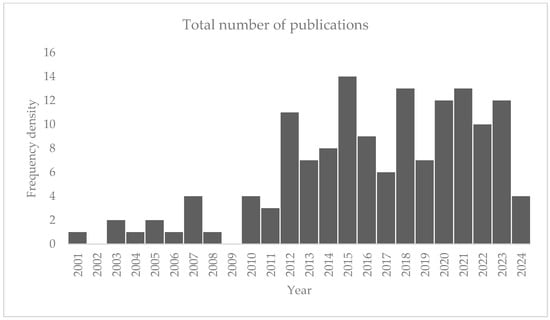
Figure 23.
Analysis of the profile of extracted sources.
With a value of 0.86, the distribution of extracted sources through Figure 24 demonstrates a favorable association between knowledge production in 2001 and 2024.
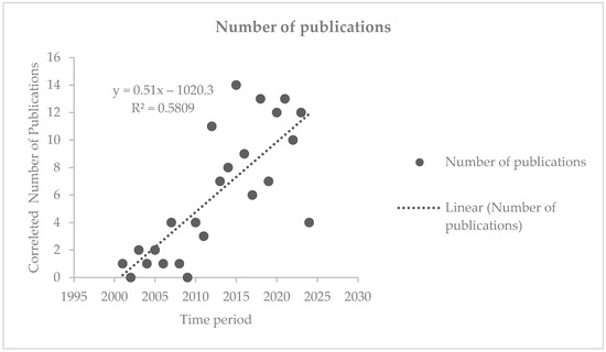
Figure 24.
Temporal correlation of the forecasting method’s assessed research sources in the publications this study found and examined.
The most common approach, according to the methods used, is advanced deep learning, which uses machine learning models with roughly 23% SLR, 19% hybrid models, 17% ANNs, 11% RK, 4% SVMs, 9% RF, 5% ARIMA, 4% GBMs, 4% LSTM, and 4% GPR, as shown in Figure 25.
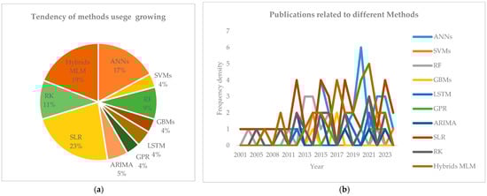
Figure 25.
Evaluation of the trend and exploratory performance of the various approaches in the extracted sources, with a focus on (a) biased and (b) quantitative.
The hybrid model’s method yields a preponderance of 145 bibliographic sources (Table 12). This is significantly greater than the estimated six sources utilizing SVM, GBMs, and GPR models, which give a comparatively lower number of explorations.
Table 12.
Comparison of the overall effectiveness and patterns of use of various techniques.
In a range of 6 and 33 cumulative extracted and processed sources, Figure 26 illustrates how the physical approaches and the traditional methods estimate the cumulative trend of higher use.
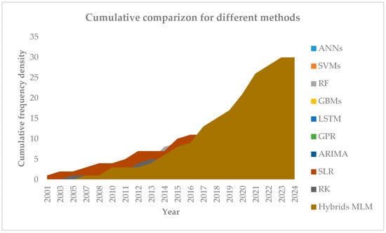
Figure 26.
In research on space-solar forecasting, the cumulative frequency of metrics consumption is reported.
4. A Discussion of Machine Learning Techniques for Parameterizing Solar Energy
Utilizing MLM that parametrizes solar radiation, the study enhanced solar irradiance mapping at high latitudes. In most cases, the model produced more accurate and precise results than those found in the input datasets, with a bias of 0.01 W/m2 and a lower error of 16.2 W/m2 [18]. Moreover, parameterization aids in the more accurate prediction of diffuse solar irradiation through multivariate regression and machine learning. Analogously, one might note that solar generation technologies can achieve significant market expansion by utilizing a specific amount of solar energy that coincides with a horizontal surface, increasing local grid penetration rates [3,200].
The primary ambiguity in the interpretation of the bibliographic sources accessed and analyzed was the inclusion of sources that comprehensively describe the model a priori in terms of parametric relationships to be considered, followed by a somatic analysis. This was primarily to meet the criteria for the summary of results using MLMs that reduce the risk of solar resource misuse. However, the sources use MLM to interpolate and/or anticipate solar energy and provide the parameters in terms of raw samples obtained by remote sensing or in situ measurement instruments (radiometers, photometers, etc.). For a summative analysis, MLMs have the advantage of standardizing the results on the same administrative scale and randomizing the results, which allows the output to be taken into account as a whole. The analysis of generalized parameters (direct and diffuse solar energy, which add up to the predicted global solar energy) brought on by the different atmospheric components (aerosols, water vapor, uniformly mixed gases, ozone layer, among others) is necessary to avoid the ambiguity this introduces into the sample analysis.
There is a significant advancement in estimates using neutral network loops and their variants but interpolated by the RF model, to occasionally fill in measurement gaps and/or measurement data of atmospheric parameters and/or solar energy. The summary and analysis of bibliographic sources reveal a wide range of uses for regression models, including SLR and RK, among others. This presents good analysis bias and lowers the risk of bias towards estimation errors.
The ozone transmittances for the years 2020 and 2021 differ significantly, yet the obtained numerical values are within 0.0098 of one another. The zenith angle and ozone concentration determine the biggest difference. Ozone has very little effect on overall transmittance because of its high transmittance. The water vapor transmittances compare quite well, with values that are around 0.9862 greater at zenithal angle zero. In addition to varying with the zenith angle, the discrepancies also change with the water vapor content.
The expected region data sample has strong variability, with a coefficient of dispersion of roughly 0.52. In contrast to clear and intermediate sky days, roughly 68% of intermediate sky days are mostly represented in the statistical data sample that was generated. This represents a rough statistical analysis of the initial data collected at a station, estimated at 70% of intermediate sky days. While this is in agreement with Kumler et al. (2018) [40], it also shows that short-term solar forecast models that rely only on global horizontal irradiance (GHI) measurements frequently fail to distinguish between factors that affect the GHI and those that can be accurately calculated by atmospheric models.
The time interval under examination and the number of inferred measurement stations shows a decorrelation, which becomes more pronounced for the anticipated values, both for the original GHI data sample that was inferred in situ and for the predicted GHI sample. The output of a solar plant is affected by the variability in solar energy, and this estimate is more pronounced on intermediate sky days, which can be the most problematic. Hoff and Perez (2010) [55] and Mucomole et al. (2024) [6] confirmed this result. These results are similarly consistent with those calculated by Mucomole et al. (2024) [6], but the estimated values tend to exhibit a high frequency of changes in the clear-sky index for their respective increments [15].
For a clean environment, the direct normal irradiances obtained for the two years are relatively similar when using the technique to account for aerosol attenuation; nevertheless, the spectrally integrated findings are very good at zenith angles less than 90°. The biggest difference that can exist between the two years is 0.0893. While the pattern is more configurable than previous models in that it can incorporate new observations to enhance the GHI prediction, if available, it does not require additional observations of different atmospheric parameters [3,40].
Almost identical findings are obtained at zenith angles less than 90° when the influence of turbidity is included, based on a visibility of 150 km. High diffuse multireflected solar energy is produced at bigger zenith angles due to some disagreement caused by albedo and the intensity of solar energy incidence [3,24,176].
The outcomes are more in line with the spectrally integrated approaches. The earlier finding was validated by similar comparisons made using various atmospheric factors. This improved the idealization’s accuracy, and using it is advised.
According to broadband simulations, the initial millimeters of precipitable water in the atmosphere absorb as much radiation as the next centimeters.
Whether the atmosphere is laden with water vapor or is dry, precipitable water produces results with roughly the same degree of error and remains virtually unaltered when the visibility parameter is adjusted. This finding helps to simplify the parameterization equation by assuming a constant volume of water vapor [94,155].
Because aerosol levels and gases can cause significant variations in ground-level solar resources, this study uses both observed and anticipated AOT to investigate the effects of different AOT forecast qualities on solar energy applications [201]. The findings are consistent with research that highlights the necessity of long-term projections for effective control and optimization of solar power systems, such as those published by Breitkreuz et al. (2009) [36] and Lauret et al. (2016) [34]. Local climatic parameters can be used to improve the approximation of the anticipated sample and machine learning models can be used to prepare for future calibrations [3,24,89].
The findings here improve the great PV system dimensioning by optimizing solar energy and solar plant output, hence sizing the PV system based on daily energy use. The evaluation is also a powerful tool for gauging environmental behavior in the context of climate change today. It can provide criteria for making decisions regarding the planning and execution of numerous projects in a variety of fields, including architecture, agriculture, fishing, medicine, aquaculture, and construction. When compared to other models previously mentioned, the results show that the actual quantity of predicted solar energy is around 1241.85 W/m2, taking into account all estimating parameters.
The combined data from all sources describe in detail how models are applied utilizing multiple sample sources, providing input of advancements in the use of MLM for parametric forecast analysis of solar energy. The physical effects of radiation scattering in the atmosphere, including the Rayleigh effect, MIE effect, and scattering by small, medium, and large aerosols, are among the parameters that are aggregated and taken into account in the model that is introduced.
However, future research can use a sample of hours of solar brightness and aggregate other physical effects of radiation interaction with matter to perform the same analysis instead of sampling in situ solar energy. This will allow for a more comprehensive understanding of the available solar resources and provide a different perspective on complexity. Nevertheless, an inference estimate of solar energy and the dynamics of the generalized cloud velocity as a whole can also be studied.
5. Summary and Conclusions
The idea of electrifying rural areas is associated with the use of clean sources, such as PV solar energy, which is efficient, clean, and oscillation-free. This type of energy has been gaining popularity worldwide, particularly in the study region of Mozambique, where access to electricity is scarce. Additionally, the installed PV power systems have a limited useful life due to various factors that interfere with their operation; the variability in solar energy is increasing. These factors are crucial for the planning and dependability of future PV electrical networks as well as other solar energy projects. It is feasible to synthesize and make the following deductions from the sample of scientific articles’ bibliographic data analyzed over the past 23 years, which was condensed into solar energy parametric forecast models validated with GHI samples gathered on location in specific areas.
There is a considerable propensity in the literature from the past five years to employ ANN and RF for solar forecasting, with a cumulative order of 28 and 14 sources. However, the SLR model tends to be used by RK, with 19 and 17 sources assessed, respectively. A cumulative analysis of the estimated solar energy using hybrid models from about 33 sources makes several inputs available for the final model summation, increasing the model’s viability and certainty while reducing forecast error.
The evenly mixed gases exhibit the least amount of attenuation based on the atmospheric factors utilized. The uniformly mixed gases, therefore, required the evaluation of a separate absorption term, which is unlimited and is ignored. When compared to gases that are evenly mixed, ozone attenuates slightly more. The amount of ozone in the atmosphere affects this. The three primary attenuators are aerosols, water vapor, and air molecule scattering. Hydrogen vapor and aerosols’ proportional relevance is contingent upon their atmospheric concentration. The simple scattering albedo, or w0, also affects aerosol absorptance. Regardless of the zenith angle, the transmittances of molecular absorbers are relatively constant. Significant reductions are observed in the Rayleigh and aerosol transmittances.
On clear days, the frequency density of the observation of values near zero is lower than that of values near one; on days with intermediate skies, the frequency density of the observation of values near one is lower than that of values near 0.66; on days with intermediate skies, the frequency density of the observation of values near one is lower than that of values near 0.020. In all cases, the analysis of the sky types shows that the clear sky index is similar to other days in that these values are within the theoretical radiation spectrum, which ranges from −1 to 1.
Owing to several factors that affect solar radiation as it approaches the Earth’s surface, the estimated measurement of solar energy variability offers a practical substitute for the current solar energy fluctuation. As a result, it is a crucial parameter to comprehend the true solar energy behavior from the perspective of future estimation. Still, the following is true: to obtain a more precise estimate, geographical features, atmospheric, climatic, and local influences are needed.
The GHI sample exhibits trends that are comparable to those of the in situ GHI sample, with the majority of the trends differing because cloud movement and meteorological factors will affect future trends. By correcting the real variation through even smaller scale measurements, the GHI’s degree of clarity can be raised.
The majority of the predicted and observed variability in GHI is explained by intermediate sky days, with a larger tendency for lower intermediate sky days. Over the examined spatiotemporal range, solar energy shows a considerable decorrelation, both in the anticipated GHI sample and on intermediate sky days. When machine-readable models are used to examine regression approaches, the prediction error is reduced, with RMSE verifying about 0.30 utilizing the RF model.
The evaluation of radiation in a specific bandwidth can be achieved by simply summing the spectral values. However, radiation over the whole solar spectrum can be calculated using the broadband approach, which is simply integrated over the whole solar spectrum.
6. Patents
This research article appears as one of the first obligations to attend to, in order to obtain a Doctorate degree, the Doctoral Course in Energy Science and Technology, at Eduardo Mondlane University, which the main author is attending.
Author Contributions
In this research article, the conceptualization, methodology, validation, and formal analysis, were conducted by F.V.M. and C.A.S.S.; the investigation, resources, data curation, writing, preparation of the original draft, writing, review and editing, acquisition of funding, visualization, and software were conducted by the main authors F.V.M., C.A.S.S. and L.L.M.; the supervision, project administration were conducted by F.V.M. and C.A.S.S.; the advanced curation of data, writing and supervision were conducted by F.V.M., C.A.S.S. and L.L.M. All authors have read and agreed to the published version of the manuscript.
Funding
This research was funded by CS–OGET, Faculty of Engineering, Eduardo Mondlane University, underfunding number CS-OGET/2023, for doctoral research.
Data Availability Statement
The data that back up the reported outcomes are accessible on the AERONET website at https://aeronet.gsfc.nasa.gov/new_web/webtool_aod_v3.html (accessed on 5 November 2023), NOAA website at https://www.noaa.gov/weather (accessed on 5 November 2023) and NASA POWER website https://power.larc.nasa.gov/data-access-viewer/ (accessed on 5 November 2023). Additional data that support the conclusions of this research have not been released and can be obtained from INAM [62], FUNAE [61], UEM [202], or by contacting the corresponding author.
Acknowledgments
We express our gratitude to the FUNAE, entities for their assistance in providing us with sample data from the campaign conducted between 2012 and 2014. We would also like to thank INAM for supplying us with the sample of solar radiation data spanning from 1995 to 2023, and for granting us access to their facilities for training and experimental tests. Additionally, we extend our appreciation to the Department of Physics at Eduardo Mondlane University for generously making their facilities available for real-time testing and measurements of the latest solar energy behavior. Their provision of a laboratory for data processing greatly contributed to the compilation of this research. Lastly, we would like to acknowledge CS-OGET for their support, as it played an integral role in the culmination stage of this doctoral research.
Conflicts of Interest
The authors declare no conflicts of interest.
References
- Hossain, R.; Ooa, A.M.T.; Alia, A.B.M.S. Historical Weather Data Supported Hybrid Renewable Energy Forecasting using Artificial Neural Network (ANN). Energy Procedia 2012, 14, 1035–1040. [Google Scholar] [CrossRef]
- Babar, B.; Luppino, L.T.; Boström, T.; Anfinsen, S.N. Random forest regression for improved mapping of solar irradiance at high latitudes. Sol. Energy 2020, 198, 81–92. [Google Scholar] [CrossRef]
- Iqbal, M. An Introduction to Solar Radiation; Academic Press: New York, NY, USA, 1983. [Google Scholar]
- Tsai, S.-B.; Xue, Y.; Zhang, J.; Chen, Q.; Liu, Y.; Zhou, J.; Dong, W. Models for forecasting growth trends in renewable energy. Renew. Sustain. Energy Rev. 2017, 77, 1169–1178. [Google Scholar] [CrossRef]
- Tracking SDG 7—The Energy Progress Report 2023. Available online: https://cdn.who.int/media/docs/default-source/air-pollution-documents/air-quality-and-health/sdg7-report2023-full-report_web.pdf?sfvrsn=669e8626_3&download=true (accessed on 16 December 2023).
- Mucomole, F.V.; Silva, C.A.S.; Magaia, L.L. Regressive and Spatio-Temporal Accessibility of Variability in Solar Energy on a Short Scale Measurement in the Southern and Mid Region of Mozambique. Energies 2024, 17, 2613. [Google Scholar] [CrossRef]
- Benghanem, M.; Joraid, A.A. A multiple correlation between different solar parameters in Medina, Saudi Arabia. Renew. Energy 2007, 32, 2424–2435. [Google Scholar] [CrossRef]
- Ohtake, H.; Shimose, K.; Fonseca, J.G.D.S.; Takashima, T.; Oozeki, T.; Yamada, Y. Accuracy of the solar irradiance forecasts of the Japan Meteorological Agency mesoscale model for the Kanto region, Japan. Sol. Energy 2013, 98, 138–152. [Google Scholar] [CrossRef]
- Mohanty, S.; Patra, P.K.; Sahoo, S.S.; Mohanty, A. Forecasting of solar energy with application for a growing economy like India: Survey and implication. Renew. Sustain. Energy Rev. 2017, 78, 539–553. [Google Scholar] [CrossRef]
- Zhang, P.; Ma, X.; She, K. Forecasting Japan’s Solar Energy Consumption Using a Novel Incomplete Gamma Grey Model. Sustainability 2019, 11, 5921. [Google Scholar] [CrossRef]
- Ramirez-Vergara, J.; Bosman, L.B.; Leon-Salas, W.D.; Wollega, E. Ambient temperature and solar irradiance forecasting prediction horizon sensitivity analysis. Mach. Learn. Appl. 2021, 6, 100128. [Google Scholar] [CrossRef]
- Sward, J.A.; Ault, T.R.; Zhang, K.M. Genetic algorithm selection of the weather research and forecasting model physics to support wind and solar energy integration. Energy 2022, 254, 124367. [Google Scholar] [CrossRef]
- Funk, P.A.; Larson, D.L. Parametric model of solar cooker performance. Sol. Energy 1998, 62, 63–68. [Google Scholar] [CrossRef]
- Sahin, G.; Isik, G.; van Sark, W.G.J.H.M. Predictive modeling of PV solar power plant efficiency considering weather conditions: A comparative analysis of artificial neural networks and multiple linear regression. Energy Rep. 2023, 10, 2837–2849. [Google Scholar] [CrossRef]
- Duf, J.A.; Beckman, W.A. Solar Engineering of Thermal Processes; Wiley: New York, NY, USA, 1980. [Google Scholar]
- Jawaid, F.; NazirJunejo, K. Predicting daily mean solar power using machine learning regression techniques. In Proceedings of the 2016 Sixth International Conference on Innovative Computing Technology (INTECH), Dublin, Ireland, 24–26 August 2016; pp. 355–360. [Google Scholar] [CrossRef]
- Litjens, G.B.M.A.; Kausika, B.B.; Worrell, E.; van Sark, W.G.J.H.M. A spatio-temporal city-scale assessment of residential photovoltaic power integration scenarios. Sol. Energy 2018, 174, 1185–1197. [Google Scholar] [CrossRef]
- Zhang, J.; Hodge, B.-M.; Lu, S.; Hamann, H.F.; Lehman, B.; Simmons, J.; Campos, E.; Banunarayanan, V.; Black, J.; Tedesco, J. Baseline and target values for regional and point PV power forecasts: Toward improved solar forecasting. Sol. Energy 2015, 122, 804–819. [Google Scholar] [CrossRef]
- Dyson, M.E.H.; Borgeson, S.D.; Tabone, M.D.; Callaway, D.S. Using smart meter data to estimate demand response potential, with application to solar energy integration. Energy Policy 2014, 73, 607–619. [Google Scholar] [CrossRef]
- Jebli, I.; Belouadha, F.-Z.; Kabbaj, M.I.; Tilioua, A. Prediction of solar energy guided by pearson correlation using machine learning. Energy 2021, 224, 120109. [Google Scholar] [CrossRef]
- Jung, Y.; Lee, H.; Kim, J.; Cho, Y.; Kim, J.; Lee, Y.G. Spatio-Temporal Characteristics in the Clearness Index Derived from Global Solar Radiation Observations in Korea. Atmosphere 2016, 7, 55. [Google Scholar] [CrossRef]
- Kaur, A.; Nonnenmacher, L.; Pedro, H.T.C.; Coimbra, C.F.M. Benefits of solar forecasting for energy imbalance markets. Renew. Energy 2016, 86, 819–830. [Google Scholar] [CrossRef]
- Zhang, J.; Florita, A.; Hodge, B.-M.; Lu, S.; Hamann, H.F.; Banunarayanan, V.; Brockway, A.M. A suite of metrics for assessing the performance of solar power forecasting. Sol. Energy 2015, 111, 157–175. [Google Scholar] [CrossRef]
- Wenham, S.R.; Green, M.A.; Watt, M.E.; Corkish, R.; Sproul, A. (Eds.) Applied Photovoltaics, 3rd ed.; Routledge: London, UK, 2011. [Google Scholar] [CrossRef]
- Mucomole, F.V.; Silva, C.A.S.; Magaia, L.L. Temporal Variability of Solar Energy Availability in the Conditions of the Southern Region of Mozambique. Am. J. Energy Nat. Resour. 2023, 2, 27–50. [Google Scholar] [CrossRef]
- Energy Access Situation in Mozambique—Energypedia. Available online: https://energypedia.info/wiki/Situa%C3%A7%C3%A3o_de_Acesso_%C3%A0_Energia_em_Mo%C3%A7ambique (accessed on 15 December 2023).
- Yousif, J.H.; Al-Balushi, H.A.; Kazem, H.A.; Chaichan, M.T. Analysis and forecasting of weather conditions in Oman for renewable energy applications. Case Stud. Therm. Eng. 2019, 13, 100355. [Google Scholar] [CrossRef]
- Qing, X.; Niu, Y. Hourly day-ahead solar irradiance prediction using weather forecasts by LSTM. Energy 2018, 148, 461–468. [Google Scholar] [CrossRef]
- Adedeji, P.A.; Akinlabi, S.A.; Madushele, N.; Olatunji, O.O. Neuro-fuzzy resource forecast in site suitability assessment for wind and solar energy: A mini review. J. Clean. Prod. 2020, 269, 122104. [Google Scholar] [CrossRef]
- Pedro, H.T.C.; Inman, R.H.; Coimbra, C.F.M. 4—Mathematical methods for optimized solar forecasting. In Renewable Energy Forecasting; Kariniotakis, G., Ed.; Woodhead Publishing Series in Energy; Woodhead Publishing: Sawston, UK, 2017; pp. 111–152. [Google Scholar] [CrossRef]
- Choi, M.; Rachunok, B.; Nateghi, R. Short-term solar irradiance forecasting using convolutional neural networks and cloud imagery. Environ. Res. Lett. 2021, 16, 044045. [Google Scholar] [CrossRef]
- Mellit, A.; Pavan, A.M. A 24-h forecast of solar irradiance using artificial neural network: Application for performance prediction of a grid-connected PV plant at Trieste, Italy. Sol. Energy 2010, 84, 807–821. [Google Scholar] [CrossRef]
- Ozoegwu, C.G. Artificial neural network forecast of monthly mean daily global solar radiation of selected locations based on time series and month number. J. Clean. Prod. 2019, 216, 1–13. [Google Scholar] [CrossRef]
- Lauret, P.; Lorenz, E.; David, M. Solar Forecasting in a Challenging Insular Context. Atmosphere 2016, 7, 18. [Google Scholar] [CrossRef]
- Wen, H.; Du, Y.; Chen, X.; Lim, E.G.; Wen, H.; Yan, K. A regional solar forecasting approach using generative adversarial networks with solar irradiance maps. Renew. Energy 2023, 216, 119043. [Google Scholar] [CrossRef]
- Breitkreuz, H.; Schroedter-Homscheidt, M.; Holzer-Popp, T.; Dech, S. Short-Range Direct and Diffuse Irradiance Forecasts for Solar Energy Applications Based on Aerosol Chemical Transport and Numerical Weather Modeling. J. Appl. Meteorol. Climatol. 2009, 48, 1766–1779. [Google Scholar] [CrossRef]
- Boland, J.; David, M.; Lauret, P. Short term solar radiation forecasting: Island versus continental sites. Energy 2016, 113, 186–192. [Google Scholar] [CrossRef]
- Blaga, R.; Sabadus, A.; Stefu, N.; Dughir, C.; Paulescu, M.; Badescu, V. A current perspective on the accuracy of incoming solar energy forecasting. Prog. Energy Combust. Sci. 2019, 70, 119–144. [Google Scholar] [CrossRef]
- Nam, S.; Hur, J. A hybrid spatio-temporal forecasting of solar generating resources for grid integration. Energy 2019, 177, 503–510. [Google Scholar] [CrossRef]
- Kumler, A.; Xie, Y.; Zhang, Y. A New Approach for Short-Term Solar Radiation Forecasting Using the Estimation of Cloud Fraction and Cloud Albedo; NREL: Golden, CO, USA, 2018. [Google Scholar] [CrossRef]
- Aler, R.; Martín, R.; Valls, J.M.; Galván, I.M. A Study of Machine Learning Techniques for Daily Solar Energy Forecasting Using Numerical Weather Models. In Intelligent Distributed Computing VIII; Camacho, D., Braubach, L., Venticinque, S., Badica, C., Eds.; Springer International Publishing: Cham, Switzerland, 2015; pp. 269–278. [Google Scholar]
- Dhillon, S.; Madhu, C.; Kaur, D.; Singh, S. A Solar Energy Forecast Model Using Neural Networks: Application for Prediction of Power for Wireless Sensor Networks in Precision Agriculture. Wirel. Pers. Commun. 2020, 112, 2741–2760. [Google Scholar] [CrossRef]
- Ramirez Camargo, L.; Zink, R.; Dorner, W.; Stoeglehner, G. Spatio-temporal modeling of roof-top photovoltaic panels for improved technical potential assessment and electricity peak load offsetting at the municipal scale. Comput. Environ. Urban Syst. 2015, 52, 58–69. [Google Scholar] [CrossRef]
- Saffaripour, M.H.; Mehrabian, M.A.; Bazargan, H. Predicting solar radiation fluxes for solar energy system applications. Int. J. Environ. Sci. Technol. 2013, 10, 761–768. [Google Scholar] [CrossRef]
- McCandless, T.; Jiménez, P.A. Examining the Potential of a Random Forest Derived Cloud Mask from GOES-R Satellites to Improve Solar Irradiance Forecasting. Energies 2020, 13, 1671. [Google Scholar] [CrossRef] [PubMed]
- Anuradha, K.; Erlapally, D.; Karuna, G.; Srilakshmi, V.; Adilakshmi, K. Analysis of Solar Power Generation Forecasting Using Machine Learning Techniques. E3S Web Conf. 2021, 309, 01163. [Google Scholar] [CrossRef]
- Zagouras, A.; Pedro, H.T.C.; Coimbra, C.F.M. On the role of lagged exogenous variables and spatio–temporal correlations in improving the accuracy of solar forecasting methods. Renew. Energy 2015, 78, 203–218. [Google Scholar] [CrossRef]
- Yang, D.; Alessandrini, S. An ultra-fast way of searching weather analogs for renewable energy forecasting. Sol. Energy 2019, 185, 255–261. [Google Scholar] [CrossRef]
- Arumugham, D.R.; Rajendran, P. Modelling global solar irradiance for any location on earth through regression analysis using high-resolution data. Renew. Energy 2021, 180, 1114–1123. [Google Scholar] [CrossRef]
- Ahmad, M.W.; Reynolds, J.; Rezgui, Y. Predictive modelling for solar thermal energy systems: A comparison of support vector regression, random forest, extra trees and regression trees. J. Clean. Prod. 2018, 203, 810–821. [Google Scholar] [CrossRef]
- Portabella, M.; Stoffelen, A. Scatterometer Backscatter Uncertainty Due to Wind Variability. IEEE Trans. Geosci. Remote Sens. 2006, 44, 3356–3362. [Google Scholar] [CrossRef]
- Cerralbo, P.; Grifoll, M.; Moré, J.; Bravo, M.; Sairouní Afif, A.; Espino, M. Wind variability in a coastal area (Alfacs Bay, Ebro River delta). Adv. Sci. Res. 2015, 12, 11–21. [Google Scholar] [CrossRef]
- Munkhammar, J. Very short-term probabilistic and scenario-based forecasting of solar irradiance using Markov-chain mixture distribution modeling. Sol. Energy Adv. 2024, 4, 100057. [Google Scholar] [CrossRef]
- Kumar, D. Hyper-temporal variability analysis of solar insolation with respect to local seasons. Remote Sens. Appl. Soc. Environ. 2019, 15, 100241. [Google Scholar] [CrossRef]
- Hoff, T.E.; Perez, R. Quantifying PV power Output Variability. Sol. Energy 2010, 84, 1782–1793. [Google Scholar] [CrossRef]
- Mucomole, F.V.; Silva, C.S.A.; Magaia, L.L. Quantifying the Variability of Solar Energy Fluctuations at High–Frequencies through Short-Scale Measurements in the East–Channel of Mozambique Conditions. Am. J. Energy Nat. Resour. 2024, 3, 21–40. [Google Scholar] [CrossRef]
- Paulescu, M.; Paulescu, E. Short-term forecasting of solar irradiance. Renew. Energy 2019, 143, 985–994. [Google Scholar] [CrossRef]
- Gutierrez-Corea, F.-V.; Manso-Callejo, M.-A.; Moreno-Regidor, M.-P.; Velasco-Gómez, J. Spatial Estimation of Sub-Hour Global Horizontal Irradiance Based on Official Observations and Remote Sensors. Sensors 2014, 14, 6758–6787. [Google Scholar] [CrossRef] [PubMed]
- Wang, L.; Gong, W.; Hu, B.; Lin, A.; Li, H.; Zou, L. Modeling and analysis of the spatiotemporal variations of photosynthetically active radiation in China during 1961–2012. Renew. Sustain. Energy Rev. 2015, 49, 1019–1032. [Google Scholar] [CrossRef]
- Page, M.J.; McKenzie, J.E.; Bossuyt, P.M.; Boutron, I.; Hoffmann, T.C.; Mulrow, C.D.; Shamseer, L.; Tetzlaff, J.M.; Akl, E.A.; Brennan, S.E.; et al. The PRISMA 2020 statement: An updated guideline for reporting systematic reviews. Syst. Rev. 2021, 10, 89. [Google Scholar] [CrossRef] [PubMed]
- FUNAE (National Energy Fund of Mozambique) [Online]. 2023. Available online: https://funae.co.mz/ (accessed on 30 April 2023).
- INAM (National Meteorology Institute of Mozambique) [Online]. 2024. Available online: https://www.inam.gov.mz/index.php/pt/ (accessed on 5 May 2023).
- AERONET (Aerosol Robotic Network) [Online]. 2024. Available online: https://aeronet.gsfc.nasa.gov/ (accessed on 12 February 2023).
- Smith, C.J.; Bright, J.M.; Crook, R. Cloud cover effect of clear-sky index distributions and differences between human and automatic cloud observations. Sol. Energy 2017, 144, 10–21. [Google Scholar] [CrossRef]
- Kurniadi, A.P.; Aimon, H.; Salim, Z.; Ragimun, R.; Sonjaya, A.; Setiawan, S.; Siagian, V.; Nasution, L.Z.; Nurhidajat, R.; Mutaqin, M.; et al. Analysis of Existing and Forecasting for Coal and Solar Energy Consumption on Climate Change in Asia Pacific: New Evidence for Sustainable Development Goals. Int. J. Energy Econ. Policy 2024, 14, 352–359. [Google Scholar] [CrossRef]
- Renkema, Y.; Visser, L.; AlSkaif, T. Enhancing the reliability of probabilistic PV power forecasts using conformal prediction. Sol. Energy Adv. 2024, 4, 100059. [Google Scholar] [CrossRef]
- Arslan, H.; Baltaci, H.; Akkoyunlu, B.O.; Karanfil, S.; Tayanc, M. Wind speed variability and wind power potential over Turkey: Case studies for Çanakkale and İstanbul. Renew. Energy 2020, 145, 1020–1032. [Google Scholar] [CrossRef]
- Vindel, J.M.; Valenzuela, R.X.; Navarro, A.A.; Polo, J. Temporal and spatial variability analysis of the solar radiation in a region affected by the intertropical convergence zone. Meteorol. Appl. 2020, 27, e1824. [Google Scholar] [CrossRef]
- Klein, S.A.; Cooper, P.I.; Freeman, T.L.; Beekman, D.M.; Beckman, W.A.; Duffie, J.A. A method of simulation of solar processes and its application. Sol. Energy 1975, 17, 29–37. [Google Scholar] [CrossRef]
- Charles, R.G.; Davies, M.L.; Douglas, P.; Hallin, I.L.; Mabbett, I. Sustainable energy storage for solar home systems in rural Sub-Saharan Africa—A comparative examination of lifecycle aspects of battery technologies for circular economy, with emphasis on the South African context. Energy 2019, 166, 1207–1215. [Google Scholar] [CrossRef]
- Puga-Gil, D.; Astray, G.; Barreiro, E.; Gálvez, J.F.; Mejuto, J.C. Global Solar Irradiation Modelling and Prediction Using Machine Learning Models for Their Potential Use in Renewable Energy Applications. Mathematics 2022, 10, 4746. [Google Scholar] [CrossRef]
- Lichtenwoehrer, P.; Abart-Heriszt, L.; Kretschmer, F.; Suppan, F.; Stoeglehner, G.; Neugebauer, G. Evaluating Spatial Interdependencies of Sector Coupling Using Spatiotemporal Modelling. Energies 2021, 14, 1256. [Google Scholar] [CrossRef]
- Ghayekhloo, M.; Ghofrani, M.; Menhaj, M.B.; Azimi, R. A novel clustering approach for short-term solar radiation forecasting. Sol. Energy 2015, 122, 1371–1383. [Google Scholar] [CrossRef]
- Ibrahim, S.; Daut, I.; Irwan, Y.M.; Irwanto, M.; Gomesh, N.; Farhana, Z. Linear Regression Model in Estimating Solar Radiation in Perlis. Energy Procedia 2012, 18, 1402–1412. [Google Scholar] [CrossRef]
- Twidell, J.; Weir, T. Renewable Energy Resources, 3rd ed.; Routledge: London, UK, 2015. [Google Scholar] [CrossRef]
- Mei, L.L.; Xue, Y.; Kokhanovsky, A.A.; von Hoyningen-Huene, W.; de Leeuw, G.; Burrows, J.P. Retrieval of aerosol optical depth over land surfaces from AVHRR data. Atmos. Meas. Techol. 2014, 7, 2411–2420. [Google Scholar] [CrossRef]
- Zhang, W.; Xu, H.; Zheng, F. Aerosol Optical Depth Retrieval over East Asia Using Himawari-8/AHI Data. Remote Sens. 2018, 10, 137. [Google Scholar] [CrossRef]
- Mishra, M.K. Retrieval of Aerosol Optical Depth From INSAT-3D Imager Over Asian Landmass and Adjoining Ocean: Retrieval Uncertainty and Validation. J. Geophys. Res. Atmos. 2018, 123, 5484–5508. [Google Scholar] [CrossRef]
- Levy, R.C.; Munchak, L.A.; Mattoo, S.; Patadia, F.; Remer, L.A.; Holz, R.E. Towards a long-term global aerosol optical depth record: Applying a consistent aerosol retrieval algorithm to MODIS and VIIRS-observed reflectance. Atmos. Meas. Technol. 2015, 8, 4083–4110. [Google Scholar] [CrossRef]
- Zhang, H.; Lyapustin, A.; Wang, Y.; Kondragunta, S.; Laszlo, I.; Ciren, P.; Hoff, R.M. A multi-angle aerosol optical depth retrieval algorithm for geostationary satellite data over the United States. Atmos. Chem. Phys. 2011, 11, 11977–11991. [Google Scholar] [CrossRef]
- Pedro, H.T.C.; Coimbra, C.F.M. Assessment of forecasting techniques for solar power production with no exogenous inputs. Sol. Energy 2012, 86, 2017–2028. [Google Scholar] [CrossRef]
- Gupta, P.; Levy, R.C.; Mattoo, S.; Remer, L.A.; Munchak, L.A. A surface reflectance scheme for retrieving aerosol optical depth over urban surfaces in MODIS Dark Target retrieval algorithm. Atmos. Meas. Technol. 2016, 9, 3293–3308. [Google Scholar] [CrossRef]
- Sun, L.; Wei, J.; Bilal, M.; Tian, X.; Jia, C.; Guo, Y.; Mi, X. Aerosol Optical Depth Retrieval over Bright Areas Using Landsat 8 OLI Images. Remote Sens. 2016, 8, 23. [Google Scholar] [CrossRef]
- Krishnan, N.; Kumar, K.R.; Inda, C.S. How solar radiation forecasting impacts the utilization of solar energy: A critical review. J. Clean. Prod. 2023, 388, 135860. [Google Scholar] [CrossRef]
- Tian, X.; Liu, S.; Sun, L.; Liu, Q. Retrieval of Aerosol Optical Depth in the Arid or Semiarid Region of Northern Xinjiang, China. Remote Sens. 2018, 10, 197. [Google Scholar] [CrossRef]
- Gopinathan, K.K. A simple method for predicting global solar radiation on a horizontal surface. Sol. Wind Technol. 1988, 5, 581–583. [Google Scholar] [CrossRef]
- Badescu, V.; Budea, S. How significant is the stability of the radiative regime when the best operation of solar DHW systems is evaluated? Renew. Energy 2016, 88, 346–358. [Google Scholar] [CrossRef]
- Chen, Y.; Yang, S.; Qian, Y. Big data analysis of solar energy fluctuation characteristics and integration of wind-photovoltaic to hydrogen system. In Computer Aided Chemical Engineering; Kokossis, A.C., Georgiadis, M.C., Pistikopoulos, E., Eds.; 33 European Symposium on Computer Aided Process Engineering; Elsevier: Amsterdam, The Netherlands, 2023; Volume 52, pp. 3103–3109. [Google Scholar] [CrossRef]
- Kómar, L.; Kocifaj, M. Uncertainty of daylight illuminance on vertical building façades when determined from sky scanner data: A numerical study. Sol. Energy 2014, 110, 15–21. [Google Scholar] [CrossRef]
- Mustafa, M.; Malik, M.O.F. Factors Hindering Solar Photovoltaic System Implementation in Buildings and Infrastructure Projects: Analysis through a Multiple Linear Regression Model and Rule-Based Decision Support System. Buildings 2023, 13, 1786. [Google Scholar] [CrossRef]
- Ramedani, Z.; Omid, M.; Keyhani, A.; Khoshnevisan, B.; Saboohi, H. A comparative study between fuzzy linear regression and support vector regression for global solar radiation prediction in Iran. Sol. Energy 2014, 109, 135–143. [Google Scholar] [CrossRef]
- Fahrmeir, L.; Kneib, T.; Lang, S.; Marx, B. Regression: Models, Methods and Applications; Springer: Berlin/Heidelberg, Germany, 2013. [Google Scholar] [CrossRef]
- Jogunuri, S.; Ft, J.; Stonier, A.A.; Peter, G.; Jayaraj, J.; Ganji, V. Random Forest machine learning algorithm based seasonal multi-step ahead short-term solar photovoltaic power output forecasting. In IET Renewable Power Generation; Wiley: Hoboken, NJ, USA, 2024. [Google Scholar] [CrossRef]
- Perveen, G.; Rizwan, M.; Goel, N.; Anand, P. Artificial neural network models for global solar energy and photovoltaic power forecasting over India. Energy Sources Part Recovery Util. Environ. Eff. 2020, 47, 864–889. [Google Scholar] [CrossRef]
- Wu, J.; Niu, Z.; Li, X.; Huang, L.; Nielsen, P.S.; Liu, X. Understanding multi-scale spatiotemporal energy consumption data: A visual analysis approach. Energy 2023, 263, 125939. [Google Scholar] [CrossRef]
- Alzahrani, A.; Shamsi, P.; Dagli, C.; Ferdowsi, M. Solar Irradiance Forecasting Using Deep Neural Networks. Procedia Comput. Sci. 2017, 114, 304–313. [Google Scholar] [CrossRef]
- Ayet, A.; Tandeo, P. Nowcasting solar irradiance using an analog method and geostationary satellite images. Sol. Energy 2018, 164, 301–315. [Google Scholar] [CrossRef]
- Barhmi, K.; Heynen, C.; Golroodbari, S.; van Sark, W. A Review of Solar Forecasting Techniques and the Role of Artificial Intelligence. Solar 2024, 4, 99–135. [Google Scholar] [CrossRef]
- Zolfaghari, M.; Golabi, M.R. Modeling and predicting the electricity production in hydropower using conjunction of wavelet transform, long short-term memory and random forest models. Renew. Energy 2021, 170, 1367–1381. [Google Scholar] [CrossRef]
- Nielsen, M.A. Neural Networks and Deep Learning; Determination Press: San Francisco, CA, USA, 2015; Available online: http://neuralnetworksanddeeplearning.com (accessed on 12 June 2024).
- Pizarroso, J.; Portela, J.; Muñoz, A. NeuralSens: Sensitivity Analysis of Neural Networks. J. Stat. Softw. 2022, 102, 1–36. [Google Scholar] [CrossRef]
- Bergmeir, C.; Benítez, J.M. Neural Networks in R Using the Stuttgart Neural Network Simulator: RSNNS. J. Stat. Softw. 2012, 46, 1–26. [Google Scholar] [CrossRef]
- Beck, M.W. NeuralNetTools: Visualization and Analysis Tools for Neural Networks. J. Stat. Softw. 2018, 85, 1–20. [Google Scholar] [CrossRef] [PubMed]
- Tso, G.K.F.; Yau, K.K.W. Predicting electricity energy consumption: A comparison of regression analysis, decision tree and neural networks. Energy 2007, 32, 1761–1768. [Google Scholar] [CrossRef]
- Amrouche, B.; Le Pivert, X. Artificial neural network based daily local forecasting for global solar radiation. Appl. Energy 2014, 130, 333–341. [Google Scholar] [CrossRef]
- Dahmani, K.; Notton, G.; Voyant, C.; Dizene, R.; Nivet, M.L.; Paoli, C.; Tamas, W. Multilayer Perceptron approach for estimating 5-min and hourly horizontal global irradiation from exogenous meteorological data in locations without solar measurements. Renew. Energy 2016, 90, 267–282. [Google Scholar] [CrossRef]
- Sridharan, M. Generalized Regression Neural Network Model Based Estimation of Global Solar Energy Using Meteorological Parameters. Ann. Data Sci. 2023, 10, 1107–1125. [Google Scholar] [CrossRef]
- Flocas, A.A. Estimation and prediction of global solar radiation over Greece. Sol. Energy 1980, 24, 63–70. [Google Scholar] [CrossRef]
- Panamtash, H.; Zhou, Q.; Hong, T.; Qu, Z.; Davis, K.O. A copula-based Bayesian method for probabilistic solar power forecasting. Sol. Energy 2020, 196, 336–345. [Google Scholar] [CrossRef]
- Sun, H.; Gui, D.; Yan, B.; Liu, Y.; Liao, W.; Zhu, Y.; Lu, C.; Zhao, N. Assessing the potential of random forest method for estimating solar radiation using air pollution index. Energy Convers. Manag. 2016, 119, 121–129. [Google Scholar] [CrossRef]
- Kuo, P.-H.; Huang, C.-J. A Green Energy Application in Energy Management Systems by an Artificial Intelligence-Based Solar Radiation Forecasting Model. Energies 2018, 11, 819. [Google Scholar] [CrossRef]
- Mathiesen, P.; Collier, C.; Kleissl, J. A high-resolution, cloud-assimilating numerical weather prediction model for solar irradiance forecasting. Sol. Energy 2013, 92, 47–61. [Google Scholar] [CrossRef]
- Devaraj, J.; Madurai Elavarasan, R.; Shafiullah, G.; Jamal, T.; Khan, I. A holistic review on energy forecasting using big data and deep learning models. Int. J. Energy Res. 2021, 45, 13489–13530. [Google Scholar] [CrossRef]
- Ramsami, P.; Oree, V. A hybrid method for forecasting the energy output of photovoltaic systems. Energy Convers. Manag. 2015, 95, 406–413. [Google Scholar] [CrossRef]
- Gupta, S.; Katta, A.R.; Baldaniya, Y.; Kumar, R. Hybrid Random Forest and Particle Swarm Optimization Algorithm for Solar Radiation Prediction. In Proceedings of the 2020 IEEE 5th International Conference on Computing Communication and Automation (ICCCA), Greater Noida, India, 30–31 October 2020; pp. 302–307. [Google Scholar] [CrossRef]
- Travieso-González, C.M.; Cabrera-Quintero, F.; Piñán-Roescher, A.; Celada-Bernal, S. A Review and Evaluation of the State of Art in Image-Based Solar Energy Forecasting: The Methodology and Technology Used. Appl. Sci. 2024, 14, 5605. [Google Scholar] [CrossRef]
- Erdener, B.C.; Feng, C.; Doubleday, K.; Florita, A.; Hodge, B.-M. A review of behind-the-meter solar forecasting. Renew. Sustain. Energy Rev. 2022, 160, 112224. [Google Scholar] [CrossRef]
- Sharma, A.; Kakkar, A. A review on solar forecasting and power management approaches for energy-harvesting wireless sensor networks. Int. J. Commun. Syst. 2020, 33, e4366. [Google Scholar] [CrossRef]
- Zhang, Y.; Shen, Y.; Xia, X.; Shi, G. Validation of GFS day-ahead solar irradiance forecasts in China. arXiv 2020, arXiv:2007.01639. [Google Scholar]
- Hill, A.; Massey, A.; Mandallaz, D. The R Package forestinventory: Design-Based Global and Small Area Estimations for Multiphase Forest Inventories. J. Stat. Softw. 2021, 97, 1–40. [Google Scholar] [CrossRef]
- Kuiper, R.M.; Hoijtink, H. A Fortran 90 Program for the Generalized Order-Restricted Information Criterion. J. Stat. Softw. 2013, 54, 1–19. [Google Scholar] [CrossRef]
- Fu, C.-L.; Cheng, H.-Y. Predicting solar irradiance with all-sky image features via regression. Sol. Energy 2013, 97, 537–550. [Google Scholar] [CrossRef]
- Yagli, G.M.; Yang, D.; Srinivasan, D. Reconciling solar forecasts: Sequential reconciliation. Sol. Energy 2019, 179, 391–397. [Google Scholar] [CrossRef]
- Kühn, M.; Nakaten, N.; Streibel, M.; Kempka, T. CO2 Geological Storage and Utilization for a Carbon Neutral “Power-to-gas-to-power” Cycle to Even Out Fluctuations of Renewable Energy Provision. Energy Procedia 2014, 63, 8044–8049. [Google Scholar] [CrossRef]
- Zwane, N.; Tazvinga, H.; Botai, C.; Murambadoro, M.; Botai, J.; de Wit, J.; Mabasa, B.; Daniel, S.; Mabhaudhi, T. A Bibliometric Analysis of Solar Energy Forecasting Studies in Africa. Energies 2022, 15, 5520. [Google Scholar] [CrossRef]
- Yang, C.; Xie, L. A novel ARX-based multi-scale spatio-temporal solar power forecast model. In Proceedings of the 2012 North American Power Symposium (NAPS), Champaign, IL, USA, 9–11 September 2012; pp. 1–6. [Google Scholar] [CrossRef]
- Tawn, R.; Browell, J. A review of very short-term wind and solar power forecasting. Renew. Sustain. Energy Rev. 2022, 153, 111758. [Google Scholar] [CrossRef]
- Smith, P.F.; Ganesh, S.; Liu, P. A comparison of random forest regression and multiple linear regression for prediction in neuroscience. J. Neurosci. Methods 2013, 220, 85–91. [Google Scholar] [CrossRef]
- Liu, D.; Sun, K. Random forest solar power forecast based on classification optimization. Energy 2019, 187, 115940. [Google Scholar] [CrossRef]
- Breiman, L. Random Forests. Mach. Learn. 2001, 45, 5–32. [Google Scholar] [CrossRef]
- Perpiñán, O.; Marcos, J.; Lorenzo, E. Electrical power fluctuations in a network of DC/AC inverters in a large PV plant: Relationship between correlation, distance and time scale. Sol. Energy 2013, 88, 227–241. [Google Scholar] [CrossRef]
- Klima, K.; Apt, J. Geographic smoothing of solar PV: Results from Gujarat. Environ. Res. Lett. 2015, 10, 104001. [Google Scholar] [CrossRef]
- Perez, R.; David, M.; Hoff, T.E.; Jamaly, M.; Kivalov, S.; Kleissl, J.; Lauret, P.; Perez, M. Spatial and Temporal Variability of Solar Energy. Found. Trends® Renew. Energy 2016, 1, 1–44. [Google Scholar] [CrossRef]
- Marcos, J.; Marroyo, L.; Lorenzo, E.; Alvira, D.; Izco, E. Power output fluctuations in large scale pv plants: One year observations with one second resolution and a derived analytic model: Power Output Fluctuations in Large Scale PV plants. Prog. Photovolt. Res. Appl. 2011, 19, 218–227. [Google Scholar] [CrossRef]
- Mills, A. Understanding Variability and Uncertainty of Photovoltaics for Integration with the Electric Power System; LBNL-2855E; Lawrence Berkeley National Laboratory: Berkeley, CA, USA, 2019; Available online: https://escholarship.org/uc/item/58z9s527 (accessed on 15 May 2023).
- Arias-Castro, E.; Kleissl, J.; Lave, M. A Poisson model for anisotropic solar ramp rate correlations. Sol. Energy 2014, 101, 192–202. [Google Scholar] [CrossRef]
- Halász, G.; Malachi, Y. Solar energy from Negev desert, Israel: Assessment of power fluctuations for future PV fleet. Energy Sustain. Dev. 2014, 21, 20–29. [Google Scholar] [CrossRef]
- Madeh Piryonesi, S.; El-Diraby, T.E. Using Machine Learning to Examine Impact of Type of Performance Indicator on Flexible Pavement Deterioration Modeling. J. Infrastruct. Syst. 2021, 27, 04021005. [Google Scholar] [CrossRef]
- Didavi, A.B.K.; Agbokpanzo, R.G.; Agbomahena, M. Comparative study of Decision Tree, Random Forest and XGBoost performance in forecasting the power output of a photovoltaic system. In Proceedings of the 2021 4th International Conference on Bio-Engineering for Smart Technologies (BioSMART), Paris/Créteil, France, 8–10 December 2021; pp. 1–5. [Google Scholar] [CrossRef]
- Grantham, A.; Gel, Y.R.; Boland, J. Nonparametric short-term probabilistic forecasting for solar radiation. Sol. Energy 2016, 133, 465–475. [Google Scholar] [CrossRef]
- Srivastava, R.; Tiwari, A.N.; Giri, V.K. Solar radiation forecasting using MARS, CART, M5, and random forest model: A case study for India. Heliyon 2019, 5, e02692. [Google Scholar] [CrossRef]
- Madanchi, A.; Absalan, M.; Lohmann, G.; Anvari, M.; Reza Rahimi Tabar, M. Strong short-term non-linearity of solar irradiance fluctuations. Sol. Energy 2017, 144, 1–9. [Google Scholar] [CrossRef]
- Woyte, A.; Belmans, R.; Nijs, J. Fluctuations in instantaneous clearness index: Analysis and statistics. Sol. Energy 2007, 81, 195–206. [Google Scholar] [CrossRef]
- Jung, Y.; Jung, J.; Kim, B.; Han, S. Long short-term memory recurrent neural network for modeling temporal patterns in long-term power forecasting for solar PV facilities: Case study of South Korea. J. Clean. Prod. 2020, 250, 119476. [Google Scholar] [CrossRef]
- Kumari, P.; Toshniwal, D. Long short term memory–convolutional neural network based deep hybrid approach for solar irradiance forecasting. Appl. Energy 2021, 295, 117061. [Google Scholar] [CrossRef]
- Kamani, D.; Ardehali, M.M. Long-term forecast of electrical energy consumption with considerations for solar and wind energy sources. Energy 2023, 268, 126617. [Google Scholar] [CrossRef]
- Sopian, K.; Othman, M.Y.H. Estimates of monthly average daily global solar radiation in Malaysia. Renew. Energy 1992, 2, 319–325. [Google Scholar] [CrossRef]
- Kayima, P.; Semakula, H.M.; Wasswa, H.; Mugagga, F.; Mukwaya, P.I. Analysis of the socio-economic benefits of on-grid hybrid solar energy system on Bugala island in Uganda. Energy Sustain. Dev. 2023, 77, 101332. [Google Scholar] [CrossRef]
- Stevović, I.; Mirjanić, D.; Stevović, S. Possibilities for wider investment in solar energy implementation. Energy 2019, 180, 495–510. [Google Scholar] [CrossRef]
- Alkasassbeh, M. Hybrid One-Step Block Fourth Derivative Method for the Direct Solution of Third Order Initial Value Problems of Ordinary Differential Equations. Int. J. Pure Appl. Math. 2018, 119, 207–224. Available online: https://www.academia.edu/79478316/Hybrid_One_Step_Block_Fourth_Derivative_Method_for_the_Direct_Solution_of_Third_Order_Initial_Value_Problems_of_Ordinary_Differential_Equations (accessed on 7 July 2024).
- Aslam, S.; Herodotou, H.; Mohsin, S.M.; Javaid, N.; Ashraf, N.; Aslam, S. A survey on deep learning methods for power load and renewable energy forecasting in smart microgrids. Renew. Sustain. Energy Rev. 2021, 144, 110992. [Google Scholar] [CrossRef]
- Kurtgoz, Y.; Deniz, E. Chapter 1.8—Comparison of ANN, Regression Analysis, and ANFIS Models in Estimation of Global Solar Radiation for Different Climatological Locations. In Exergetic, Energetic and Environmental Dimensions; Dincer, I., Colpan, C.O., Kizilkan, O., Eds.; Academic Press: Cambridge, MA, USA, 2018; pp. 133–148. [Google Scholar] [CrossRef]
- Kumar, D.S.; Maharjan, S.; Albert; Srinivasan, D. Ramp-rate limiting strategies to alleviate the impact of PV power ramping on voltage fluctuations using energy storage systems. Sol. Energy 2022, 234, 377–386. [Google Scholar] [CrossRef]
- Deo, R.C.; Wen, X.; Qi, F. A wavelet-coupled support vector machine model for forecasting global incident solar radiation using limited meteorological dataset. Appl. Energy 2016, 168, 568–593. [Google Scholar] [CrossRef]
- Said, Y.; Alanazi, A. AI-based solar energy forecasting for smart grid integration. Neural Comput. Appl. 2023, 35, 8625–8634. [Google Scholar] [CrossRef]
- El-Sebaii, A.A.; Trabea, A.A. Estimation of horizontal diffuse solar radiation in Egypt. Energy Convers. Manag. 2003, 44, 2471–2482. [Google Scholar] [CrossRef]
- Vijayakumar, G.; Kummert, M.; Klein, S.A.; Beckman, W.A. Analysis of short-term solar radiation data. Sol. Energy 2005, 79, 495–504. [Google Scholar] [CrossRef]
- Awachie, I.R.N.; Okeke, C.E. Measurement of solar energy radiation at Nsukka and the determination of the regression coefficients. Energy Convers. Manag. 1988, 28, 295–302. [Google Scholar] [CrossRef]
- Lee, J.C.Y.; Fields, M.J.; Lundquist, J.K. Assessing variability of wind speed: Comparison and validation of 27 methodologies. Wind Energy Sci. 2018, 3, 845–868. [Google Scholar] [CrossRef]
- Unterberger, V.; Lichtenegger, K.; Kaisermayer, V.; Gölles, M.; Horn, M. An adaptive short-term forecasting method for the energy yield of flat-plate solar collector systems. Appl. Energy 2021, 293, 116891. [Google Scholar] [CrossRef]
- Alessandrini, S.; Delle Monache, L.; Sperati, S.; Cervone, G. An analog ensemble for short-term probabilistic solar power forecast. Appl. Energy 2015, 157, 95–110. [Google Scholar] [CrossRef]
- Kurtz, B.; Mejia, F.; Kleissl, J. A virtual sky imager testbed for solar energy forecasting. Sol. Energy 2017, 158, 753–759. [Google Scholar] [CrossRef]
- Kumar, S.; Tiwari, G.N. Estimation of convective mass transfer in solar distillation systems. Sol. Energy 1996, 57, 459–464. [Google Scholar] [CrossRef]
- Teke, A.; Yıldırım, H.B.; Çelik, Ö. Evaluation and performance comparison of different models for the estimation of solar radiation. Renew. Sustain. Energy Rev. 2015, 50, 1097–1107. [Google Scholar] [CrossRef]
- Park, J.-S.; Katagi, T.; Yamamoto, S.; Hashimoto, T. Operation control of photovoltaic/diesel hybrid generating system considering fluctuation of solar radiation. Sol. Energy Mater. Sol. Cells 2001, 67, 535–542. [Google Scholar] [CrossRef]
- Stetz, T.; Von Appen, J.; Niedermeyer, F.; Scheibner, G.; Sikora, R.; Braun, M. Twilight of the Grids: The Impact of Distributed Solar on Germany?s Energy Transition. IEEE Power Energy Mag. 2015, 13, 50–61. [Google Scholar] [CrossRef]
- Suri, M.; Huld, T.; Dunlop, E.; Albuisson, M.; Lefèvre, M.; Wald, L. Uncertainties in solar electricity yield prediction from fluctuation of solar radiation. In Proceedings of the 22nd European Photovoltaic Solar Energy Conference, Milan, Italy, 3–7 September 2007. [Google Scholar]
- Jerez, S.; Tobin, I.; Turco, M.; Jiménez-Guerrero, P.; Vautard, R.; Montávez, J.P. Future changes, or lack thereof, in the temporal variability of the combined wind-plus-solar power production in Europe. Renew. Energy 2019, 139, 251–260. [Google Scholar] [CrossRef]
- Trapero, J.R.; Kourentzes, N.; Martin, A. Short-term solar irradiation forecasting based on Dynamic Harmonic Regression. Energy 2015, 84, 289–295. [Google Scholar] [CrossRef]
- Akuffo, F.O.; Brew-Hammond, A. The frequency distribution of daily global irradiation at Kumasi. Sol. Energy 1993, 50, 145–154. [Google Scholar] [CrossRef]
- Tiba, C.; Ramalho, R.D.; de Souza, J.L.; da Silva, M.A.D.A. Variabilidade da Irradiação Solar em Escala de Minuto no Estado de Alagoas. An. Congr. Bras. De Energ. Sol. CBENS 2016, 1–7. [Google Scholar] [CrossRef]
- Sha, A.; Aiello, M. Topological considerations on peer-to-peer energy exchange and distributed energy generation in the smart grid. Energy Inform. 2020, 3, 8. [Google Scholar] [CrossRef]
- Koudouris, G.; Dimitriadis, P.; Iliopoulou, T.; Mamassis, N.; Koutsoyiannis, D. A stochastic model for the hourly solar radiation process for application in renewable resources management. Adv. Geosci. 2018, 45, 139–145. [Google Scholar] [CrossRef]
- Lam, J.C.; Li, D.H.W. Regression Analysis of Solar Radiation and Sunshine Duration. Archit. Sci. Rev. 1996, 39, 15–23. [Google Scholar] [CrossRef]
- Thaker, J.; Höller, R. A Comparative Study of Time Series Forecasting of Solar Energy Based on Irradiance Classification. Energies 2022, 15, 2837. [Google Scholar] [CrossRef]
- Mucomole, F.V.; Silva, C.A.S.; Magaia, L.L. A Systematic Review on the Accessibility of Spatial and Temporal Variability of Solar Energy Availability on a Short Scale Measurement. Am. J. Energy Nat. Resour. 2024, 3, 60–85. [Google Scholar] [CrossRef]
- Hao, W.; Zhang, H.; Liu, S.; Lai, Y. Design and prediction method of dual working medium solar energy drying system. Appl. Therm. Eng. 2021, 195, 117153. [Google Scholar] [CrossRef]
- Nakayama, K.; Tsuji, M.; Chantana, J.; Kawano, Y.; Nishimura, T.; Hishikawa, Y.; Minemoto, T. Description of short circuit current of outdoor photovoltaic modules by multiple regression analysis under various solar irradiance levels. Renew. Energy 2020, 147, 895–902. [Google Scholar] [CrossRef]
- Younis, S.M.; El-Shakweer, M.H.; El-danasary, M.M.; Gharieb, A.A.; Mourad, R.I. Effect of some factors on water distillation by solar energy. Misr J. Agric. Eng. 2010, 27, 586–599. [Google Scholar] [CrossRef]
- Midilli, A.; Kucuk, H. Mathematical modeling of thin layer drying of pistachio by using solar energy. Energy Convers. Manag. 2003, 44, 1111–1122. [Google Scholar] [CrossRef]
- Lauka, D.; Pakere, I.; Blumberga, D. First solar power plant in Latvia. Analysis of operational data. Energy Procedia 2018, 147, 162–165. [Google Scholar] [CrossRef]
- Li, H.; Jia, H.; Zhong, K.; Zhai, Z. Analysis of factors influencing actual absorption of solar energy by building walls. Energy 2021, 215, 118988. [Google Scholar] [CrossRef]
- Ma, C.; Rogers, A.A.; Kragt, M.E.; Zhang, F.; Polyakov, M.; Gibson, F.; Chalak, M.; Pandit, R.; Tapsuwan, S. Consumers’ willingness to pay for renewable energy: A meta-regression analysis. Resour. Energy Econ. 2015, 42, 93–109. [Google Scholar] [CrossRef]
- Guta, D.D. Determinants of household adoption of solar energy technology in rural Ethiopia. J. Clean. Prod. 2018, 204, 193–204. [Google Scholar] [CrossRef]
- Abdul-Wahab, S.A.; Bakheit, C.S.; Al-Alawi, S.M. Principal component and multiple regression analysis in modelling of ground-level ozone and factors affecting its concentrations. Environ. Model. Softw. 2005, 20, 1263–1271. [Google Scholar] [CrossRef]
- Jamei, M.; Ahmadianfar, I.; Olumegbon, I.A.; Karbasi, M.; Asadi, A. On the assessment of specific heat capacity of nanofluids for solar energy applications: Application of Gaussian process regression (GPR) approach. J. Energy Storage 2021, 33, 102067. [Google Scholar] [CrossRef]
- Persson, C.; Bacher, P.; Shiga, T.; Madsen, H. Multi-site solar power forecasting using gradient boosted regression trees. Sol. Energy 2017, 150, 423–436. [Google Scholar] [CrossRef]
- Verma, T.; Tiwana, A.P.S.; Reddy, C.C.; Arora, V.; Devanand, P. Data Analysis to Generate Models Based on Neural Network and Regression for Solar Power Generation Forecasting. In Proceedings of the 2016 7th International Conference on Intelligent Systems, Modelling and Simulation (ISMS), Bangkok, Thailand, 25–27 January 2016; pp. 97–100. [Google Scholar] [CrossRef]
- Alizamir, M.; Kim, S.; Kisi, O.; Zounemat-Kermani, M. A comparative study of several machine learning based non-linear regression methods in estimating solar radiation: Case studies of the USA and Turkey regions. Energy 2020, 197, 117239. [Google Scholar] [CrossRef]
- Rapti, A.S. Atmospheric transparency, atmospheric turbidity and climatic parameters. Sol. Energy 2000, 69, 99–111. [Google Scholar] [CrossRef]
- Salmanoğlu, F.; ÇetiN, N.S. An Approach on Developing a Dynamic Wind-Solar Map for Tracking Electricity Production Potential and Energy Harvest. Gazi Univ. J. Sci. Part Eng. Innov. 2022, 9, 62–78. [Google Scholar] [CrossRef]
- Gomes, C.C.C.; Torres, I.C.; Tiba, C. Taxas de rampas de irradiância e potência. In CIES2020-XVII Congresso Ibérico e XIII Congresso Ibero-Americano de Energia Solar; LNEG—Laboratório Nacional de Energia e Geologia: Lisboa, Portugal, 2020; pp. 927–934. [Google Scholar] [CrossRef]
- Siebentritt, S. What limits the efficiency of chalcopyrite solar cells? Sol. Energy Mater. Sol. Cells 2011, 95, 1471–1476. [Google Scholar] [CrossRef]
- Alam, M.J.E.; Muttaqi, K.M.; Sutanto, D. A Novel Approach for Ramp-Rate Control of Solar PV Using Energy Storage to Mitigate Output Fluctuations Caused by Cloud Passing. IEEE Trans. Energy Convers. 2014, 29, 507–518. [Google Scholar] [CrossRef]
- Hofer, T.; Madlener, R. Locational (In)Efficiency of Renewable Energy Feed-In into the Electricity Grid: A Spatial Regression Analysis. Energy J. 2021, 42, 171–196. [Google Scholar] [CrossRef]
- Güçlü, Y.S.; Dabanlı, İ.; Şişman, E.; Şen, Z. HARmonic–LINear (HarLin) model for solar irradiation estimation. Renew. Energy 2015, 81, 209–218. [Google Scholar] [CrossRef]
- Quoc Hung, D.; Mishra, Y. Voltage fluctuation mitigation: Fast allocation and daily local control of DSTATCOMs to increase solar energy harvest. IET Renew. Power Gener. 2019, 13, 2558–2568. [Google Scholar] [CrossRef]
- Kawasaki, N.; Oozeki, T.; Otani, K.; Kurokawa, K. An evaluation method of the fluctuation characteristics of photovoltaic systems by using frequency analysis. Sol. Energy Mater. Sol. Cells 2006, 90, 3356–3363. [Google Scholar] [CrossRef]
- de Freitas Viscondi, G.; Alves-Souza, S.N. A Systematic Literature Review on big data for solar photovoltaic electricity generation forecasting. Sustain. Energy Technol. Assess. 2019, 31, 54–63. [Google Scholar] [CrossRef]
- Chodakowska, E.; Nazarko, J.; Nazarko, Ł.; Rabayah, H.S.; Abendeh, R.M.; Alawneh, R. ARIMA Models in Solar Radiation Forecasting in Different Geographic Locations. Energies 2023, 16, 5029. [Google Scholar] [CrossRef]
- Lee, J.; Hsu, N.C.; Bettenhausen, C.; Sayer, A.M. Retrieval of aerosol optical depth under thin cirrus from MODIS: Application to an ocean algorithm. J. Geophys. Res. Atmos. 2013, 118, 10111–10124. [Google Scholar] [CrossRef]
- UEM-Eduardo Mondlane University. Department of Physics-Solar Energy Data Source [Online]. 2023. Available online: https://uem.mz/index.php/en/home-english/ (accessed on 9 December 2023).
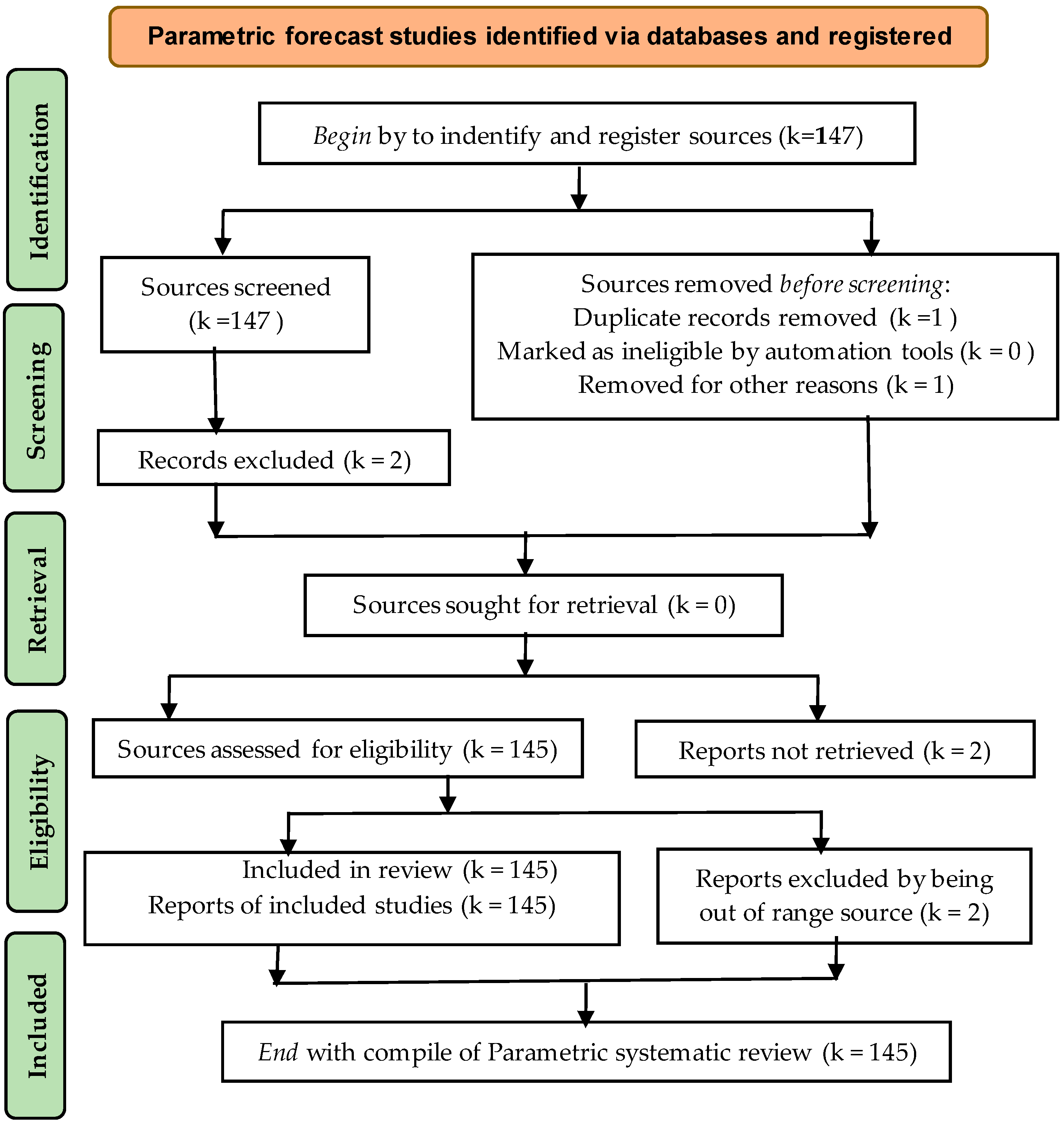

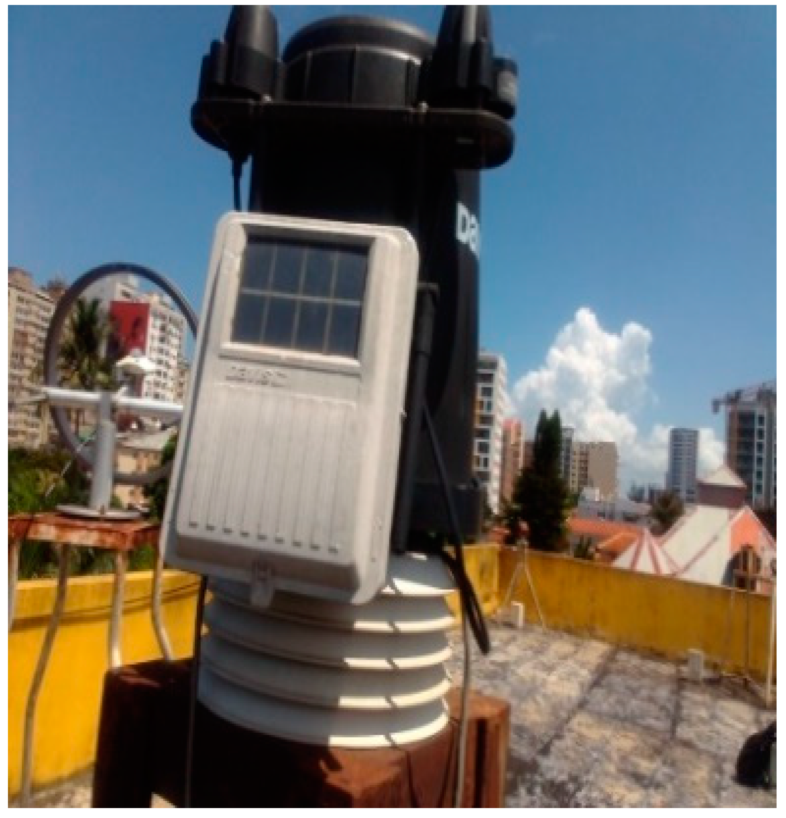
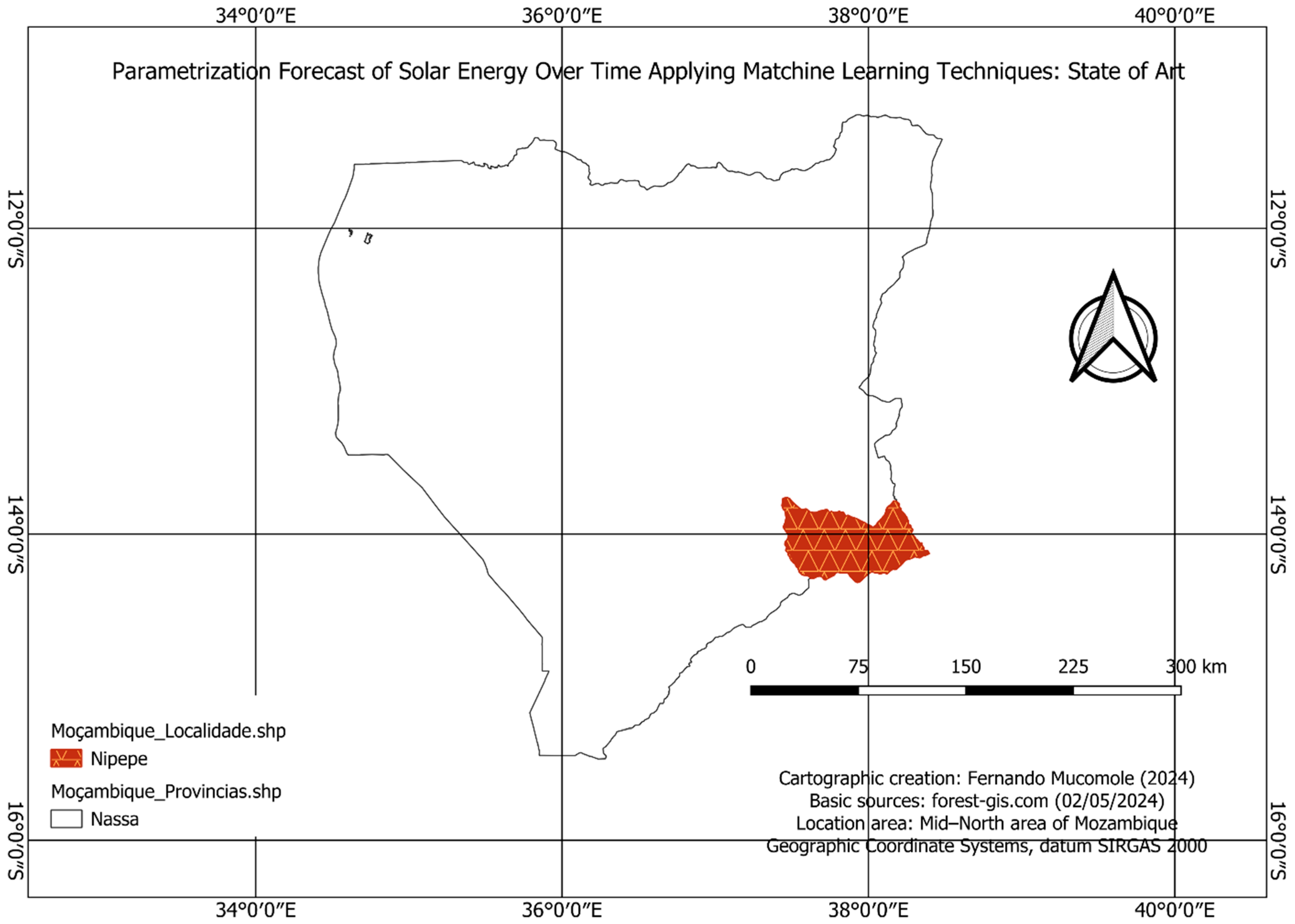
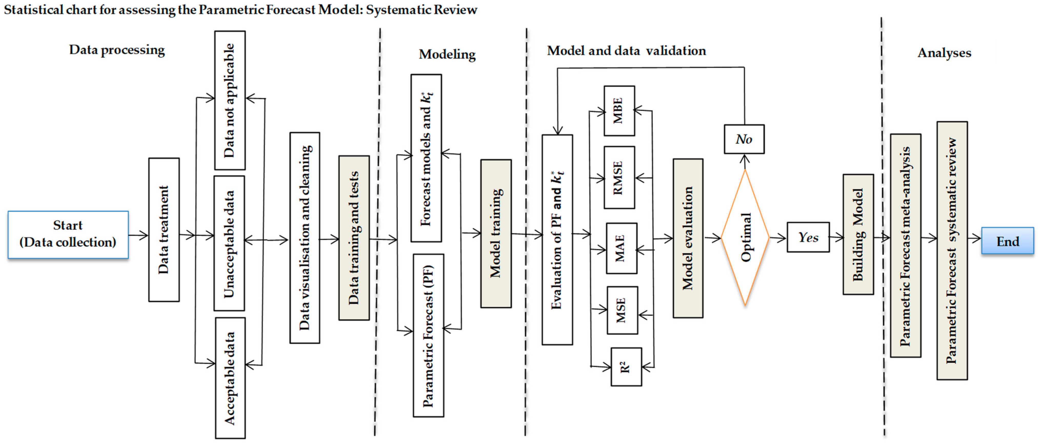
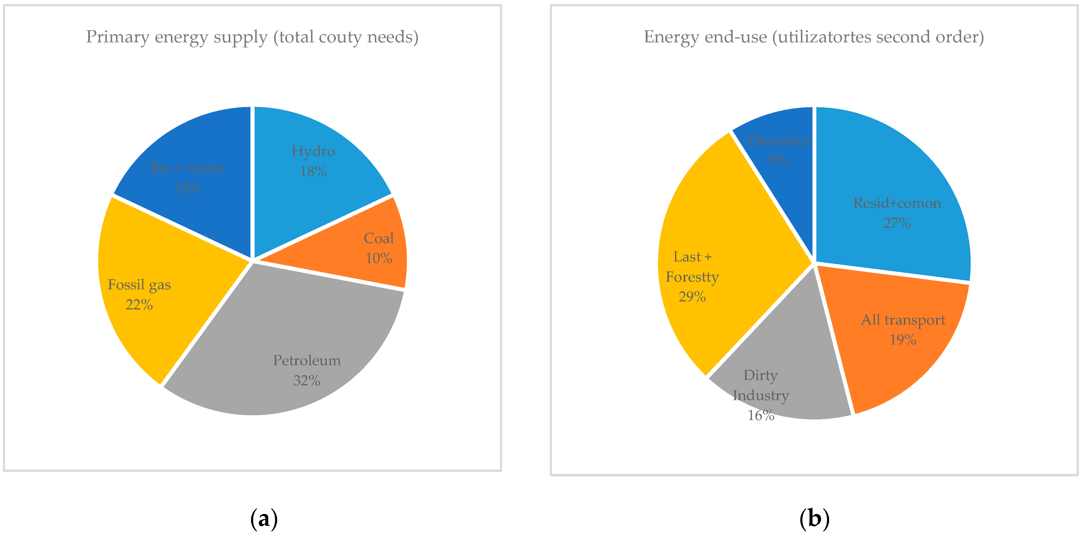
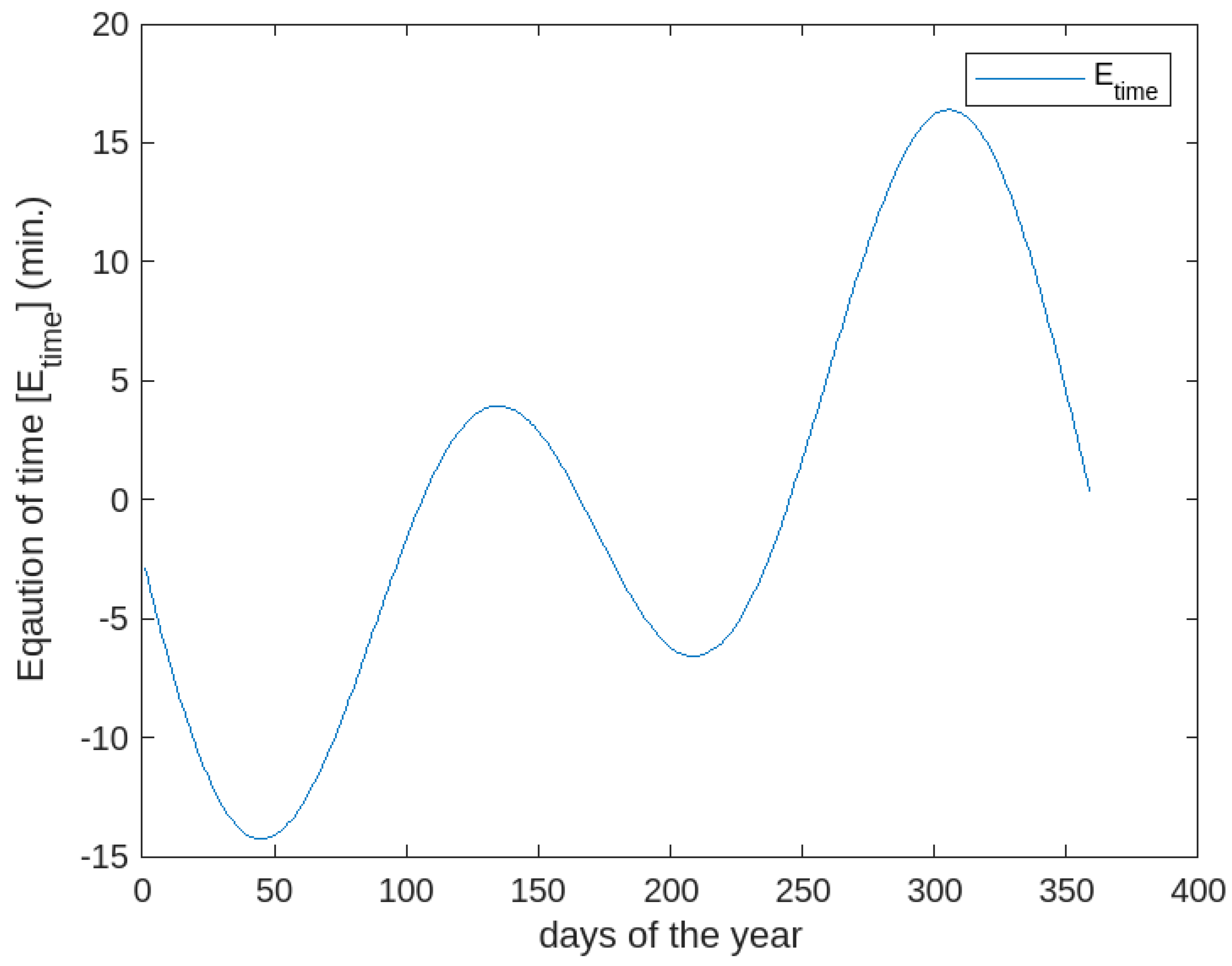
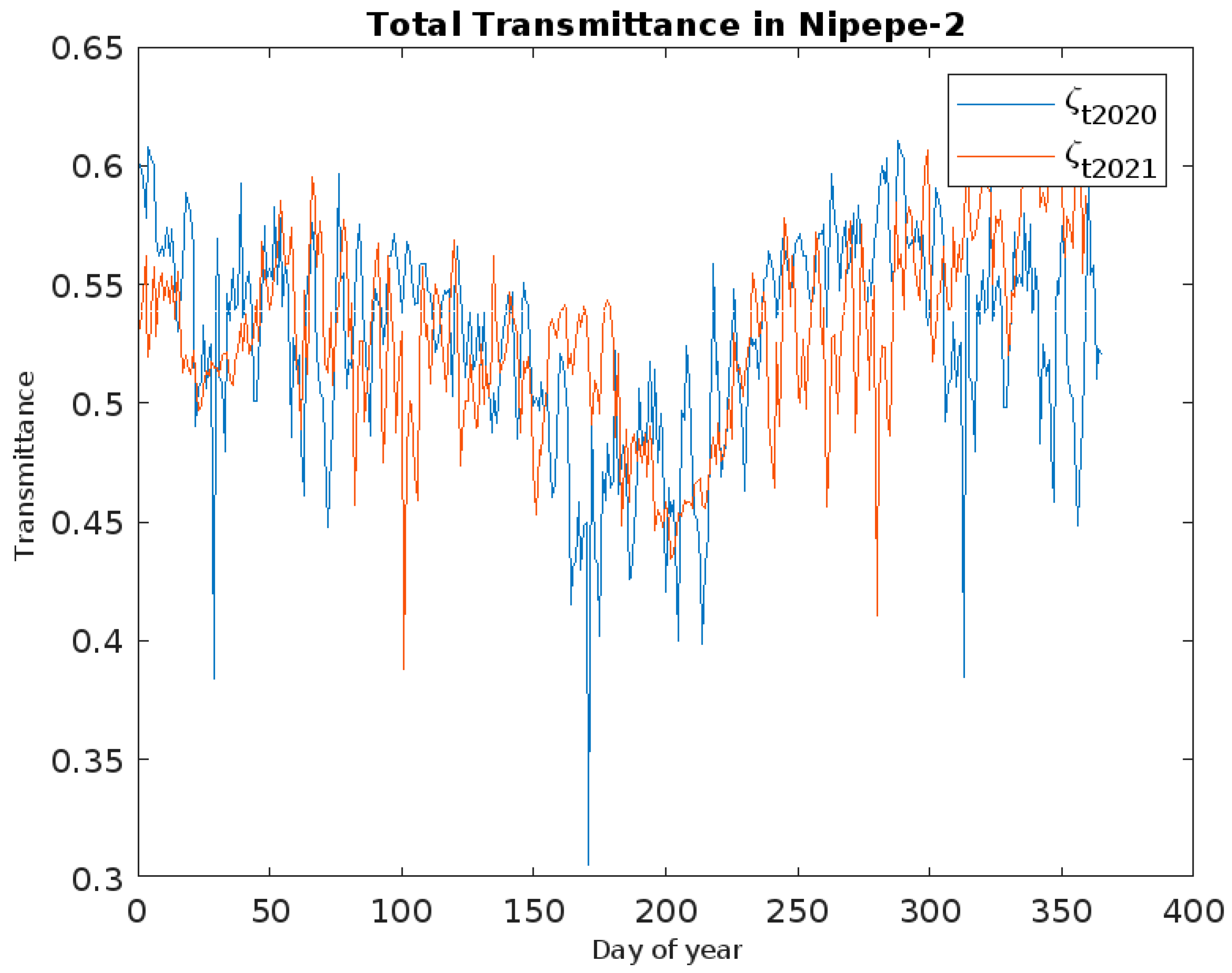
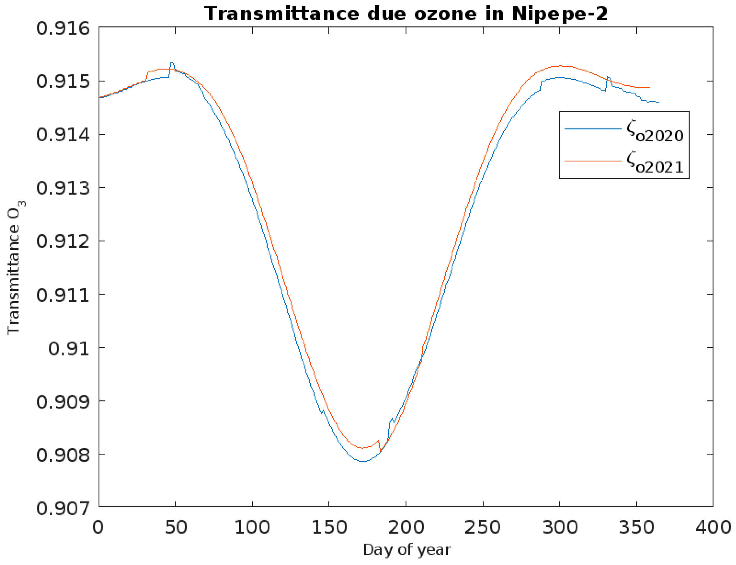
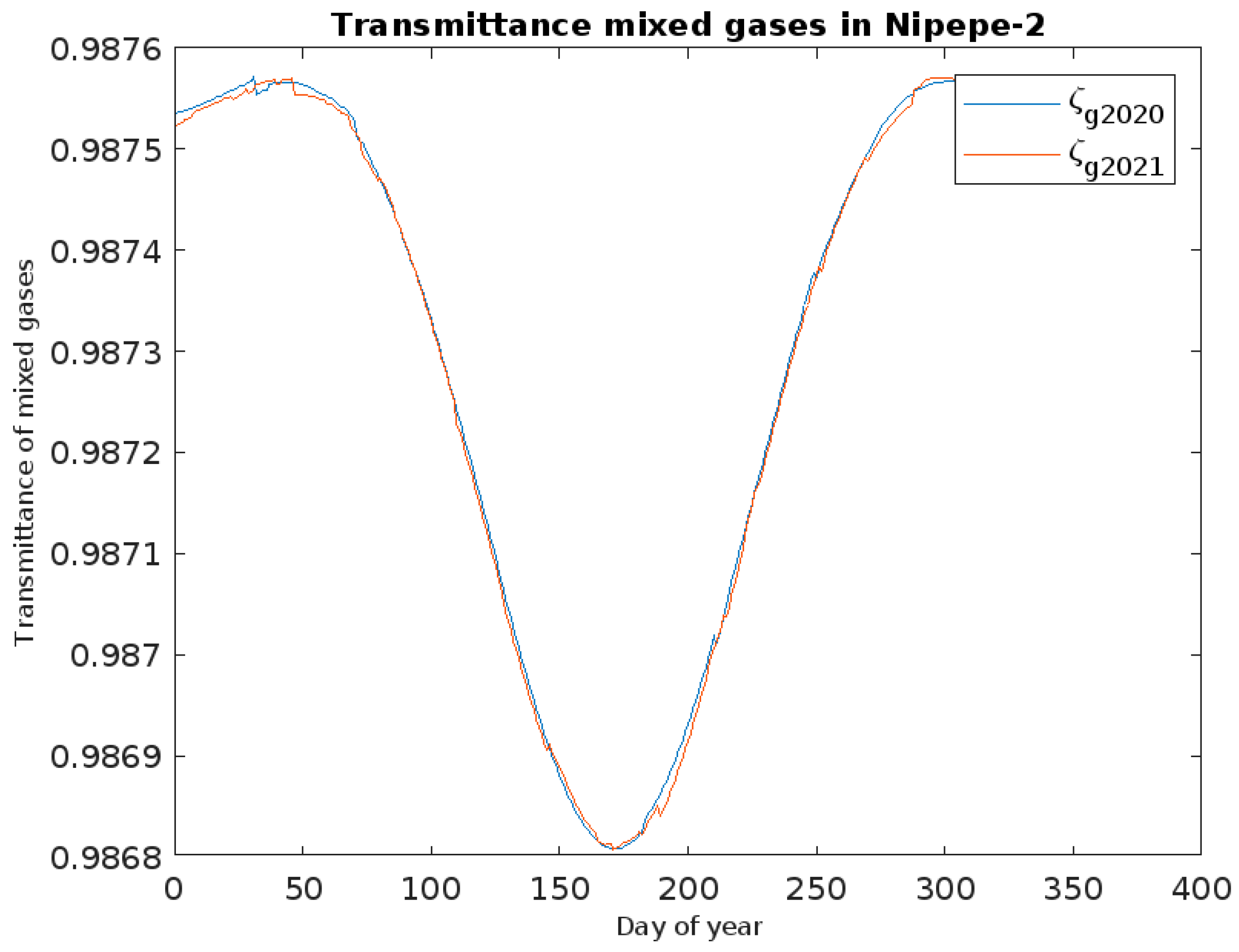
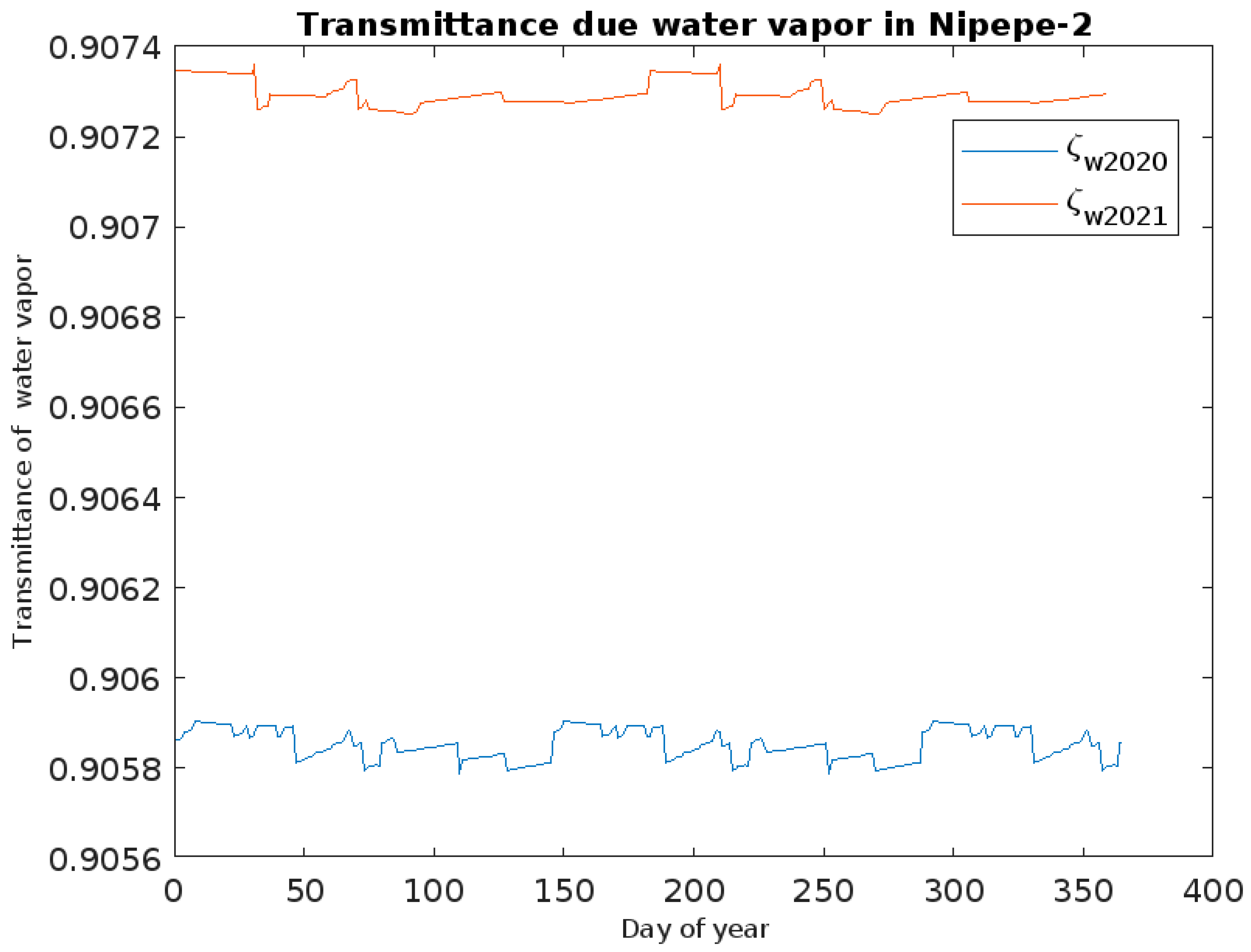
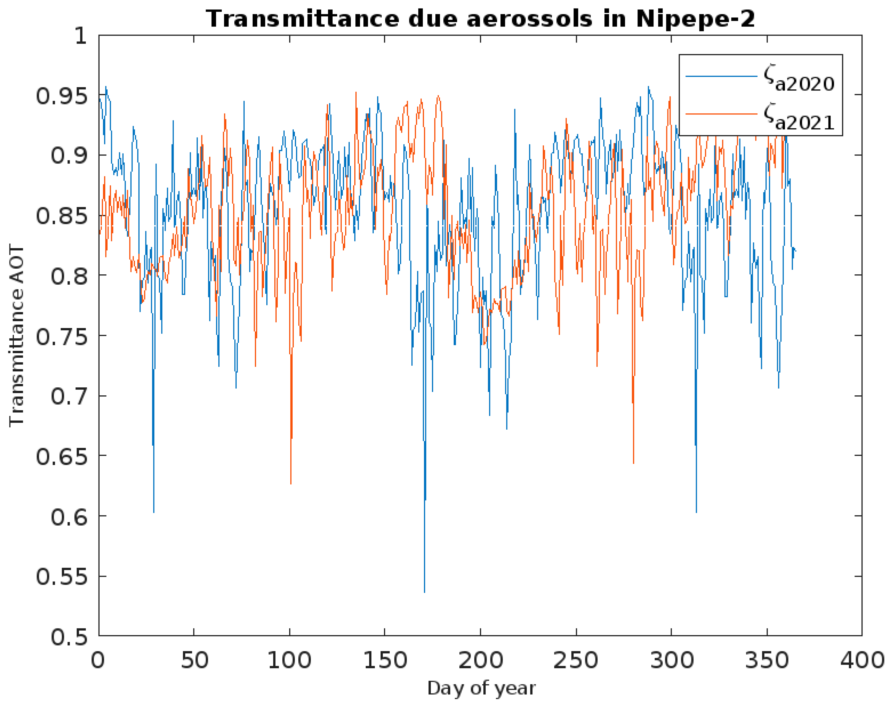
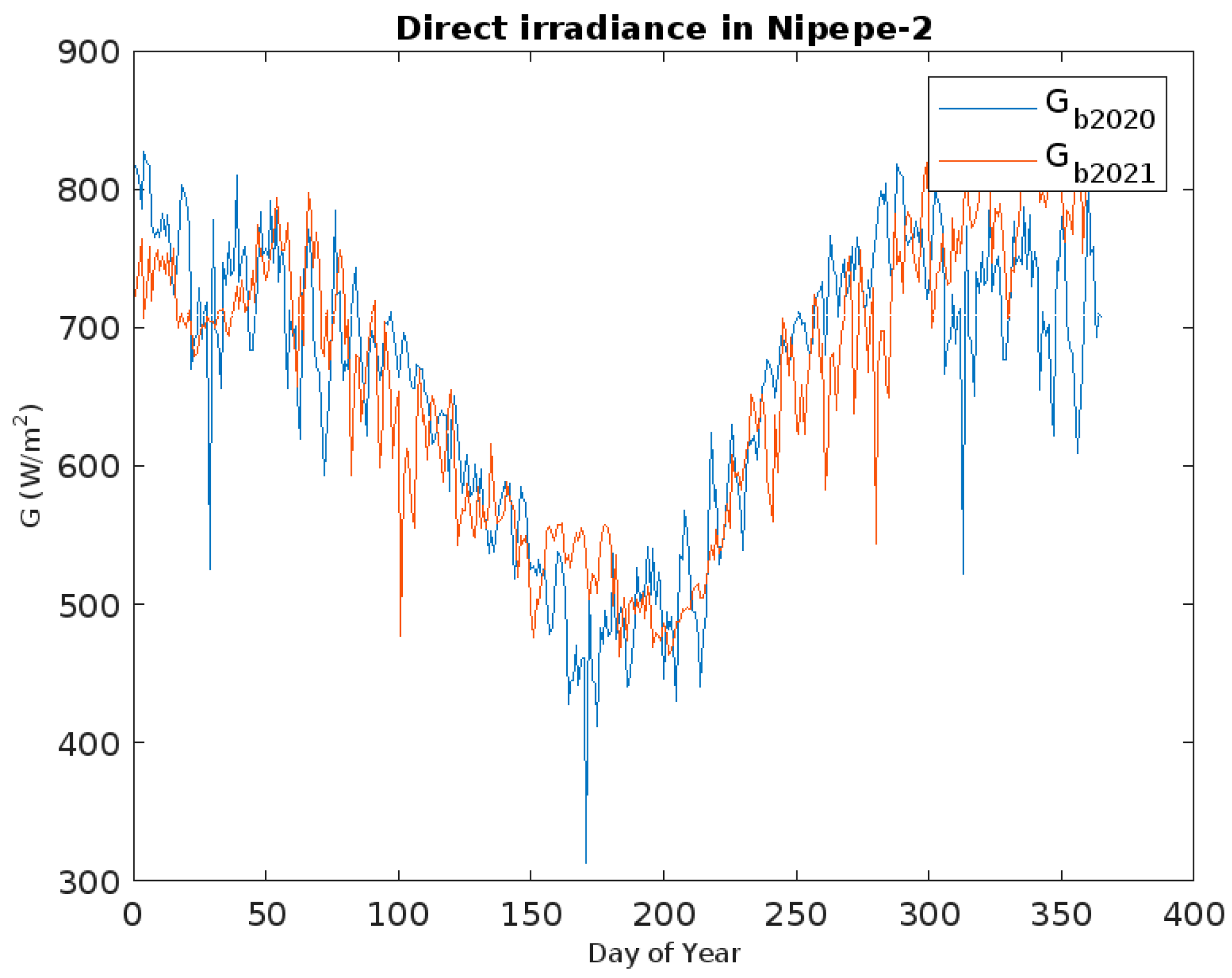
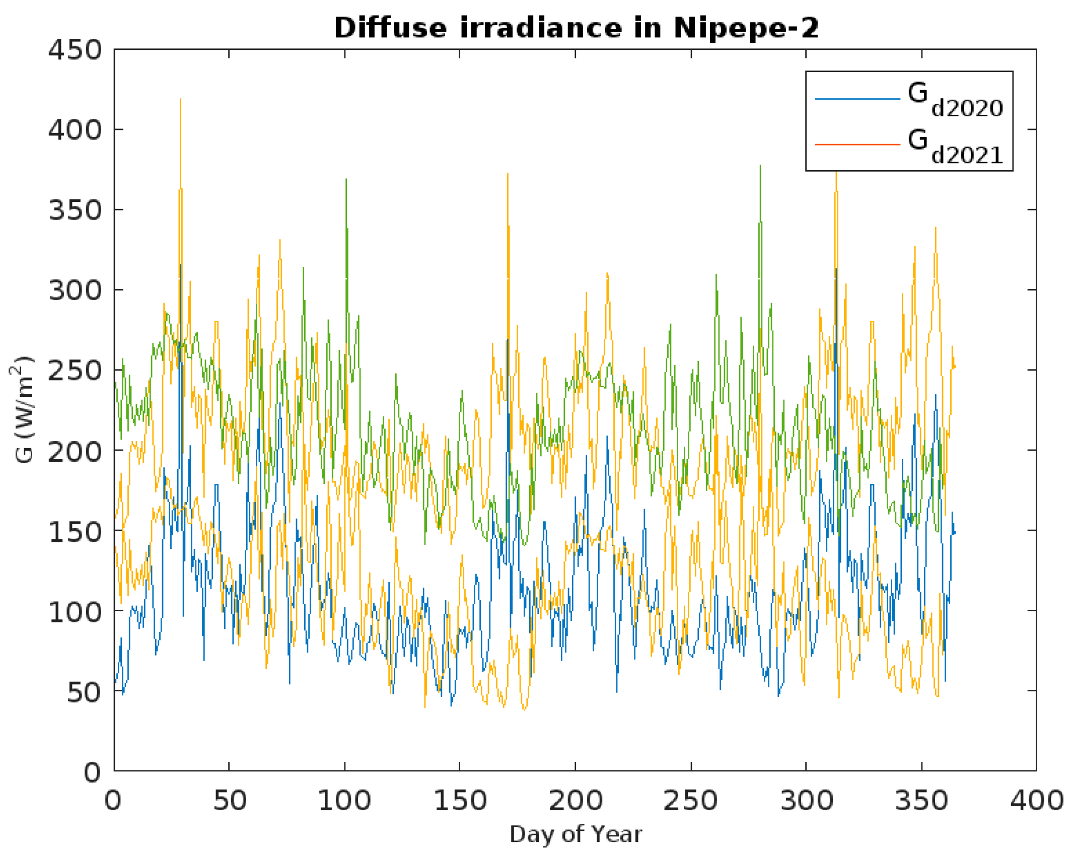
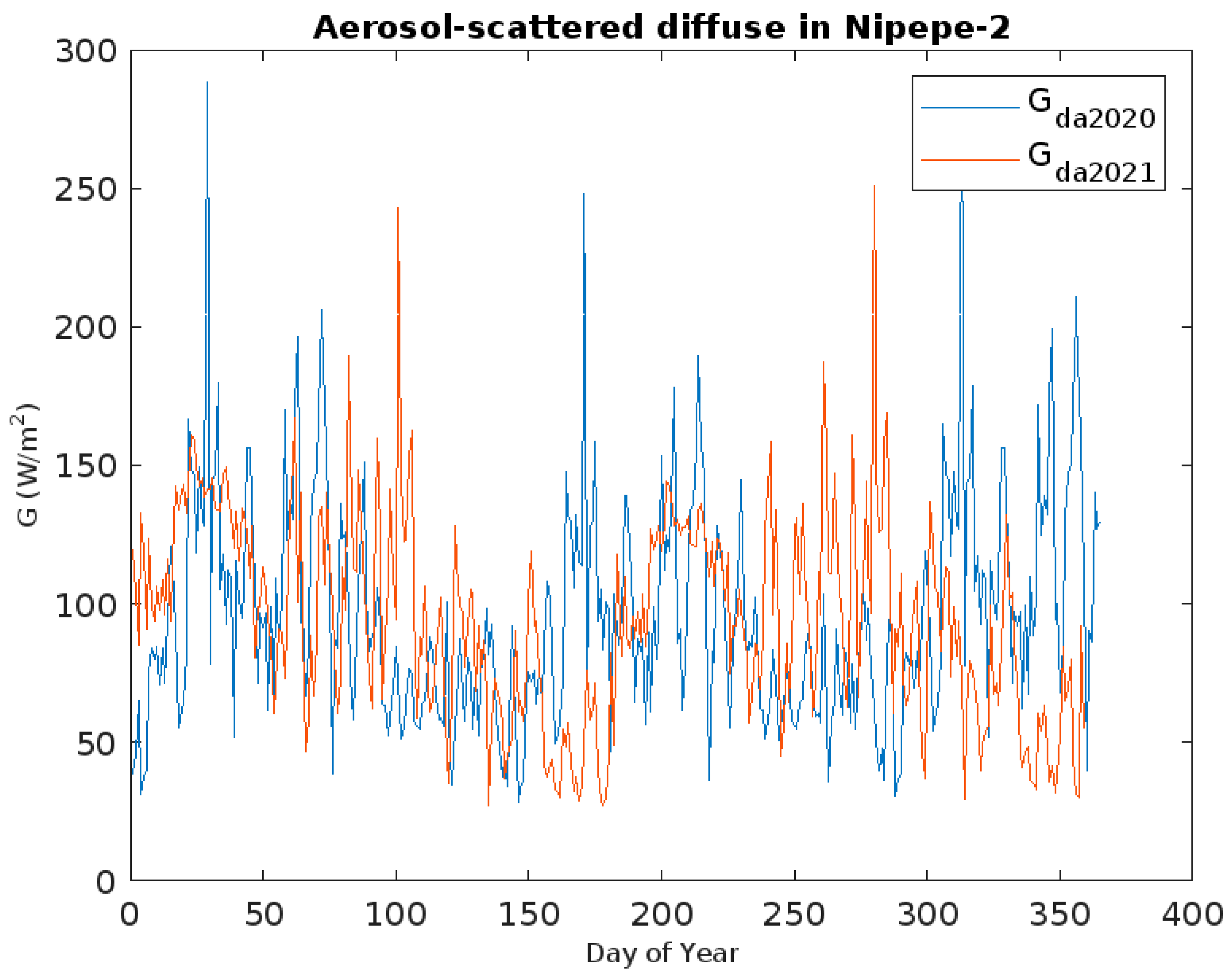
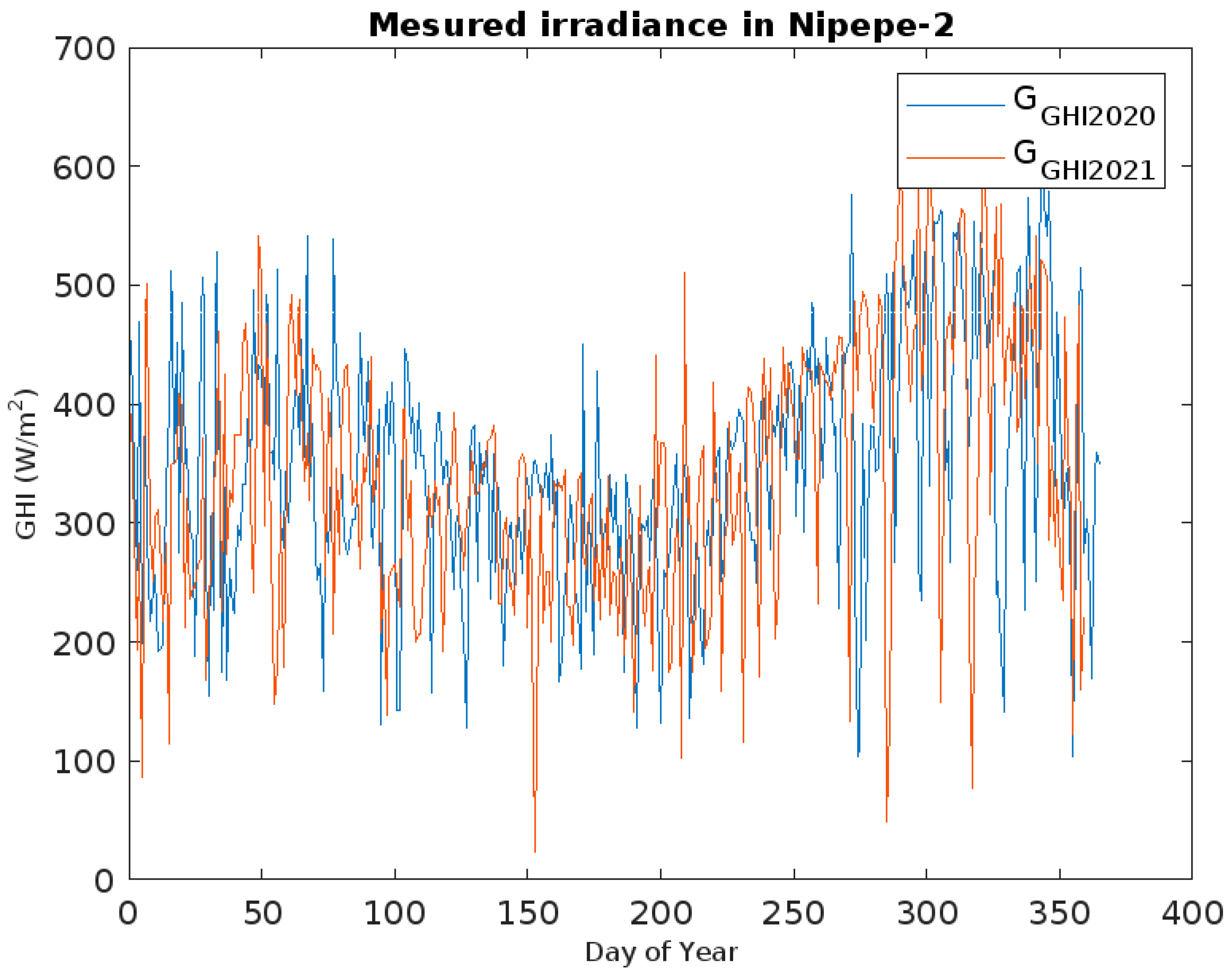
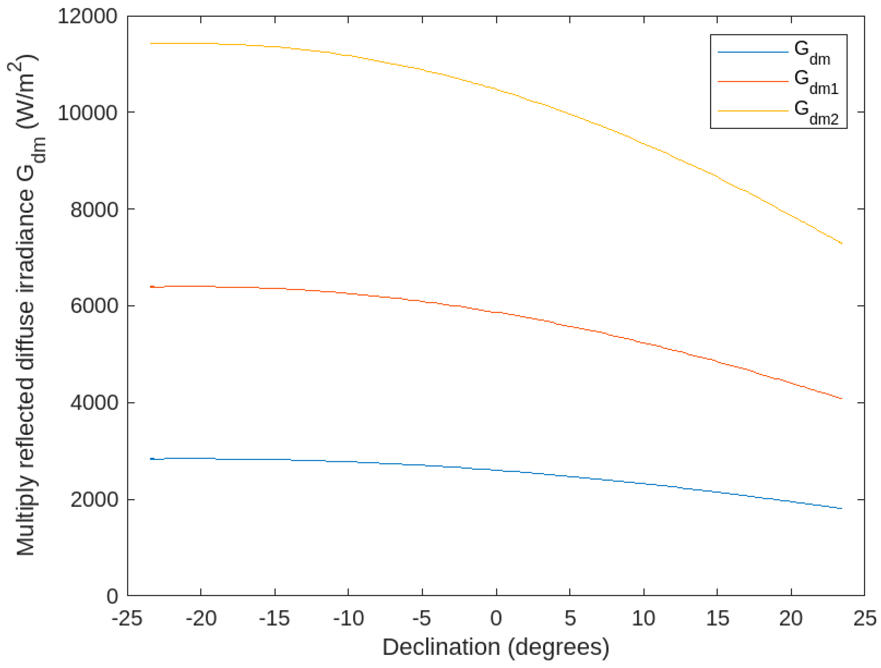
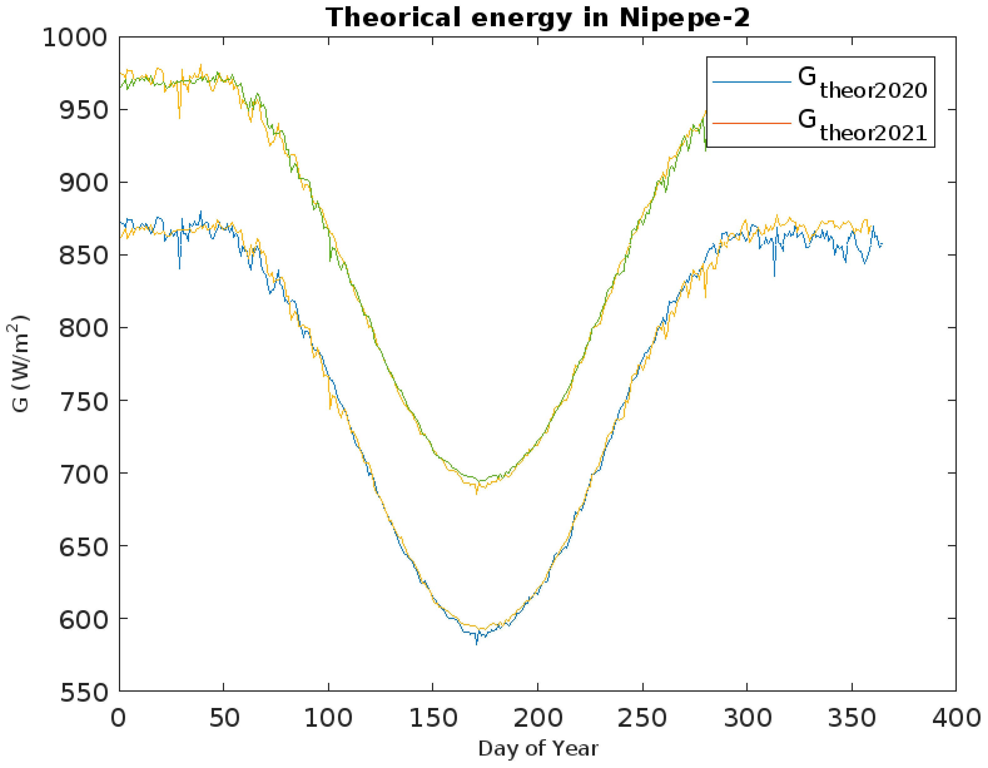
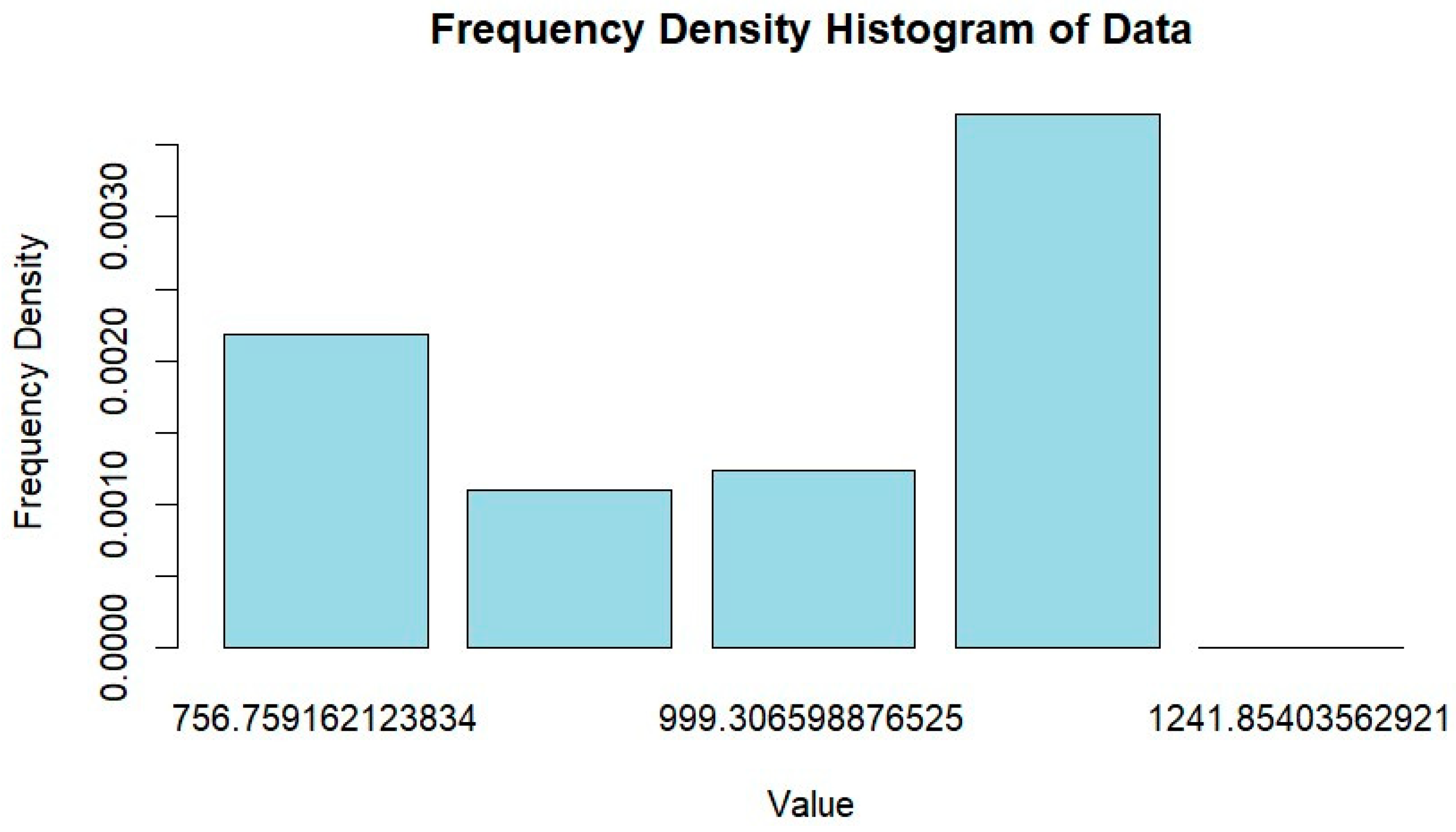
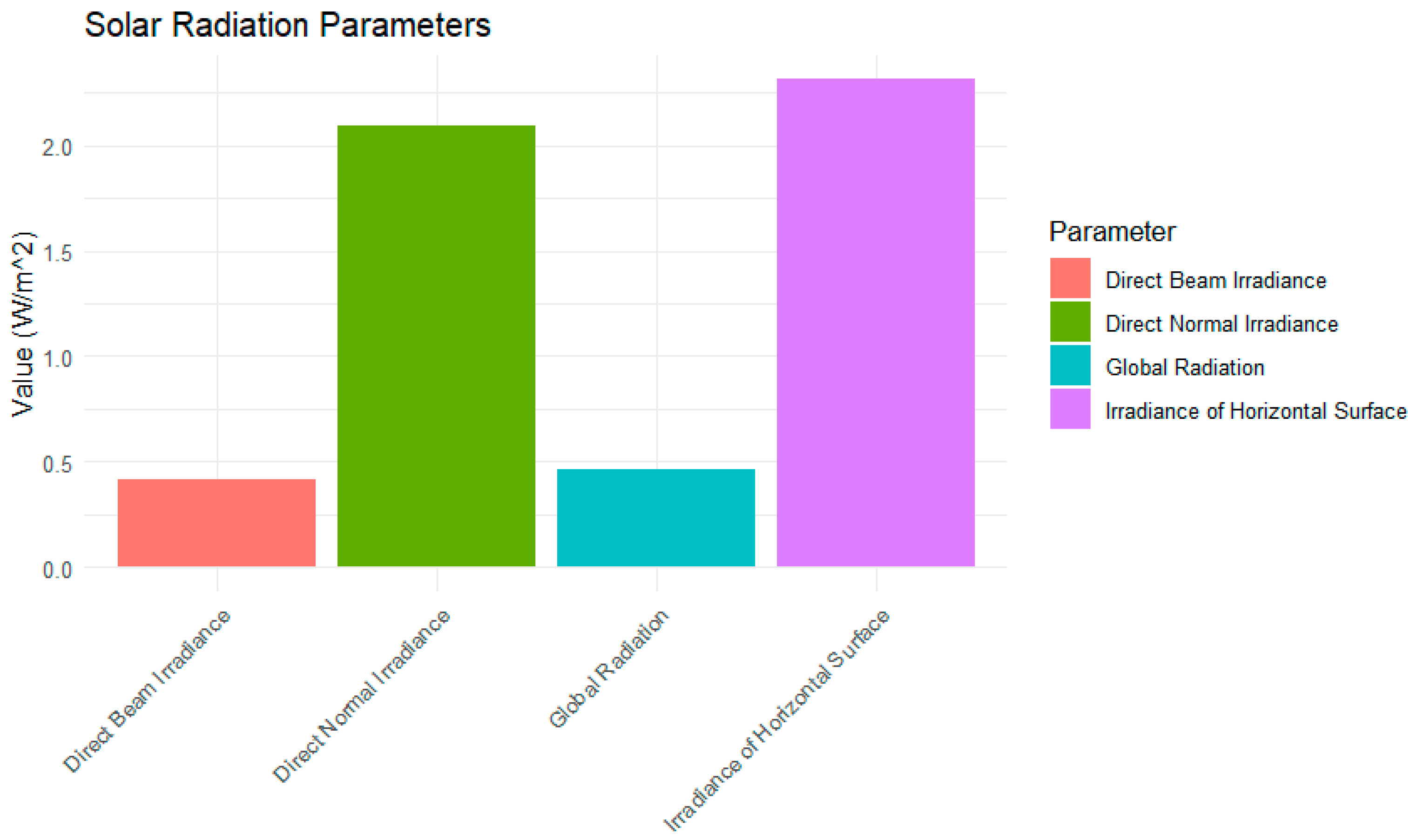
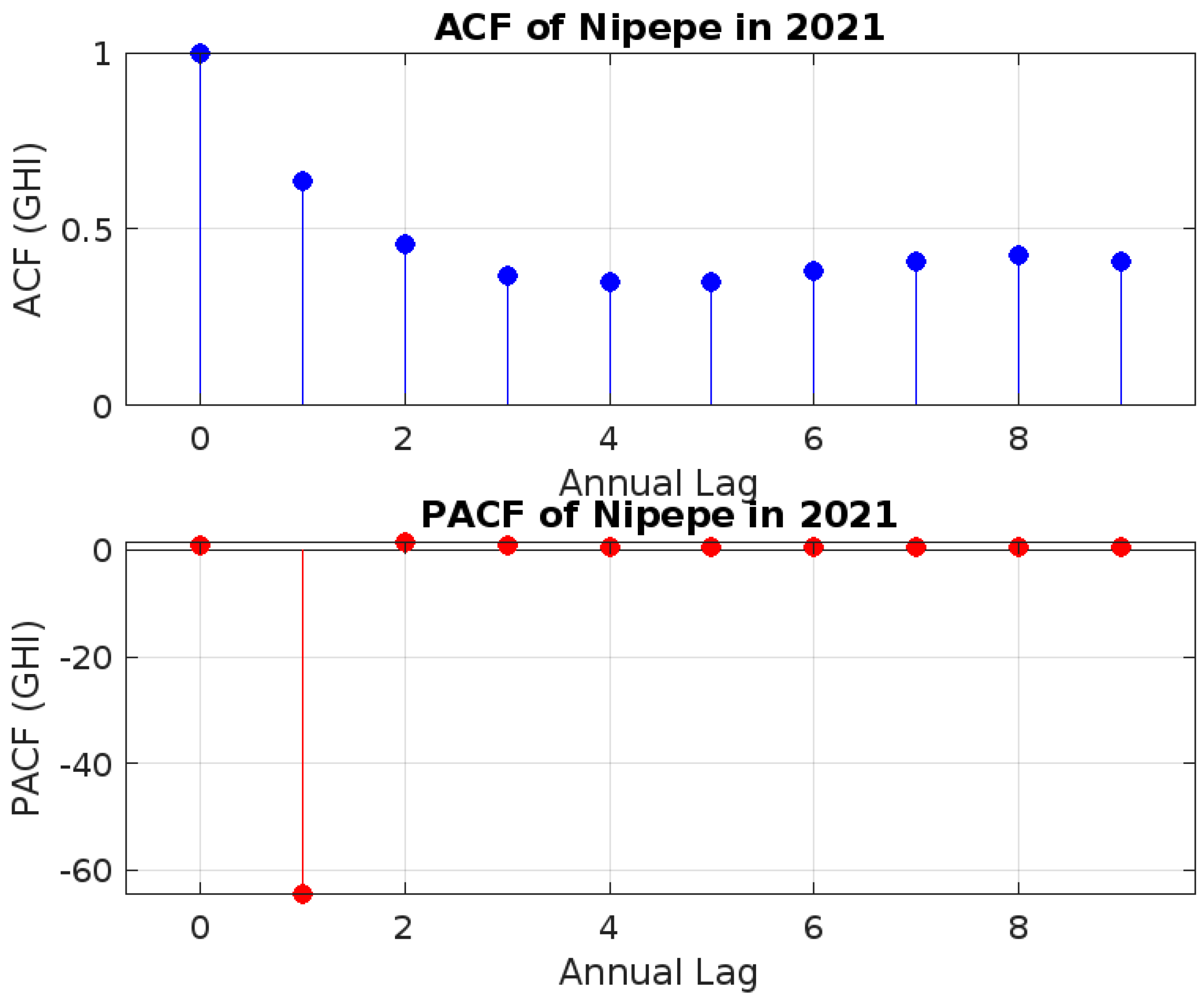
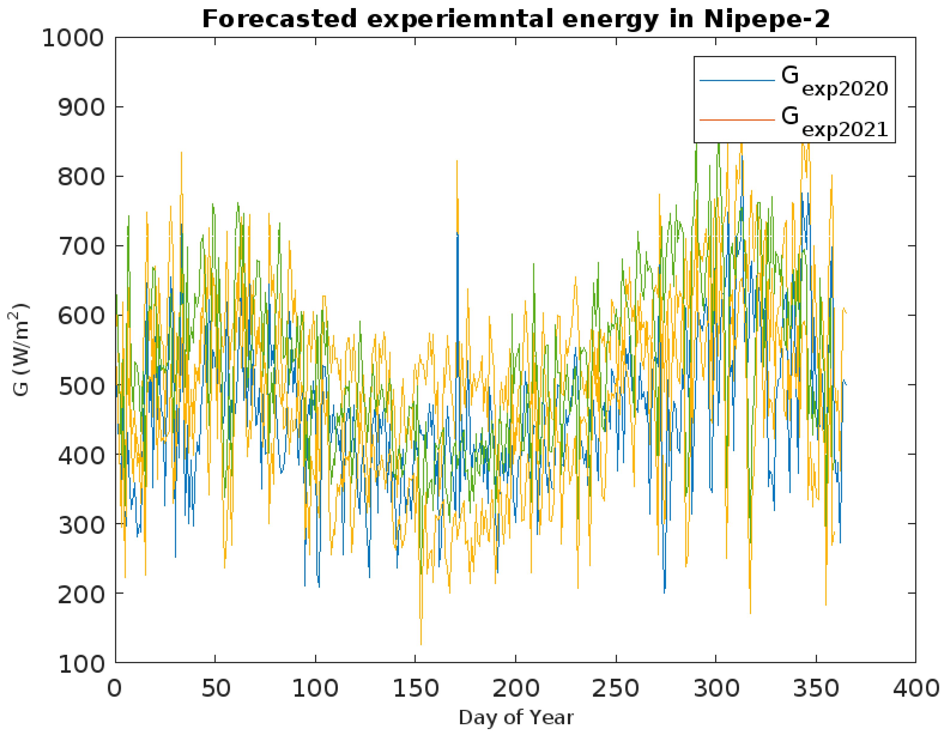
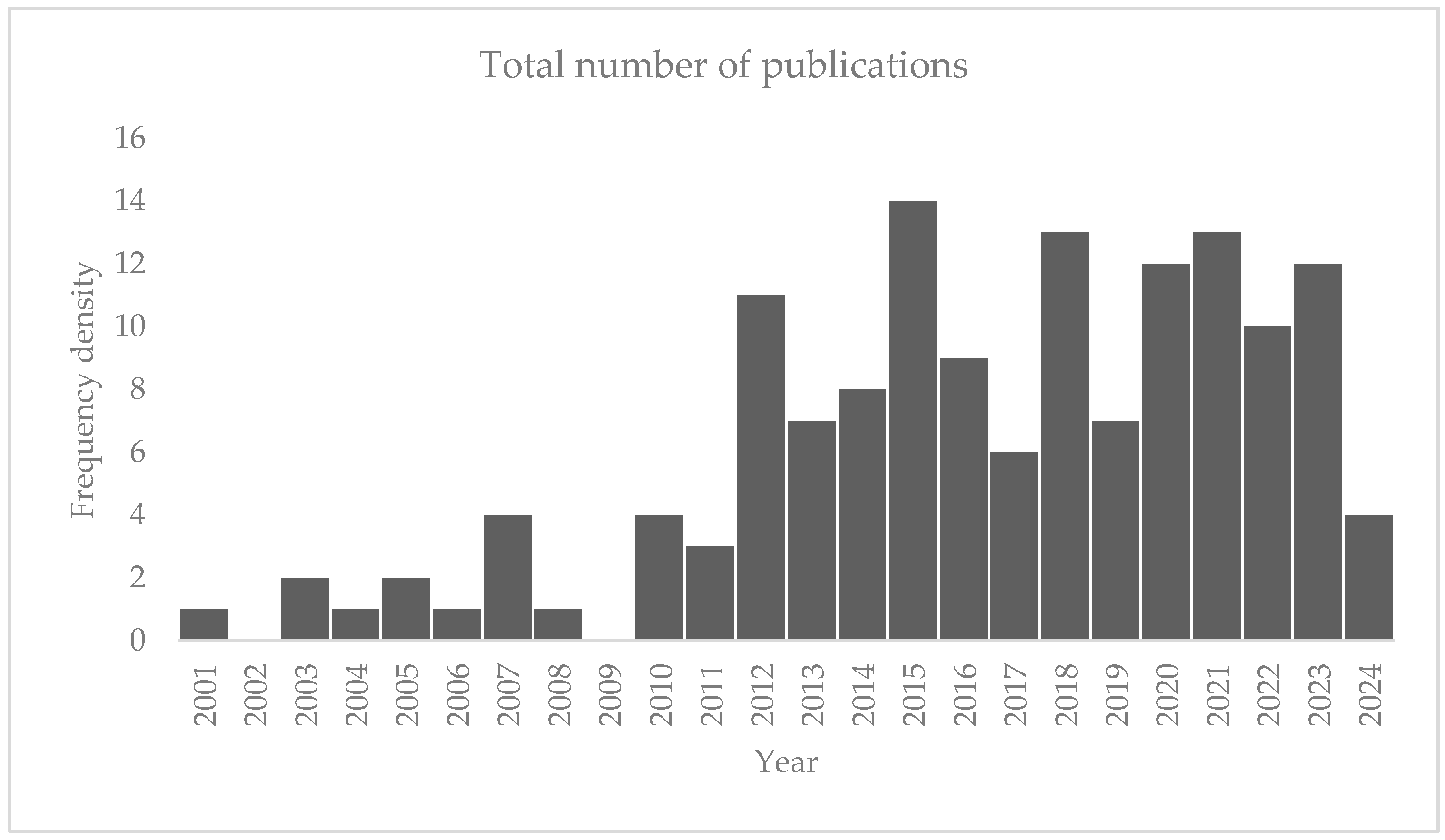


Disclaimer/Publisher’s Note: The statements, opinions and data contained in all publications are solely those of the individual author(s) and contributor(s) and not of MDPI and/or the editor(s). MDPI and/or the editor(s) disclaim responsibility for any injury to people or property resulting from any ideas, methods, instructions or products referred to in the content. |
© 2025 by the authors. Licensee MDPI, Basel, Switzerland. This article is an open access article distributed under the terms and conditions of the Creative Commons Attribution (CC BY) license (https://creativecommons.org/licenses/by/4.0/).