Abstract
The growing investment in variable renewable energy sources is changing how electricity markets operate. In Europe, players rely on forecasts to participate in day-ahead markets closing between 12 and 37 h ahead of real-time operation. Usually, transmission system operators use a symmetrical procurement of up and down secondary power reserves based on the expected demand. This work uses machine learning techniques that dynamically compute it using the day-ahead programmed and expected dispatches of variable renewable energy sources, demand, and other technologies. Specifically, the methodology incorporates neural networks, such as Long Short-Term Memory (LSTM) or Convolutional neural network (CNN) models, to improve forecasting accuracy by capturing temporal dependencies and nonlinear patterns in the data. This study uses operational open data from the Spanish operator from 2014 to 2023 for training. Benchmark and test data are from the year 2024. Different machine learning architectures have been tested, but a Fully Connected Neural Network (FCNN) has the best results. The proposed methodology improves the usage of the up and down secondary reserved power by almost 22% and 11%, respectively.
1. Introduction
The European Union’s energy and climate goals for 2030 and 2050 emphasize the transition to a carbon-neutral energy system, driven by the large-scale integration of variable Renewable Energy Systems (vRES), such as wind and solar photovoltaic (PV) technologies [1,2,3,4]. While vRES are critical for achieving sustainability targets, such as Sustainable Development Goals (SDG) 7 (Affordable and Clean Energy) and SDG 13 (Climate Action), their stochastic and intermittent nature poses significant challenges to power system operations, particularly in balancing energy supply and demand efficiently [5,6,7].
The increasing penetration of vRES introduces greater uncertainty into energy markets [8,9], particularly in Day-Ahead (DA) forecasts, which are essential for the allocation of the automatic Frequency Restoration Reserve (aFRR), also known as secondary reserves [10,11,12]. They are critical to guarantee the stable operation of power systems by maintaining frequency oscillations between technical constraints. Fast response power plants with high ramping-down and ramping-up capability, as pumped-hydro storage, are the main providers of secondary reserves [13,14]. These reserves, procured to address real-time imbalances between generation and consumption, often suffer from inefficient allocation methodologies. DA predictions frequently diverge from real-time conditions, leading to both over-allocation and under-allocation of reserves. This inefficiency not only results in higher operational costs but also compromises the optimal utilization of resources, thereby undermining the economic and energy efficiency of the system [15,16].
This paper focuses on enhancing the accuracy of DA forecasts for secondary reserve allocation, addressing the inefficiencies caused by vRES uncertainty [7,14,17]. By leveraging machine learning techniques, this work develops predictive models that incorporate historical data on vRES generation, demand patterns, and system behavior [18,19]. The objective is to dynamically adjust reserve allocations, ensuring that grid stability is maintained while minimizing excess reserve procurement [15,20]. Against this background, different machine learning architectures have been tested, mainly from the families commonly used in forecast modulation, such as convolutions, CNN; recurrent models, LSTM; and feed-forward models, FCNN. A deep, stacked, feed-forward architecture has the best results.
The work presented in this paper analyzes the benefits of using machine learning techniques for an independent, up and down, dynamic capacity procurement of secondary reserves. Publicly available operational data from the Spanish Transmission System Operators (TSO) were utilized, ensuring the replicability of the analysis. Typically, TSOs rely on bilateral agreements to acquire additional reserves, which can drive up costs. Analyzing the under-utilization of secondary reserves and the frequent need for extraordinary reserves in Spain highlights the inefficiencies in current methods for determining reserve requirements.
The Spanish TSO uses a deterministic approach to compute the size of the secondary reserve capacity. It was proved to be economical and technically inefficient. It only used an average capacity of around 25% of the total allocated capacity, which resulted in four times more expenses than needed. Even considering such a conservative approach, the average annual missing energy stands at around 1% of the total allocated capacity [13,15,16,20]. Therefore, during those events, the TSO has to contract an extraordinary secondary reserve capacity to guarantee the frequency stability and security of supply. Therefore, while the potential of a perfect foresight solution is an improvement of 75%, the best methodology (FCNN) tested in this work improves the usage of the up and down secondary reserved power by almost 22% and 11%, respectively.
The remainder of this paper is structured as follows: Section 2 presents a literature review on dynamic reserves and machine learning. Section 3 provides an overview of wholesale energy markets and reserve systems, highlighting existing inefficiencies. Section 4 outlines the proposed methodology for dynamic reserve allocation using machine learning techniques. Section 5 presents a case study and evaluates the performance of the developed models. Finally, Section 6 summarizes the findings and discusses the implications for future energy systems.
2. Literature Review
The increasing integration of vRES in power systems has created significant challenges for electricity markets and ancillary services. Traditionally, TSOs rely on the symmetrical allocation of upward and downward reserves based on deterministic forecasts of demand. However, with vRES like wind and solar introducing substantial variability and unpredictability, these conventional methods have proven inefficient in addressing the real-time balancing needs of modern power systems [5,6,7].
The European Network of Transmission System Operators for Electricity (ENTSO-E) framework [21] outlines standardized methodologies for reserve sizing, which are Frequency Containment Reserve (FCR), aFRR, and manual Frequency Restoration Reserve (mFRR), which often fail to adapt dynamically to changing system conditions. In Portugal, for example, the secondary reserve allocation formula used by the TSO employs a fixed ratio applied to expected demand, resulting in excessive allocation [3,16]. Similar inefficiencies are observed in the Spanish procurement of secondary (aFRR) reserve capacity, where it lacks adaptability to vRES production and correlation with real-time balancing needs [15,22]. Indeed, after the European gas crisis, the Spanish TSO changed the allocation of reserve capacity in the middle of 2022 to a more conservative, practically symmetrical procurement [22,23]. The procurement of secondary capacity increased to a similar level across the day and is typical of peak procurement. The procurement of down capacity significantly increased to values close to up capacity. Since the middle of 2022, the procurement of secondary capacity has been less dynamic and volatile throughout the day, decreasing the usage percentage of secondary capacity [15,22].
Numerous studies highlight the limitations of static reserve procurement methods under high vRES penetration. The majority of the literature focuses on using historical data to compute the procurement of secondary reserves [17,24,25]. Operational methodologies are needed to be used by TSOs. Dynamic procurement of secondary reserves has been proposed to address these inefficiencies, with an improvement of 13% and 8% for up and down secondary capacities by 2022 [20]. By incorporating real-time or near real-time forecasts of demand and renewable generation, dynamic methodologies aim to optimize reserve allocation, reducing operational costs and resource wastage. Furthermore, five different mechanisms for procuring secondary power in Spain were analyzed for the Spanish power system by 2030, with renewable penetrations higher than 70% [15]. The dynamic procurement methodology proposed in this study enables cost reductions for Spanish secondary power by 27% when using block bids and 34% when using flexible bids. These results highlight the increasing importance of dynamic reserve procurements with the rising uncertainty of higher penetrations of vRES.
Machine learning techniques have emerged as a powerful tool to support this transition. Studies such as [18,19] demonstrate the potential of predictive models to estimate reserve needs with greater accuracy, leading to significant reductions in over-procurement. De Vos et al. proposed a machine learning approach to estimate imbalance uncertainty, to adjust the size of Belgium’s operating reserves from an annual to a daily basis, resulting in a 5% reduction [18].
Kruse, Schäfer, and Witthaut introduced an ex post machine learning method to determine the appropriate size for secondary reserves. They identified key variables that most accurately estimate errors, essential for detecting when secondary control is activated. Additionally, to enhance the efficiency of cross-border capacity allocation in balancing service exchanges, legislation recommended coupling balancing mechanisms, as demonstrated in the Nord Pool market [16,26].
Cardo-Miota et al. identified the benefit of using machine learning techniques to predict the prices of aFRR in Spain [22]. The literature also underscores the importance of enhancing forecast accuracy for vRES generation and consumption patterns. Traditional statistical models, including ARMA and ARIMA, have been widely used for time series forecasting. However, recent advancements in machine learning, such as LSTM networks and CNN, have shown superior performance in capturing the nonlinear and temporal characteristics of renewable energy data [27,28]. These models can adapt to complex patterns and improve prediction accuracy, enabling more efficient management of reserves.
Therefore, most studies use machine learning techniques to improve the market outcomes of their participants. Moreover, on the subject of the presented article, most studies use historical data analysis to define the size of the secondary capacity. This study presents an operational open-source methodology that can be tested and adapted by TSOs. Against this background, while the literature presents rich forecasting approaches to accurately predict vRES production using machine learning techniques, TSOs still use deterministic conservative methodologies to procure secondary capacity. Indeed, vRES and demand-side players are the main sources of real-time deviations, and forecast methodologies are being improved to reduce the penalties they pay for imbalances. Therefore, TSOs will also consider the stochastic nature of those imbalances while predicting the secondary energy needs.
In summary, the following three key areas of focus has been identified in the literature: the inefficiency of static reserve allocation methods, the potential of machine learning to improve forecasting accuracy, and the need for market design adaptations to support dynamic reserve procurement. This paper builds upon these insights by applying machine learning techniques to optimize secondary reserve allocation, addressing forecast uncertainty and market inefficiencies.
3. Electricity Markets and Ancillary Services
The operation of modern electricity systems relies heavily on well-structured markets to ensure the balance between generation and consumption. These markets encompass wholesale electricity markets, where energy is traded, and ancillary services markets, which guarantee the system’s stability and reliability. The integration of vRES has added complexity to these operations, requiring more dynamic approaches to market design and reserve allocation.
3.1. Wholesale Electricity Markets
Wholesale electricity markets facilitate the trading of electricity between generators, suppliers, and other market participants [29]. These markets are typically divided into three main categories: day-ahead markets (DAM), intraday markets (IDM), and real-time balancing markets [8]. In the DAM, participants submit bids for energy delivery 12 to 37 h before real-time operation. The market-clearing process determines the energy schedules and market prices based on supply and demand equilibrium [9]. While the DAM provides a foundation for energy trading, the IDM allows participants to make adjustments closer to real time, responding to unforeseen changes in demand or vRES generation.
Balancing markets, on the other hand, operate in near real time to address deviations between scheduled and actual energy delivery. TSOs procure balancing services to ensure system equilibrium, activating reserves as needed. This process is particularly critical in systems with high vRES penetration, where forecasting errors can cause significant imbalances [12,14].
3.2. Ancillary Services and Reserve Requirements
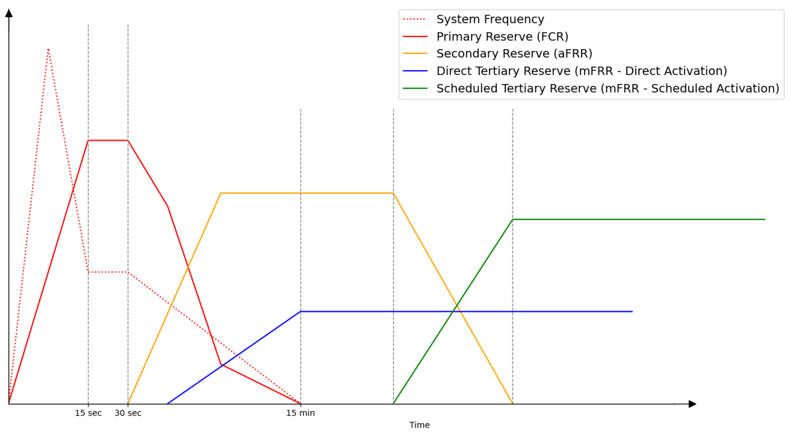
Ancillary services are essential for maintaining grid stability and ensuring a reliable power supply. They include services such as frequency control, voltage regulation, and operating reserves. Among these, frequency control reserves play a crucial role in balancing supply and demand in real time. These reserves are divided into the following three main categories [14] as presented in Figure 1:
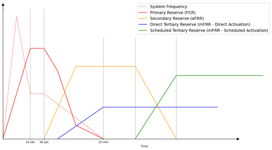
Figure 1.
Ancillary services response scheme. Adapted from [21].
- FCR: Activated automatically within seconds to stabilize frequency deviations;
- aFRR: Restore frequency to nominal levels and release FCR for subsequent use;
- mFRR: Address longer-term imbalances through manual activation.
3.3. Iberian Reserve Markets
The Iberian Market of Electricity (MIBEL) is an example of energy market integration across countries. It acts as a bond between Portuguese and Spanish electricity markets, Operador do Mercado Ibérico de Energia Português, Sociedade Gestora do Mercado Regulamentado, S.A. (OMIP) and Operador del Mercado Ibérico de Energía—Pólo Espanhol, S.A (OMIE). This joint market consists of bilateral, derivative, and spot markets. Even though there is a joint market, each country’s TSO, Red Eléctrica de España (REE) for Spain and Redes Energéticas Nacionais (REN) for Portugal, manages its own ancillary services independently.
Static Reserve Procurement
In Europe, the ENTSO-E provides guidelines for the procurement and activation of these reserves. Traditionally, TSOs acquire reserves symmetrically (equal upward and downward capacities) based on deterministic demand forecasts. However, this approach often leads to inefficiencies in systems with high vRES variability. For secondary reserve, the ENTSO-E proposes
where
- R: secondary control reserve;
- a and b: empiric coefficients, a = 10 MW and b = 150 MW;
- : maximum anticipated consumer load.
The Spanish and Portuguese markets provide examples of differing reserve procurement methods. In Portugal, the TSO employs a fixed ratio formula for secondary reserve sizing. This creates a symmetrical distribution for upward and downward bands, respectively, and of the reserve band.
The given formula is based on ENTSO-E Equation (1), adding an hourly ratio , as follows:
The hourly ratio varies between 20% (1.2) and 60% (1.6), upscaling the the ENTSO-E suggestion for up regulation. Conversely, the Spanish market lacks a standardized reserve procurement formula, relying instead on a more flexible procurement mechanism [24], where the upward and downward bands’ distribution is not directly symmetrical. These differences highlight the need for market design improvements to better accommodate the variability of vRES.
4. Dynamic Procurement of Secondary Power
This study proposes a dynamic procurement based on machine learning techniques, trained with historical hourly data with custom-made model architectures.
4.1. Methodology Implementation
The methodology applied was a “brute force” choosing of a better model, which can lead to better fine-tuning results than a more complex architecture, as shown in [30].
Multiple model-related variables in this study are presented in Table 1.

Table 1.
Training and architecture variables.
This has been studied with different architectures and has already been proven to work in energy forecast [31] or in forecast in general [32], such as FCNN, LSTM, and CNN. Additionally, testing architectures has been proven to work in other fields, such as UNET [33] from image segmentation or Transformers [34], the current machine learning state-of-art architecture. However, with regard to Transformers, the processing limitation will not allow for a deep study of the potential on the given problem.
As regards the loss function used, it will be tested with the three most common regression loss functions, Mean Absolute Error (MAE), Mean Squared Error (MSE), and Mean Squared Logarithmic Error (MSLE), which are means of the given error, in absolute terms; the square of the errors; and the logarithmic square, respectively. The last two functions give more importance to larger errors.
However, since this problem is not only about finding the smallest error, but also about making sure that there are fewer negative and positive errors than the benchmark, a custom loss function has been created to encapsulate the final loss calculation, the Mirror Weights (https://github.com/alquimodelia/alquitable/blob/main/alquitable/advanced_losses.py#L33, accessed on 9 March 2025).
This function acts as a weight distributor for the negative and positive errors in such a way that the ratio defines which size gives more meaning to the final loss calculation. This was created since the error in missing energy is on a dimension and on surplus .
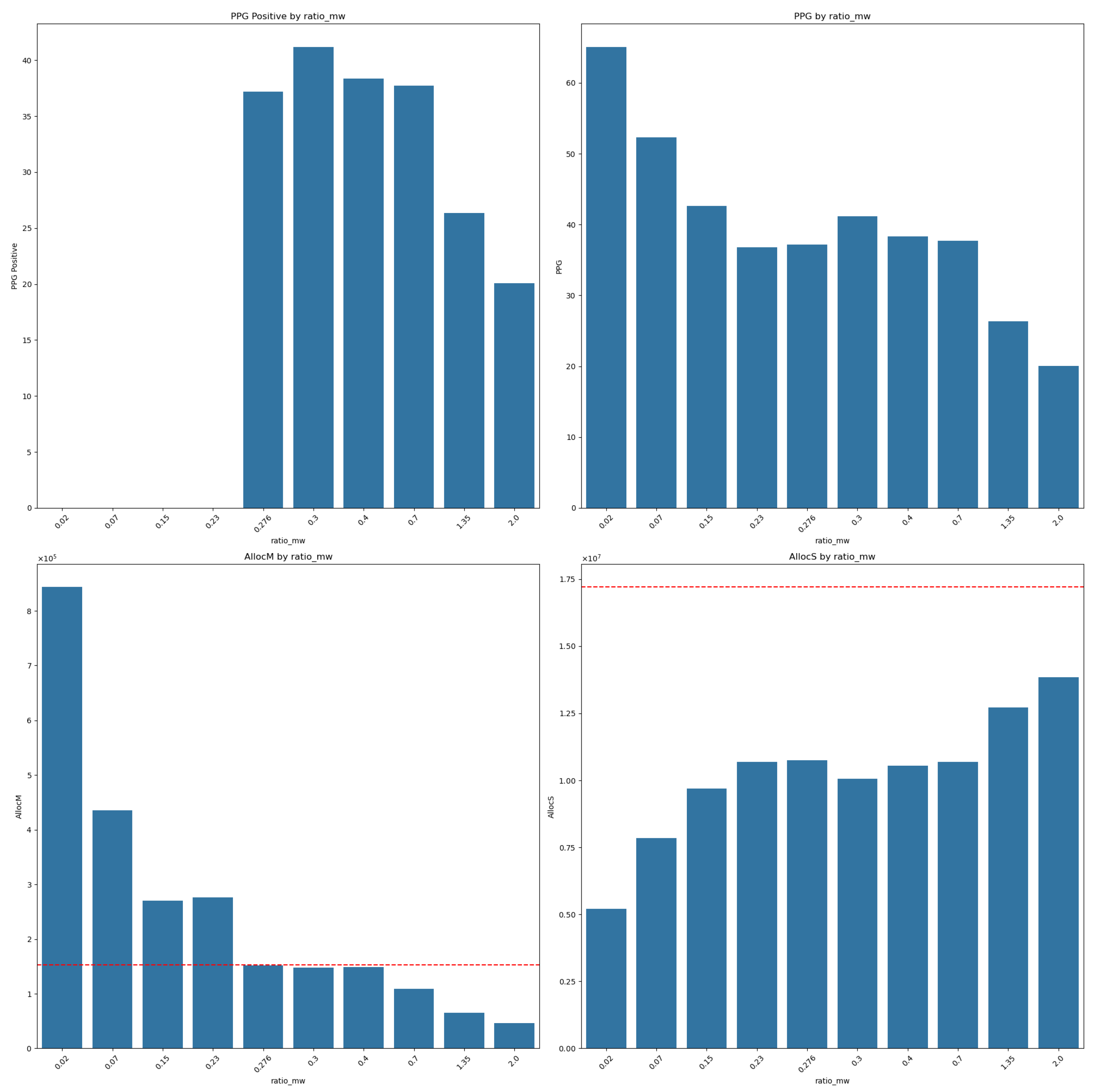
In a default loss function trying to lower the absolute error, this difference means most work would be to lower surplus errors even at the expense of raising the missing error. The created function allows for more behaviors, and some of them were studied, but the one with better results was defaulting surplus results weight 1 and making the weights of missing values its own error, multiplied by a ratio. Insights on given different ratio outcomes can be seen in Figure 2. In Figure 2, the red dotted line shows the benchmark values, and our goal is to have both below the benchmark line.

Figure 2.
Mirror weights ratio influence on metrics.
As regards the activation research suggested, it could have a significant impact on the outcome [30,34]. The test was conducted using the most common activations for regression problems, where we separated activations inside the model structure (on each deep layer) and the final layer. That is, the linear leaves inputs unchanged, the Rectified Linear Unit (ReLU) outputs the input if positive and zero otherwise, and the Gaussian Error Linear Unit (GELU) smooths this behavior by applying a Gaussian-based probabilistic transformation.
The last model variable in the test was the weights; these were given directly to the model training, not in a custom loss function. These weights are multiplied with the mirror weights.
Temporal weights give weight 1 to the oldest sample and add one per time sample, making older data less relevant, in an attempt to be more aware of the latest trends. The distance-to-mean purpose is to give more weight values farther away from the mean; this would serve as a way to alleviate mean-related generalization and catch spike-inducing patterns.
Each of the model variables in this study is a layer of training. Given the best model within that scope, we would go to the next variable with the given best option so far. We go backward and forward so as to not lose the best possible choices.
Figure 3 shows this scheme. For each layer training, the set of models with the given variable in this study advances to the next layer with the best option chosen beforehand. Then the same variables are tried again in the most dynamic experiments.
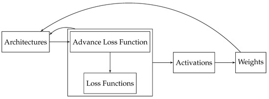
Figure 3.
Model choice method scheme.
For the purpose of controlling and processing this experiment, three python packages were created.
- Alquimodelia (https://github.com/alquimodelia, accessed on 9 March 2025): A Keras-based model builder package to create the necessary models with each different arch and variable;
- Alquitable (https://github.com/alquimodelia/alquitable, accessed on 9 March 2025): A Keras-based workshop package to create custom callbacks, loss functions, data generators;
- MuadDib (https://github.com/alquimodelia/MuadDib, accessed on 9 March 2025): A machine learning framework that uses Alquimodelia to test and choose the best models on given conditions automatically.
The experiments were performed using Keras >= 3, a high-level deep learning library that simplifies the implementation of neural networks, with a torch backend on a CPU laptop.
4.2. Metrics
With distinct weights, the metrics are used to choose the best model on each iteration, and they can be divided into the following two groups:
- Model metrics, where we just use the usual regression metrics, adding a metric for how much the model missed in allocating for the validation period;
- Comparative metrics, where we assert percentage gains over the current allocation method.
4.2.1. Model Metrics
Different metrics have been considered to evaluate the model outputs, such as Root Mean Square Error (RMSE) and Sum of Absolute Errors (SAE):
where t is the observed value, p is the forecast, and n is the number of samples.
SAE can be divide into the following metrics, where we obtain the error, within the time period, of allocated energy not enough for the needs and too much energy allocated separately.
The missing allocation (AllocM) is computed as follows:
The surplus allocation (AllocS) is computed as follows:
These metrics are needed to obtain a better error than the benchmark, but also to have less wasted AllocM and fewer occurrences of AllocS.
4.2.2. Model/Benchmark Comparative Metrics
Performance Percentage Gain (PPG) is the percentage of how much better is the model over the benchmark; it is computed as follows:
The following metrics are the same but for only missing allocation and surplus allocation.
Performance Percentage Gain Missing (PPGM) computes the performance of the missing allocation as follows:
Performance Percentage Gain Surplus (PPGS) computes the performance of the surplus allocation as follows:
The PPGPositive metric shows how much better is the model over the benchmark, but only if PPGM and PPGM are positive.
5. Case Study
To evaluate the applicability of machine learning techniques to secondary reserve allocation, this study was conducted using the Spanish electricity market historical data from 2014 to 2024, with 2014 to 2023 being the training period.
5.1. Data Sources and Preprocessing
This study aims at minimizing the difference between allocated capacity and used energy in the Spanish secondary reserve market.
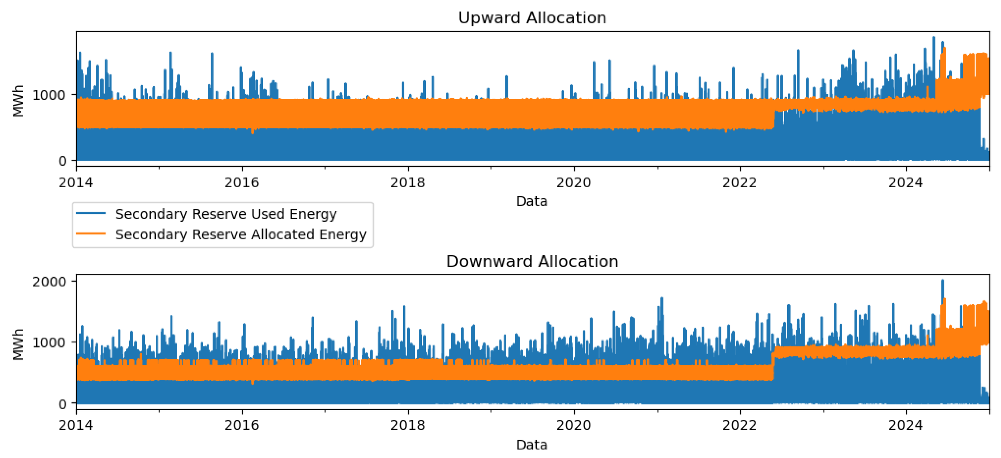
Figure 4 presents the data of the allocated upward and downward capacity and the used energy.

Figure 4.
Spanish allocated upward and downward secondary capacity and used energy.
The significant difference between allocated capacity and used energy can be verified from Figure 4. The blue area bellow the orange area reflects the excess of allocated capacity. Contrariwise, the blue area above the orange area reflects the missing allocated capacity. From the figure, it can be verified that the incidence of excess allocated capacity is significantly higher than the incidence of missing allocated capacity. Historically, excess allocated capacity was more common for upward capacity and excess missing energy for downward capacity. However, the Spanish TSO changed the methodology in the middle of 2022 because of the European gas crisis, increasing the allocation of downward capacity to a value practically symmetrical to upward capacity. Furthermore, after the gas crisis, an increase in the number of events with missing energy can be verified, supporting the use of dynamic sizing of secondary capacity. Indeed, because of that, the TSO changed the methodology in the middle of 2024 to decrease the number of missing energy events. Now, the deterministic methodology is more dynamic throughout the day, reducing the quantity of missing energy. However, it substantially increased the practically symmetrical allocated upward and downward capacity, highly increasing the unused extra capacity.
The case study utilizes publicly available operational and historical data from the Spanish TSO, REE (please check the Data Availability Statement). The dataset includes the key variables presented in Table 2.
Table 2.
ESIOS data used in the study.
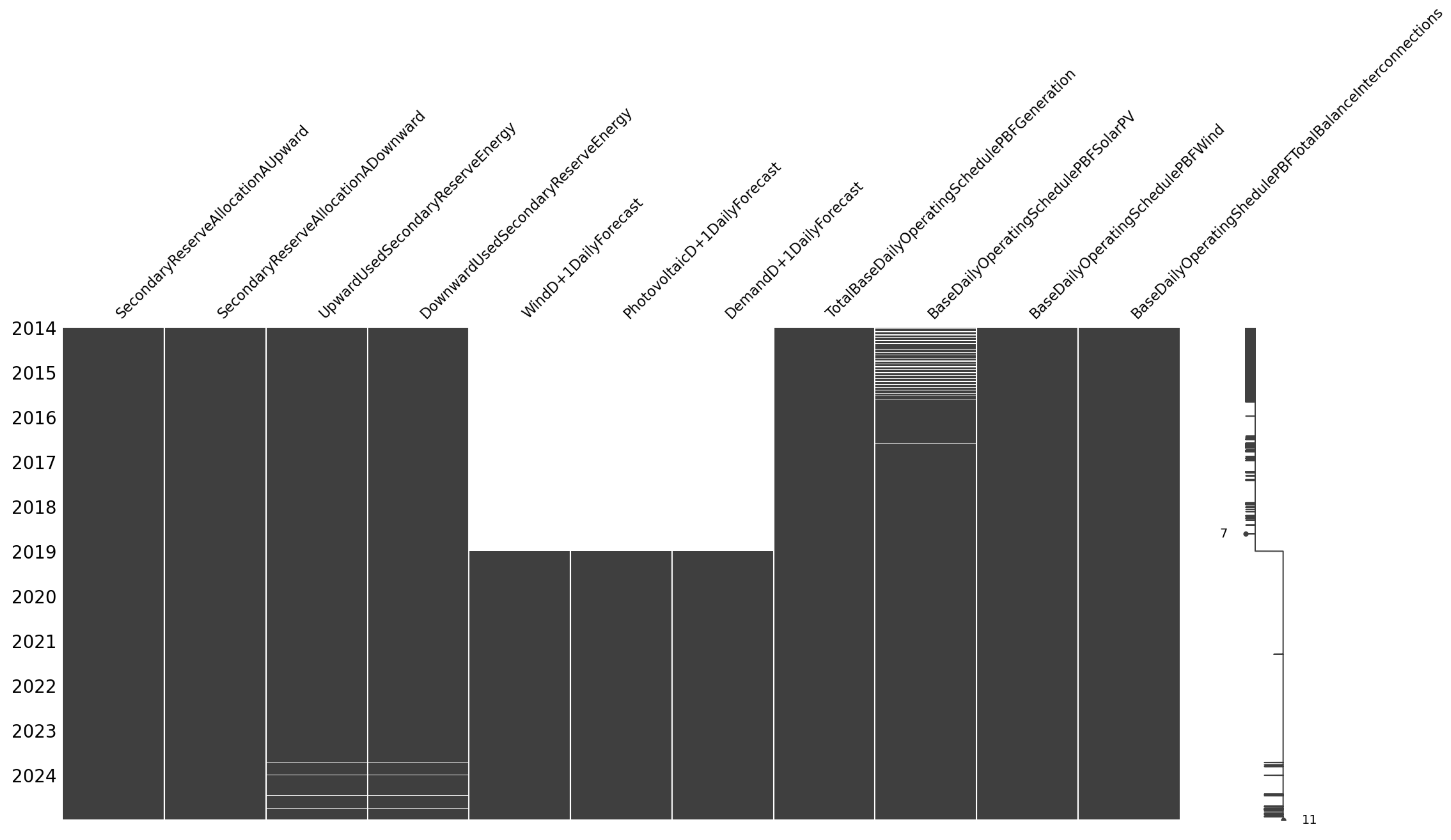
The data span multiple years to account for seasonal variability and long-term trends in vRES generation and demand. Data preprocessing only handled missing values using interpolation methods, with IterativeImputer (see Supplementary Material) [35,36], as presented in Figure 5.
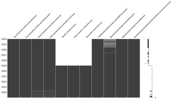
Figure 5.
Missing data per attribute timewise.
To choose the temporal space of the models, temporal auto-correlations were checked in Table 3.
Table 3.
Temporal self-correlation.
From Table 3, small correlations between variables can be verified.
The goal is to forecast DA values 24 h ahead. The input for that forecast considers that temporal correlations present 168 h after each day as the next correlation, which represents a week; i.e., it used the data of a week to forecast the next day. Variables have been added to account for each time range: day, day of year, month, and day of week.
Therefore, models will receive data in (Batch Size, 168, 18) shape for input and (Batch Size, 24, 1) shape for output.
5.1.1. Training Data
For training the full dataset from 2014 to 2023, the data used have the following summary presented in Table 4:
Table 4.
Training data summary.
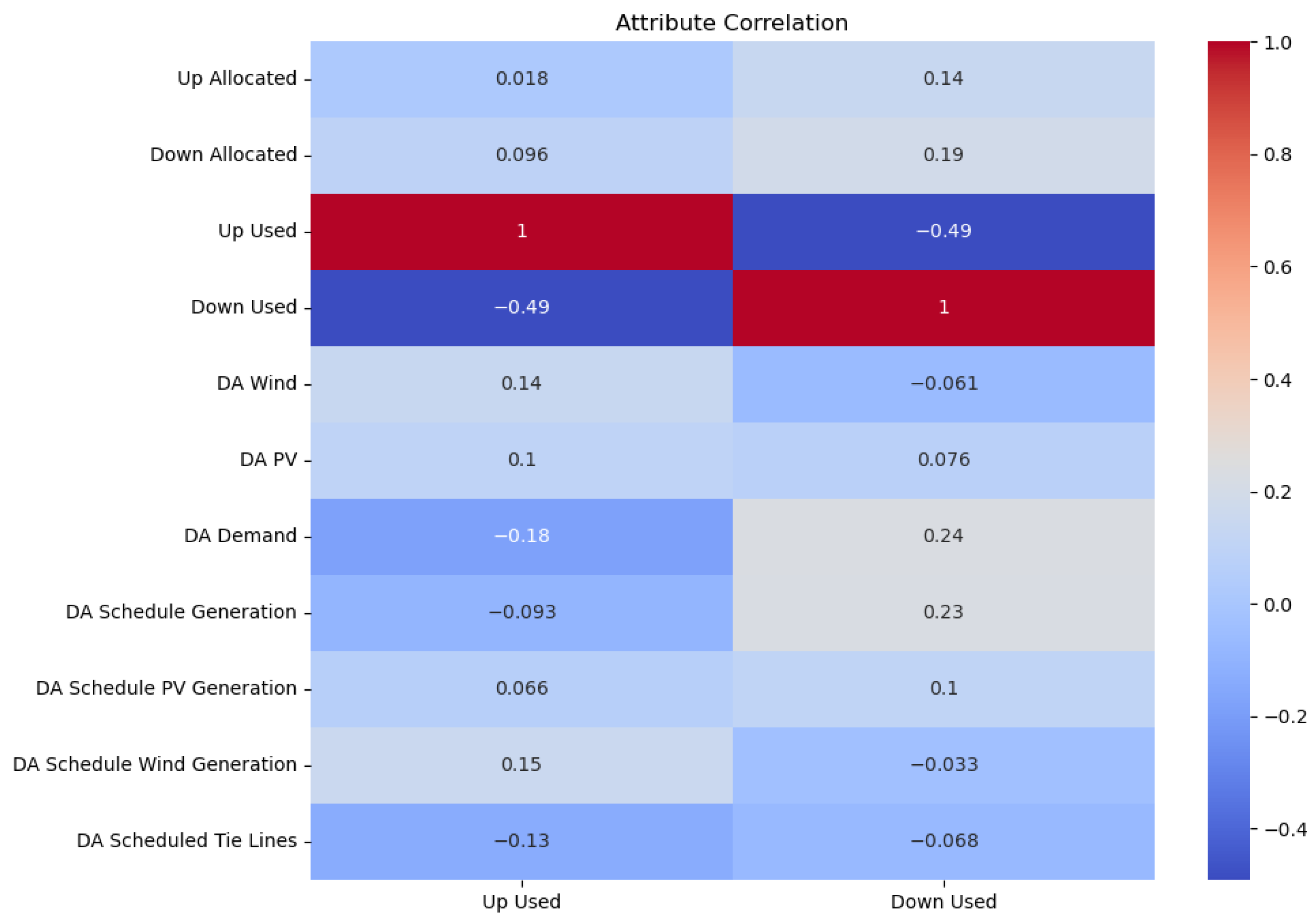
Significant standard deviations between the used energy for up and that for down regulation can be verified. Furthermore, even the allocated up and down capacities significantly differ according to the time period. The correlation of each variable with used secondary reserve energy is presented in Figure 6.
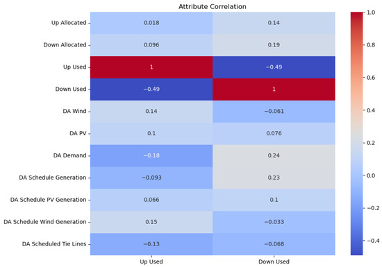
Figure 6.
Attribute correlation to variables to forecast.
In Figure 6, it is possible to verify that the correlation between allocated capacities and used energy is close to zero.
The goal of this work is to reduce the difference between allocated capacities and used energy to efficiently use the available resources.
5.1.2. Validation Data
As regards validation, the year 2024 was chosen, with a summary presented in Table 5.
Table 5.
Validation data summary.
Using the noncomparative metrics, the results are presented in Table 6.
Table 6.
Metric results for validation data.
Table 6 presents the main problems of the actual capacity allocation methodology, resulting in high (i) errors (RMSE and SAE) with used energy, (ii) missing energy (AllocM), and (iii) extra energy (AllocS).
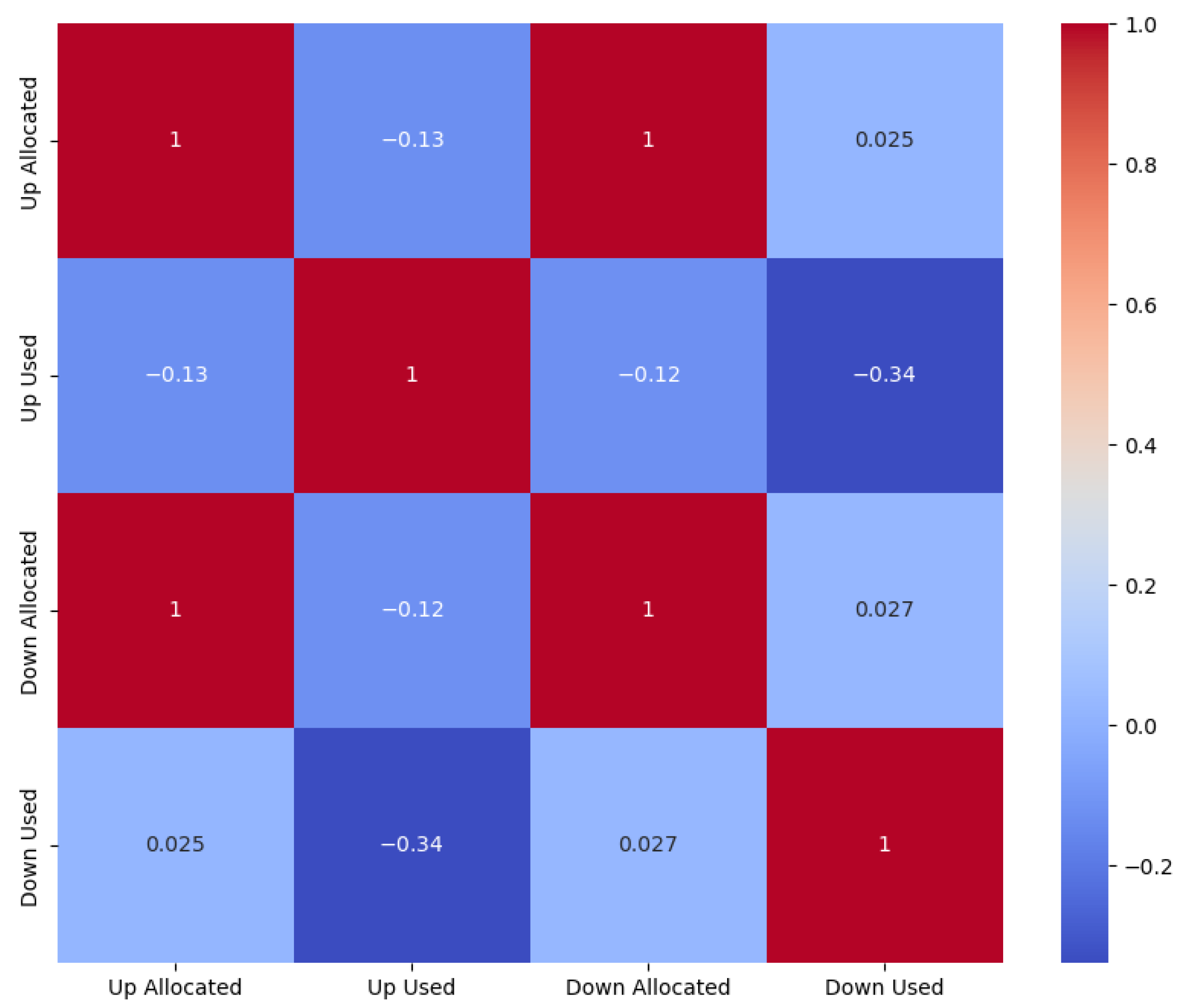
The correlation of allocated energy in the current method to the used energy can be seen in Figure 7.
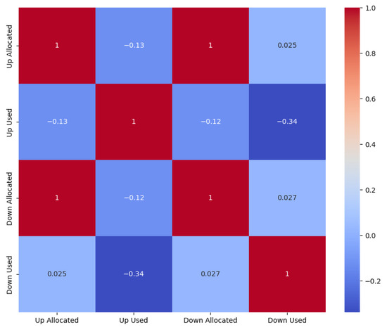
Figure 7.
Attribute correlation benchmark.
In Figure 7, a high correlation between up and down allocated capacities can be verified, identifying the practically symmetrical used allocation. Furthermore, the correlation of allocated capacities with used energy is small, which can be solved by using dynamic allocation as presented in the next section.
5.2. Results
The best results, only based on PPG Positive, for each architecture are presented in Table 7 and Table 8, where Vanilla means it is only one layer deep, and Stacked means two layers deep.
Table 7.
Metric results for up and down forecast.
Table 8.
Comparative metric results for up and down forecast.
To choose the best model, there was analysis on PPG and the individuals PPGS and PPGM. This was so that the final results would not just be the one best across the validation time, but also mean-wise at the same time.
Table 9.
Best model variable description.
Table 10.
Model metric results for predictions.
Table 11.
Model/benchmark comparative metrics results for predictions.
When comparing Table 6 with Table 10, a significant improvement in all outputs can be verified, supported by the metrics presented in Table 11. Indeed, by using the best machine learning methodology, in Table 11, it is possible to verify a reduction of 21.92% and 11.39% in the extra up and down allocated capacity (PPGS) concerning the benchmark, respectively. Furthermore, the missing allocated up and down capacity (PPGM) also decreased by 1.24% and 9.31% concerning the benchmark, respectively.
Table 12 presents the overall description and comparison of the presented model with the benchmark.
Table 12.
Model results and (allocated) values within 2024.
The proposed model presents an overall improvement of ~22% in upward allocation and ~11% in downward allocation, compared with current allocation methods.
The hourly mean differences between benchmark and validation results are presented in Table 13.
Table 13.
Mean % between model and benchmark.
The average hourly improvements are ~16% and ~9%, respectively, which also is an improvement on state of the art [20] with 13% and 8%. The current study can free on average ~12% of hourly resources, lowering the need to allocate down and up capacity to the secondary reserve by ~21% and ~11%, respectively.
It can also be checked that the correlation between used and allocated is bigger than in the current method, achieving 36% in both upward energy and downward energy, as presented in Figure 8.
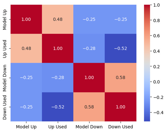
Figure 8.
Correlations between used and allocated energy.
5.3. Discussion and Shortcomings
Although the gain between this method and the literature [20] is small, this study shows that machine learning techniques can, with lower effort, obtain the same or better response than more traditional methods.
Since the main goal was to insert machine learning studies in the area, compared with other techniques, the same set of variables has been used and has expanded the dataset, in time, as much as it was available.
With this, it can also be inferred that feature selection would be an improvement on the current model, and specially using only consumption and production variables, instead of DA forecasts, leaving the forecast alone to the model. A study on feature selection might provide greater insight on which best variables can be used to model the forecast in hand.
A future study might also prove that only the use of recent data could provide better insight on current modulation, without the bias of older energy schemes.
Given also the current dynamic state of machine learning techniques, the best architectures to provide the best forecast might come from families different from the one used in this study.
As regards structure, it might be better to create a model for every single different hour, instead of a model for the 24 h, or even a single hour, model, but for all hours.
All these choices impact the feasibility of the final results and should be made considering the production level on where they will be used.
6. Conclusions
The results of the case study validate the effectiveness of machine learning techniques in improving the accuracy of reserve forecasts and optimizing reserve allocation. By dynamically adjusting upward and downward reserves based on real-time forecasts, the proposed methodology addresses the inefficiencies of static procurement methods. The observed cost savings and improved reserve utilization demonstrate the practical benefits of this approach for systems with high renewable penetration.
Additionally, the case study highlights the potential for asymmetrical dynamic reserve procurement to better reflect system needs, particularly during periods of extreme renewable generation variability. The integration of weather forecasts into the predictive models further enhances their reliability, ensuring that reserve procurement decisions are informed by real-time conditions.
Using the StackedFCNN architecture, the average hourly improvements are ~16% and ~9%, respectively. By using this learning architecture, the average hourly secondary allocated capacity can be reduced by ~12%, lowering the hourly need to allocate down and up capacities by ~11% and ~21%, respectively.
In conclusion, the case study illustrates that dynamic reserve procurement, supported by machine learning techniques, can significantly improve the efficiency and cost-effectiveness of balancing services in modern electricity systems. These findings provide a strong foundation for further research and potential implementation in other balancing markets with similar challenges.
For future work, a daily operational machine learning methodology will be developed, considering daily training data updates to better correlate reserved capacity with real-time reserve needs.
Supplementary Materials
All methodologies are provided to allow the replicability of this work and testing on other markets. An IterativeImputer data preprocessing methodology is at https://scikit-learn.org/stable/modules/generated/sklearn.impute.IterativeImputer.html, accessed on 9 March 2025. An Alquimodelia model can be obtained at https://github.com/alquimodelia, accessed on 9 March 2025. A mirror weights ratio methodology is at https://github.com/alquimodelia/alquitable/blob/main/alquitable/advanced_losses.py#L33, accessed on 9 March 2025. An Alquitable workshop package is at https://github.com/alquimodelia/alquitable, accessed on 9 March 2025. A MuadDib machine learning framework can be obtained from https://github.com/alquimodelia/MuadDib, accessed on 9 March 2025.
Author Contributions
Conceptualization, J.P.d.S. and H.A.; methodology, J.P.d.S. and H.A.; software, J.P.d.S.; validation, H.A.; formal analysis, J.P.d.S. and H.A.; investigation, J.P.d.S. and H.A.; resources, J.P.d.S. and H.A.; data curation, J.P.d.S. and H.A.; writing—original draft, J.P.d.S.; writing—review and editing, H.A.; visualization, J.P.d.S.; supervision, H.A.; project administration, H.A.; funding acquisition, H.A. All authors have read and agreed to the published version of the manuscript.
Funding
This work received funding from the EU Horizon 2020 research and innovation program under the project TradeRES (grant agreement no. 864276).
Data Availability Statement
The data used to dynamically forecast secondary reserve needs and validate the proposed model are available at https://www.esios.ree.es/en, accessed on 9 March 2025.
Conflicts of Interest
The authors declare no conflicts of interest.
Abbreviations
| aFRR | automatic Frequency Restoration Reserve |
| AllocM | missing allocation |
| AllocS | surplus allocation |
| CNN | convolutional neural network |
| DA | Day-Ahead |
| DAM | day-ahead markets |
| ENTSO-E | European Network of Transmission System Operators for Electricity |
| ESIOS | Sistema de Información del Operador del Sistema |
| FCNN | Fully Connected Neural Network |
| FCR | Frequency Containment Reserve |
| GELU | Gaussian Error Linear Unit |
| IDM | intraday markets |
| LSTM | Long Short-Term Memory |
| MAE | Mean Absolute Error |
| mFRR | manual Frequency Restoration Reserve |
| MIBEL | Iberian Market of Electricity |
| MSE | Mean Squared Error |
| MSLE | Mean Squared Logarithmic Error |
| OMIE | Operador del Mercado Ibérico de Energía—Pólo Espanhol, S.A |
| OMIP | Operador do Mercado Ibérico de Energia Português |
| PPG | Performance Percentage Gain |
| PPGM | Performance Percentage Gain Missing |
| PPGS | Performance Percentage Gain Surplus |
| PV | solar photovoltaic |
| REE | Red Eléctrica de España |
| RMSE | Root Mean Square Error |
| ReLU | Rectified Linear Unit |
| REN | Redes Energéticas Nacionais |
| SAE | Sum of Absolute Errors |
| SDG | Sustainable Development Goals |
| TSO | Transmission System Operators |
| vRES | variable Renewable Energy Systems |
| Indices | |
| i | hour |
| n | number of samples |
| Parameters | |
| hourly ratio | |
| empiric coefficients | |
| Variables | |
| maximum consumption | |
| secondary energy forecast | |
| R | secondary control reserve |
| secondary energy observed |
References
- Maris, G.; Flouros, F. The Green Deal, National Energy and Climate Plans in Europe: Member States’ Compliance and Strategies. Adm. Sci. 2021, 11, 75. [Google Scholar] [CrossRef]
- Franc-Dabrowska, J.; Madra-Sawicka, M.; Milewska, A. Energy Sector Risk and Cost of Capital Assessment—Companies and Investors Perspective. Energies 2021, 14, 1613. [Google Scholar] [CrossRef]
- Perissi, I.; Jones, A. Investigating European Union Decarbonization Strategies: Evaluating the Pathway to Carbon Neutrality by 2050. Sustainability 2022, 14, 4728. [Google Scholar] [CrossRef]
- Dobrowolski, Z.; Drozdowski, G.; Panait, M.; Apostu, S.A. The Weighted Average Cost of Capital and Its Universality in Crisis Times: Evidence from the Energy Sector. Energies 2022, 15, 6655. [Google Scholar] [CrossRef]
- Ocker, F.; Ehrhart, K.M. The “German Paradox” in the balancing power markets. Renew. Sustain. Energy Rev. 2017, 67, 892–898. [Google Scholar] [CrossRef]
- Frade, P.M.; Pereira, J.P.; Santana, J.J.; Catalão, J.P. Wind balancing costs in a power system with high wind penetration—Evidence from Portugal. Energy Policy 2019, 132, 702–713. [Google Scholar] [CrossRef]
- Prema, V.; Bhaskar, M.S.; Almakhles, D.; Gowtham, N.; Rao, K.U. Critical Review of Data, Models and Performance Metrics for Wind and Solar Power Forecast. IEEE Access 2022, 10, 667–688. [Google Scholar] [CrossRef]
- Shahidehpour, M.; Yamin, H.; Li, Z. Market Operations in Electric Power Systems. In Market Operations in Electric Power Systems; Wiley-IEEE Press: Hoboken, NJ, USA, 2002. [Google Scholar] [CrossRef]
- Strbac, D.S.K.G. Fundamentals of Power System Economics, 2nd ed.; John Wiley & Sons: Chichester, UK, 2018. [Google Scholar]
- Algarvio, H.; Lopes, F.; Couto, A.; Estanqueiro, A.; Santana, J. Variable Renewable Energy and Market Design: New Products and a Real-World Study. Energies 2019, 12, 4576. [Google Scholar] [CrossRef]
- Skytte, K.; Bobo, L. Increasing the value of wind: From passive to active actors in multiple power markets. Wiley Interdiscip. Rev. Energy Environ. 2019, 8, e328. [Google Scholar] [CrossRef]
- Miettinen, J.; Holttinen, H. Impacts of wind power forecast errors on the real-time balancing need: A Nordic case study. IET Renew. Power Gener. 2019, 13, 227–233. [Google Scholar] [CrossRef]
- Martín-Martínez, S.; Lorenzo-Bonache, A.; Honrubia-Escribano, A.; Cañas-Carretón, M.; Gómez-Lázaro, E. Contribution of wind energy to balancing markets: The case of Spain. Wiley Interdiscip. Rev. Energy Environ. 2018, 7, e300. [Google Scholar] [CrossRef]
- Algarvio, H.; Lopes, F.; Couto, A.; Estanqueiro, A. Participation of wind power producers in day-ahead and balancing markets: An overview and a simulation-based study. Wiley Interdiscip. Rev. Energy Environ. 2019, 8, e343. [Google Scholar] [CrossRef]
- Algarvio, H.; Couto, A.; Estanqueiro, A. RES.Trade: An Open-Access Simulator to Assess the Impact of Different Designs on Balancing Electricity Markets. Energies 2024, 17, 6212. [Google Scholar] [CrossRef]
- Frade, P.M.; Osório, G.J.; Santana, J.J.; Catalão, J.P. Regional coordination in ancillary services: An innovative study for secondary control in the Iberian electrical system. Int. J. Electr. Power Energy Syst. 2019, 109, 513–525. [Google Scholar] [CrossRef]
- Knorr, K.; Dreher, A.; Böttger, D. Common dimensioning of frequency restoration reserve capacities for European load-frequency control blocks: An advanced dynamic probabilistic approach. Electr. Power Syst. Res. 2019, 170, 358–363. [Google Scholar] [CrossRef]
- Vos, K.D.; Stevens, N.; Devolder, O.; Papavasiliou, A.; Hebb, B.; Matthys-Donnadieu, J. Dynamic dimensioning approach for operating reserves: Proof of concept in Belgium. Energy Policy 2019, 124, 272–285. [Google Scholar] [CrossRef]
- Kruse, J.; Schäfer, B.; Witthaut, D. Secondary control activation analysed and predicted with explainable AI. Electr. Power Syst. Res. 2022, 212, 108489. [Google Scholar] [CrossRef]
- Algarvio, H.; Couto, A.; Estanqueiro, A. A Methodology for Dynamic Procurement of Secondary Reserve Capacity in Power Systems with Significant vRES Penetrations. In Proceedings of the 2024 20th International Conference on the European Energy Market (EEM), Istanbul, Turkey, 10–12 June 2024. [Google Scholar] [CrossRef]
- Handbook, U.O. Policy 1: Load-frequency control and performance. Final. Policy 2009, 2, P1-1–P1-32. [Google Scholar]
- Cardo-Miota, J.; Pérez, E.; Beltran, H. Deep learning-based forecasting of the automatic Frequency Reserve Restoration band price in the Iberian electricity market. Sustain. Energy Grids Netw. 2023, 35, 101110. [Google Scholar] [CrossRef]
- Grubb, M.; Drummond, P.; Maximov, S. Separating Electricity from Gas Prices Through Green Power Pools: Design Options and Evolution; Institute for New Economic Thinking Working Paper Series; UCL Institute for Sustainable Resources: London, UK, 2022; Volume 193. [Google Scholar]
- Frade, P.M.; Shafie-khah, M.; Santana, J.J.; Catalão, J.P. Cooperation in ancillary services: Portuguese strategic perspective on replacement reserves. Energy Strategy Rev. 2019, 23, 142–151. [Google Scholar] [CrossRef]
- Papavasiliou, A. An overview of probabilistic dimensioning of frequency restoration reserves with a focus on the greek electricity market. Energies 2021, 14, 5719. [Google Scholar] [CrossRef]
- Khodadadi, A.; Herre, L.; Shinde, P.; Eriksson, R.; Soder, L.; Amelin, M. Nordic Balancing Markets: Overview of Market Rules. In Proceedings of the 2020 17th International Conference on the European Energy Market (EEM), Stockholm, Sweden, 16–18 September 2020. [Google Scholar] [CrossRef]
- Couto, A.; Estanqueiro, A. Assessment of wind and solar PV local complementarity for the hybridization of the wind power plants installed in Portugal. J. Clean. Prod. 2021, 319, 128728. [Google Scholar] [CrossRef]
- Benti, N.E.; Chaka, M.D.; Semie, A.G. Forecasting Renewable Energy Generation with Machine Learning and Deep Learning: Current Advances and Future Prospects. Sustainability 2023, 15, 7087. [Google Scholar] [CrossRef]
- Hunt, S.; Shuttleworth, G. Competition and Choice in Electricity; John Wiley & Sons: Chichester, UK, 1998. [Google Scholar]
- Liu, Z.; Mao, H.; Wu, C.Y.; Feichtenhofer, C.; Darrell, T.; Xie, S. A ConvNet for the 2020s. In Proceedings of the 2022 IEEE/CVF Conference on Computer Vision and Pattern Recognition (CVPR), New Orleans, LA, USA, 18–24 June 2022; pp. 11966–11976. [Google Scholar] [CrossRef]
- Costa, R.L.d.C. Convolutional-LSTM networks and generalization in forecasting of household photovoltaic generation. Eng. Appl. Artif. Intell. 2022, 116, 105458. [Google Scholar] [CrossRef]
- Hewamalage, H.; Bergmeir, C.; Bandara, K. Recurrent Neural Networks for Time Series Forecasting: Current status and future directions. Int. J. Forecast. 2021, 37, 388–427. [Google Scholar] [CrossRef]
- Shelhamer, E.; Long, J.; Darrell, T. Fully Convolutional Networks for Semantic Segmentation. IEEE Trans. Pattern Anal. Mach. Intell. 2014, 39, 640–651. [Google Scholar] [CrossRef] [PubMed]
- Vaswani, A.; Shazeer, N.; Parmar, N.; Uszkoreit, J.; Jones, L.; Gomez, A.N.; Kaiser, Ł.; Polosukhin, I. Attention Is All You Need. In Proceedings of the 31st Conference on Neural Information Processing Systems (NIPS 2017), Long Beach, CA, USA, 4–9 December 2017; pp. 5999–6009. [Google Scholar]
- van Buuren, S.; Groothuis-Oudshoorn, K. mice: Multivariate Imputation by Chained Equations in R. J. Stat. Softw. 2011, 45, 1–67. [Google Scholar] [CrossRef]
- Buck, S.F. A Method of Estimation of Missing Values in Multivariate Data Suitable for use with an Electronic Computer. J. R. Stat. Soc. Ser. B (Methodol.) 1960, 22, 302–306. [Google Scholar] [CrossRef]


Disclaimer/Publisher’s Note: The statements, opinions and data contained in all publications are solely those of the individual author(s) and contributor(s) and not of MDPI and/or the editor(s). MDPI and/or the editor(s) disclaim responsibility for any injury to people or property resulting from any ideas, methods, instructions or products referred to in the content. |
© 2025 by the authors. Licensee MDPI, Basel, Switzerland. This article is an open access article distributed under the terms and conditions of the Creative Commons Attribution (CC BY) license (https://creativecommons.org/licenses/by/4.0/).