Flow Management in High-Viscosity Oil–Gas Mixing Systems: A Study of Flow Regimes

Abstract

The flow management of the gas–liquid mixture module is crucial for the transmission efficiency of crude oil-and-natural gas-gathering and transportation systems. The concurrent flow of high-viscosity crude oil and natural gas in gas–liquid mixing is investigated numerically by adopting an improved volume of fluid (VOF) model programmed with the OpenFOAM v2012 software package. Over a wide range of superficial velocities for the oil, from 0.166 to 5.529 m/s, and natural gas, from 0.138 to 27.645 m/s, a variety of flow regimes of bubble flow, plug flow, slug flow, and annular flow are encountered successively, which are essentially consistent with the Brill and Mandhane flow regime identification criteria. The results show that the oil volume fraction, fluid velocity, and bubble slip velocity together affect the growth of bubbles in the pipeline at a low gas velocity. In the case of slug flow, the phenomenon of liquid film plugging is noticeable, and the flow is very unstable, which should be avoided as much as possible. Nonetheless, it is commended that stable plug flow and annular flow with a high oil transportation efficiency and minimal power consumption are friendly working conditions.

1. Introduction

Despite challenges arising from climate change and the greenhouse gas effect, fossil fuels such as natural gas and crude oil are still widely used as one of the main energy sources and will continue to be used in the coming decades because of relatively economical transportation modes and accessible consumer infrastructure. With the depletion of conventional oil and gas resources, heavy oil with high viscosity plays one of the most important alternative roles in the future energy supply [1]. To reduce the consumption of oil and gas transportation, the energy-saving design of oil and gas transportation systems can effectively improve the comprehensive economic benefits of this energy source.

Oil-and-gas mixed transportation in gathering pipelines, which delivers resources between the point of extraction and the relevant processing location, is considered a kind of energy-saving technology in China’s oil and gas storage and transportation industry in recent years because the energy consumption and pipe material expenditures of this system are greatly reduced compared to traditional methods [2]. Specifically, oil-and-gas-gathering systems consist of flowlines connected to a production manifold and process facilities that move fluids (oil, gas, water, and solids) to be processed from wells to a main processing plant. Usually, in order to inspect and control production in a gathering system (as shown in Figure 1), the oil-and-gas mixture from the production manifold is vented to a separator, where gas content and liquids are completely isolated, while some solid impurities are roughly drained. The separated gas and liquids, including crude oil with some water cut, are gauged by gas and liquid flowrate meters, respectively. Before being injected into the gathering pipelines, they are driven by the compressors and the pump, respectively, into a specially designed mixer to a concurrent gas–liquid two-phase flow.

Oil and natural gas are two substances in different phases, which produce different flow regimes when mixed and transported simultaneously. When the flow parameters are within a specific range of velocities, different flow regimes will occur, such as an intermittent slug flow, which will cause the pipeline system to diverge or become unstable [3,4]. Flutter instability and other phenomena seriously threaten the safe operation of these pipeline systems [5,6]. Therefore, studying the flow management of oil and natural gas during mixed transportation is of great significance for system safety, operational stability, and reducing pump power loss.

Accurately identifying the flow characteristics of high-viscosity oil–gas two-phase fluids during experimentation presents a significant challenge. Baba et al. [7] conducted experimental studies on high-viscosity oil–air two-phase flow, employing a fast-sampling gamma densitometer to measure slug length. The study revealed that the length of the slug is highly sensitive to the viscosity of the liquid. An experiment of heavy oil–water–gas in the vertical tube was carried out by Liu et al. [8], in which various flow regimes, such as bubble, slug, churn, and annular flows, were observed, and then the method of calculating the friction pressure gradient was revealed. Khaledi et al. [1] conducted an experimental study on velocity and pressure testing of high-viscosity oil and gas through various flow regimes, such as bubble flow, the transition process of stratified flow and slug flow, in a pipe with an inner diameter of 69 mm. In order to accurately calibrate the water content of oil–gas–water multiphase flow, Chen et al. [9] designed a vertical tube experiment using a measurement system with a double-ring conductivity probe and a double-helical capacitance probe, but there was still a large uncertainty of measurement for the bubble flow. Wang et al. [10] used a new type of liquid film sensor by introducing entropy analysis to study the structural characteristics of Taylor bubbles in the mixed flow of gas–oil–water. The study revealed that the thickness of the liquid film is correlated with the superficial velocities of both the liquid and gas phases, as well as the oil content. Chang et al. [11] employed electrical capacitance volume tomography (ECVT) technology to construct phase interface models for the experimental investigation of the slugging behavior in gas–liquid two-phase flow within long-distance pipelines, leading to the development of an improved model for predicting severe slugs. Li et al. [12] employed the hypergraph-based global–local structure analysis (HGLSA) method to monitor information from oil–gas–water flow experiments. Additionally, they conducted a multiscale characterization of the flow using Hilbert–Huang transform and multiscale robust empirical permutation entropy (Ms-rePE) analysis. Given the difficulty in measuring two-phase flow, accurately predicting flow distribution in industrial applications through experimental methods becomes a challenging task.

Due to the difficulty in handling the interphase variations in multiphase flow and the complexity of momentum interactions, numerical simulations remain highly challenging [13]. In the 1970s, researchers from various countries proposed several numerical methods for classifying flow regime boundaries. The Mandhane criterion [14] and the Brill criterion [15] are commonly used methods to discriminate gas–liquid two-phase flow. The Mandhane criterion, which focuses on the superficial velocities of oil and gas, is one of the most widely used methods for determining gas–liquid two-phase flow regimes. Meanwhile, Brill [15] used air–kerosene and air–lubricating oil as the working fluid to conduct experiments on the influence of inclination angle, eventually proposing the Brill criterion for assessing the flow regime. However, these methods overlook the effects of pipeline structure and fluid viscosity and do not provide a direct visual representation of flow regimes. Taitel and Dukler et al. [16,17] adopted Kelvin–Helmholtz instability theory to predict the conversion conditions of layered flow and non-layered flow in the two-phase flow in a tube, which has become a typical example of the stability theory applied to the study of two-phase flow regimes. Lin et al. [18] used the viscous long-wave instability theory to study the viscosity of liquids. Their results show that, when fluid instability occurs, the interfacial wave velocity is greater than the average flow rate of the liquid, and the slug flow develops from the long wave. Shaaban and Al-Safran [19] analyzed experimental data from 1904 high-viscosity slug lengths and developed a mechanistic model for slug length, which considers both mass and momentum conservation. Upon validation, the model exhibited an absolute average percentage error of 34%. It can be seen that these theoretical studies still have some errors and test uncertainties. In CFD numerical simulation, Padoin et al. [20] used the volume of fluid (VOF) model to calculate the influence of wall wettability on air–water flow in microchannel tubes, confirming the reliability of CFD calculation and evaluation. Yan and Che [21] coupled the interface tracking method and two-fluid model to calculate the complex multiphase flow generated when the large-scale gas–liquid interface and the small-scale gas–liquid interface exist at the same time and used the VOF/PLIC method to evaluate the movement of the large-scale interface. Nieves-Remacha et al. [22] used OpenFOAM software to calculate the influence of contact angle and surface tension on flow regimes in advanced-flow reactor (ATR) technology and pointed out that the geometric reconstruction technology used by the VOF algorithm can handle the two-phase interface faster and better. Nagarajan and Trujillo [23] analyzed the applicability of coupling VOF and RANS (Reynolds-Averaged Navier–Stokes) calculations in OpenFOAM for simulating water-and-oil core annular flow. Li et al. [24] conducted simulation studies on oil–water core annular flow in horizontal pipes. They investigated the numerical accuracy of DNS and RANS models under different conditions, such as unidirectional flow and two-phase flow wave scenarios.

There is still a lack of extensive numerical simulation research on high-viscosity two-phase flow, especially for high-viscosity oil combined with gas. Accurately simulating the two-phase flow of oil and gas can not only provide prediction and verification data for engineering safety design but can also optimize the actual performance of oil-and-gas multiphase flow transportation systems with a small loss of pump power. Furthermore, being an open-source code software, the OpenFOAM software is particularly suitable for dealing with high-viscosity unsteady multiphase flow.

Therefore, the objective of this study is to put forward transportation management schemes for high transportation efficiency and low pressure loss. OpenFOAM is employed to simulate the mixed-flow regime of gas–liquid two-phase flow at different flow rates in a gathering pipe through a specially designed mixer. The effect of a range of flow rates on the flow regime and the ratio of gas-to-liquid content are the object of special focus. The system stability and pump power loss under different oil transportation rates are discussed. It is expected that the finding will provide a reference for the mixed transportation of oil and natural gas.

2. Physical and Mathematical Model

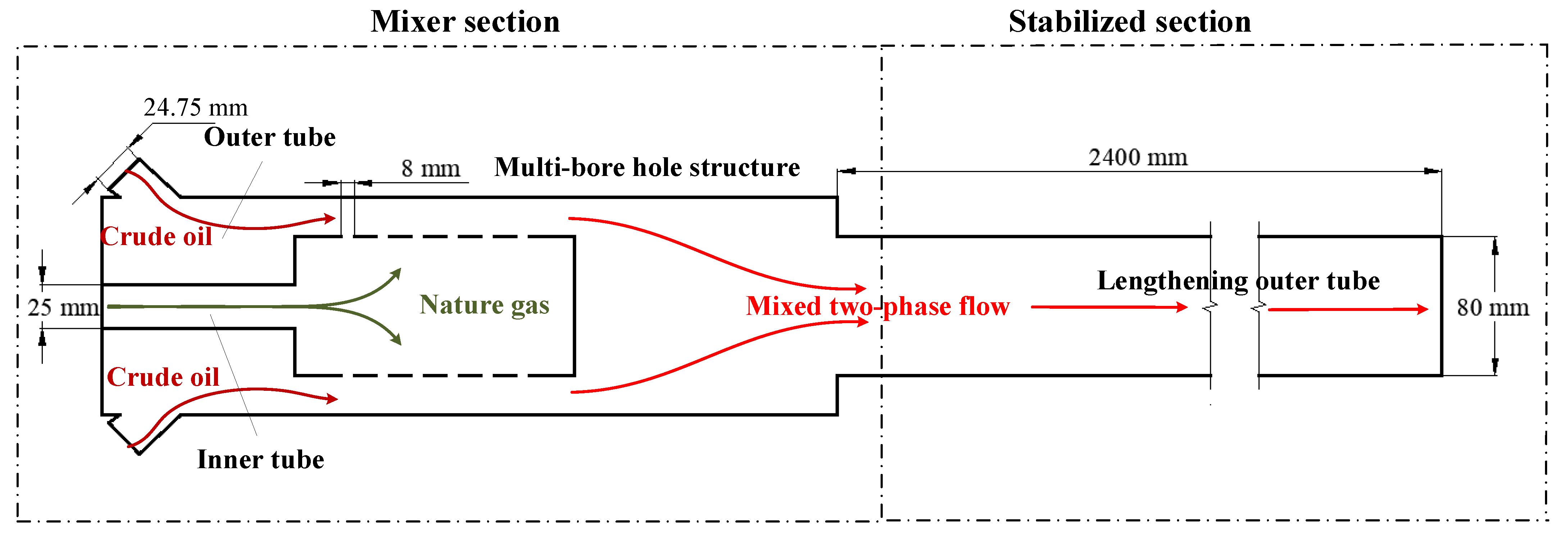
2.1. Physical Model

To investigate the mixing phenomenon of oil and natural gas at different flow rates, the structural design of a gas–liquid mixer, which can be frequently adopted in an oil-and-gas-gathering system, was developed, which is depicted in Figure 2. The mixer prototype consisted of an inner tube and an outer tube with a co-axis. Natural gas and crude oil were injected along the centerline of the inner tube and the circumference of the outer tube, respectively, into the annular space between them to mix and entrain simultaneously to a gas–liquid flow. On the wall of the inner tube, 12 holes with a diameter of 8 mm were drilled to disperse the gas phase and rectify the flow in order to restrain flow vibration and noise. The multi-bore hole structure was chosen on the assumption that the perforated orifice plate was noticeably better than the single-hole orifice plate in terms of the resistance loss and turbulent flow stability [25]. In order to attain a stable and fully developed flow regime under different superficial velocities [26], the outer tube was longer than the inner one. The lengthier outer tube was designated as the stabilized section at the rear end of the mixer, the length of which was 30 times the size of its diameter [27]. Since there were no significant pressure fluctuations within the system, this study did not consider gas penetration and release into the oil.

2.2. Governing Equations

There was a gas–liquid interface in the oil–natural gas two-phase flow in the horizontal tube, the motion of which was dependent on gravity, surface tension, turbulent dissipative forces, and shear forces generated by velocity differences. The volume of fluid (VOF) model, developed by Hirt and Nichols [28] for simulating incompressible two-phase flows with free surfaces, involves solving the transport equation alongside the mass, momentum, and phase function equations simultaneously.

The continuity equation and momentum equation of a two-phase flow are as follows:

$${\displaystyle \frac{\partial \rho }{\partial t}}+\nabla \text{·}(\rho \mathit{u})=0$$

(1)

$${\displaystyle \frac{\partial \rho \mathit{u}}{\partial t}}+\nabla \text{·}(\rho \mathit{u}\mathit{u})=-\nabla p+\nabla \cdot \mathit{\tau }+\rho \mathbf{g}+{\mathit{F}}_{\sigma }$$

(2)

where ρ is the density of the fluid, kg·m⁻³; u is the velocity vector, m·s⁻¹; t is the time, s; p is the pressure, Pa; g is the gravitational acceleration, m·s⁻²; and F_σ represents the surface tension, N·m⁻³. The shear stress τ is induced by the deformation tensor of viscous fluid, N·m⁻², as follows:

$$\mathit{\tau }=\{\rho (\nu +{\nu }_t)[\nabla \mathit{u}+{(\nabla \mathit{u})}^{\mathsf{T}}]\}$$

(3)

where ν_t is the turbulent viscosity, m²·s⁻¹.

Surface tension F_σ can be calculated by the continuous surface force (CSF) model introduced by Brackbill et al. [29]:

$${\mathit{F}}_{\mathsf{\sigma }}={\displaystyle \frac{\sigma \rho \kappa \nabla \alpha }{\frac{1}{2}({\rho }_{\mathrm{g}}+{\rho }_l)}}$$

(4)

$$\kappa =-\nabla \cdot ({\displaystyle \frac{\nabla \alpha }{\left|\nabla \alpha \right|}})={\displaystyle \frac{1}{\left|\nabla \alpha \right|}}[({\displaystyle \frac{\nabla \alpha }{\left|\nabla \alpha \right|}}\cdot \nabla )\left|\nabla \alpha \right|-(\nabla \cdot \nabla \alpha )]$$

(5)

where σ represents the surface tension coefficient, N·m⁻¹; κ is the mean surface curvature, m⁻¹; ▽α is the gradient of the oil phase volume fraction, m⁻¹; and the subscripts g and l represent the gas phase and liquid phase, respectively.

The proportion of liquid and gas phases in the grid cell can be distinguished using the volume fraction of the oil phase α, which can be expressed as follows:

$$\alpha =\left\{\begin{array}{l}0,\mathrm{f}\mathrm{o}\mathrm{r}\mathrm{p}\mathrm{o}\mathrm{i}\mathrm{n}\mathrm{t}\mathrm{s}\mathrm{b}\mathrm{e}\mathrm{l}\mathrm{o}\mathrm{n}\mathrm{g}\mathrm{i}\mathrm{n}\mathrm{g}\mathrm{t}\mathrm{o}\mathrm{n}\mathrm{a}\mathrm{t}\mathrm{u}\mathrm{r}\mathrm{a}\mathrm{l}\mathrm{g}\mathrm{a}\mathrm{s}\\ 0\text{~}1,\mathrm{f}\mathrm{o}\mathrm{r}\mathrm{p}\mathrm{o}\mathrm{i}\mathrm{n}\mathrm{t}\mathrm{s}\mathrm{a}\mathrm{t}\mathrm{t}\mathrm{h}\mathrm{e}\mathrm{i}\mathrm{n}\mathrm{t}\mathrm{e}\mathrm{r}\mathrm{f}\mathrm{a}\mathrm{c}\mathrm{e}\\ 1,\mathrm{f}\mathrm{o}\mathrm{r}\mathrm{p}\mathrm{o}\mathrm{i}\mathrm{n}\mathrm{t}\mathrm{s}\mathrm{b}\mathrm{e}\mathrm{l}\mathrm{o}\mathrm{n}\mathrm{g}\mathrm{i}\mathrm{n}\mathrm{g}\mathrm{t}\mathrm{o}\mathrm{o}\mathrm{i}\mathrm{l}\end{array}\right.$$

(6)

The density ρ, viscosity μ, and velocity u of a two-phase fluid can be written as follows [24,30]:

$$\rho =(1-\alpha ){\rho }_g+\alpha {\rho }_l$$

(7)

$$\mu =(1-\alpha ){\mu }_g+\alpha {\mu }_l$$

(8)

$$\mathit{u}=(1-\alpha ){\mathit{u}}_{\mathrm{g}}+\alpha {\mathit{u}}_l$$

(9)

The phase function equations of the oil phase and the nature gas phase are defined separately as a two-fluid individual phase:

$${\displaystyle \frac{\partial \alpha }{\partial t}}+\nabla \cdot \left({\mathit{u}}_l\alpha \right)=0$$

(10)

$${\displaystyle \frac{\partial (1-\alpha )}{\partial t}}+\nabla \cdot \left[{\mathit{u}}_g\left(1-\alpha \right)\right]=0$$

(11)

In simulations of high-viscosity fluid flows with large density differences, even minor inaccuracies in tracking phase boundaries can severely affect result reliability. Precise phase distribution modeling becomes vital for correctly estimating surface curvature, which directly determines accurate surface tension computations at the fluid interfaces. To mitigate the blurring of gradients caused by numerical diffusion, the method incorporates an extra convective term into the phase fraction equation (Equation (10)) to suppress the interface ambiguity [31]. The improved phase function equation can be written as follows:

$${\displaystyle \frac{\partial \alpha }{\partial t}}+\mathit{u}\cdot \nabla \alpha +\nabla \cdot \left[\alpha \left(1-\alpha \right){\mathit{u}}_c\right]=0$$

(12)

where u_c is the interface-compression equivalent, m·s⁻¹, which can be written as

$${\mathit{u}}_{\mathrm{c}}=\min [c\left|\mathit{u}\right|,\max (\left|\mathit{u}\right|)]{\displaystyle \frac{\nabla \alpha }{\left|\nabla \alpha \right|}}$$

(13)

When the constant c is equal to zero, it indicates no compression at the interface. A value of c = 1, as used in the current research, ensures conservative compression, whereas values greater than one result in intensified compression effects.

The turbulence model can be calculated using the RAS algorithm [32,33,34], which has a low computational cost and performs well in predicting flows with modest variations. ν_t is obtained from the k-ε model, as follows:

$${\displaystyle \frac{\partial \rho k}{\partial t}}+\nabla \cdot (\rho k\mathit{u})=\nabla \cdot [\rho (\nu +{\displaystyle \frac{{\nu }_{\mathrm{t}}}{{\sigma }_{\mathrm{k}}}})\nabla k]+G-\rho \epsilon$$

(14)

$${\displaystyle \frac{\partial \rho \epsilon }{\partial t}}+\nabla \cdot (\rho \epsilon \mathit{u})=\nabla \cdot [\rho (\nu +{\displaystyle \frac{{\nu }_{\mathrm{t}}}{{\sigma }_{\mathsf{\epsilon }}}})\nabla \epsilon ]+C_1\rho {\displaystyle \frac{\epsilon }{k}}G-C_2\rho {\displaystyle \frac{{\epsilon }^2}{k}}$$

(15)

$${\nu }_{\mathrm{t}}=C_{\mathsf{\mu }}{f}_{\mathsf{\mu }}{\displaystyle \frac{k^2}{\epsilon }}$$

(16)

where G represents the turbulence kinetic energy generation term caused by buoyancy effects, m²·s⁻³; ε is the dissipation rate, m²·s⁻³; and C_μ, C₁, and C₂ are 0.09, 1.44, and 1.92, respectively.

The pressure–velocity coupling is calculated using the PIMPLE algorithm, which is a combination of the PISO and SIMPLE algorithms. The Navier–Stokes equations are discretized by the finite-volume method and solved by the Gaussian integral method. In this study, the mixed difference schemes of the center difference and the windward difference were applied. The iteration was considered convergent when the residuals of the governing equations and turbulence equations fell below 10⁻⁴.

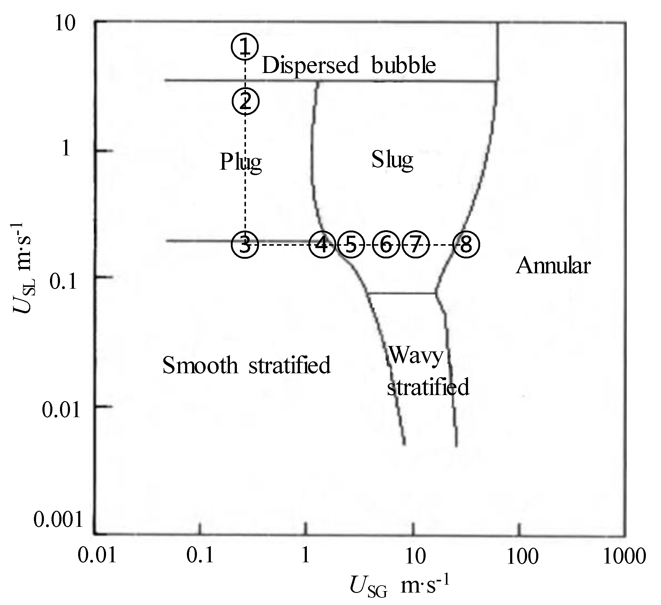
2.3. Physical Parameter Range

The physical parameters of the oil and natural gas used in our calculations are listed in

Table 1. The physical properties of oil and natural gas at 4 MPa and 20 °C.

Working Fluid	Viscosity/m2·s−1	Density/kg·m−3
Oil	3.79 × 10−5	845
Natural gas	1.38 × 10−6	8.7

, which are reliable ones according to the literature (Khaledi [1]), at 20 °C temperature and 4 MPa pressure of the horizontal pipeline of oil-and-gas mixing. In order to evaluate the versatility of the algorithm and satisfy all flow types as much as possible, eight working cases with different inlet flow rates were considered, and the ranges of gas and oil superficial velocities are shown in

Table 2. Flow parameters of oil and gas.

Case No.	Inlet Velocity/m·s−1		Superficial Velocity/m·s−1
	Oil	Gas	Oil	Gas
1	28.88	1.42	5.53	0.14
2	5.78	1.42	1.11	0.14
3	0.87	1.42	0.17	0.14
4	0.87	14.15	0.17	1.38
5	0.87	28.31	0.17	2.77
6	0.87	56.62	0.17	5.53
7	0.87	99.08	0.17	9.68
8	0.87	283.09	0.17	27.65

. The superficial velocity is the average speed at which the gas phase and the liquid phase flow through the whole cross-section of the pipeline independently, which is commonly used as a key parameter for distinguishing between different flow patterns in two-phase flow. The superficial velocity of natural gas U_SG and the superficial velocity of the oil U_SL are

$$U_{\mathrm{SG}}={\displaystyle \frac{u_{\mathrm{in},\mathrm{g}}\mathsf{\pi }{R}_{\mathrm{in},\mathrm{g}}^2}{\mathsf{\pi }{R}_{\mathrm{test}}^2}}$$

(17)

$$U_{\mathrm{SL}}={\displaystyle \frac{u_{\mathrm{in},l}\mathsf{\pi }{R}_{\mathrm{in},l}^2}{\mathsf{\pi }{R}_{\mathrm{test}}^2}}$$

(18)

where u_in,g and u_in,l are the inlet velocities of the gas and oil, m·s⁻¹, respectively. The R_in and R_test are the inlet radius and stabilized segment radius of the mixer, m, respectively.

In Figure 3, the working cases simultaneously defined by the U_SL and U_SG are marked in the Mandhane flow regime map [14], which is the most widely used flow regime boundary map for gas–liquid two-phase flow.

2.4. Mesh Independence Verification and Validation Test

A grid-independent experiment was conducted to calculate the liquid film thickness after flow stabilization for Case 8 at varying grid resolutions. The results are presented in

Table 3. Grid independence tests.

Elements No.	68,965	108,637	155,594	192,094
Film thickness/mm	7.68	7.96	8.16	8.16

. It was observed that the liquid film thickness remained relatively unchanged once the number of cells reached or exceeded 155,594. Therefore, a grid resolution of 155,594 was adopted for subsequent calculations.

To validate the calculation model, predictive computations were performed using the same pipeline structure and flow data from the literature (Feng and Wang [35]), and the results were compared with experimental data. The horizontal pipeline of oil-and-gas mixed transportation was 0.253 m. The superficial velocity of the gas was 1.27 m·s⁻¹, while the superficial velocity of the oil was 0.16 m·s⁻¹. As shown in Figure 4, the predictive flow regime corresponded to a slug flow, corresponding to the available literature.

Furthermore, as shown in

Table 4. The comparisons of flow regimes obtained from the OpenFOAM calculation results with the Brill and Mandhane discriminant methods.

Case No.	USL/m·s−1	USG/m·s−1	OpenFOAM	Bill	Mandhane
1	5.53	0.14	Bubble	Bubble	Dispersed bubble
2	1.11	0.14	Bubble	Bubble	Plug
3	0.17	0.14	Plug	Stratified	Plug / Stratified *
4	0.17	1.38	Slug	Slug	Plug / Slug / Stratified *
5	0.17	2.77	Annular	Slug	Slug
6	0.17	5.53	Annular	Slug	Slug
7	0.17	9.68	Annular	Annular/Slug	Slug
8	0.17	27.65	Annular	Annular	Annular

* / means that, according to the algorithm’s calculation results, the flow state is at an intersection. U_SL is the superficial velocity of the oil, and the U_SG is the superficial velocity of the natural gas.

, the simulation results of eight cases with the OpenFOAM algorithms in this study were compared with predictions using the Brill and Mandhane flow regime identification criteria under the same operating cases, respectively.

After employing the mixer, the oil phase was injected from the boundary of the gas phase. Correspondingly, the oil–gas two-phase flow mainly tended to be an annular flow, not a stratified flow. Moreover, neither the Brill criteria nor the Mandhane criteria considered the oil’s physical property of high viscosity, which caused the gas–liquid interface to be smoother and closer to the upper and lower liquid levels. Therefore, there was a subtle difference in Case 5, which showed an incomplete annular flow sooner than other cases. Nevertheless, the overall transformation boundary between the different flow regimes roughly satisfied the laws of the Brill criteria.

3. Results and Discussion

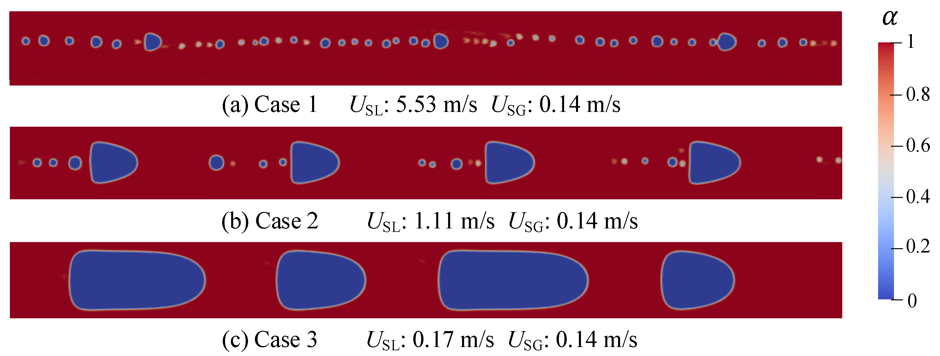
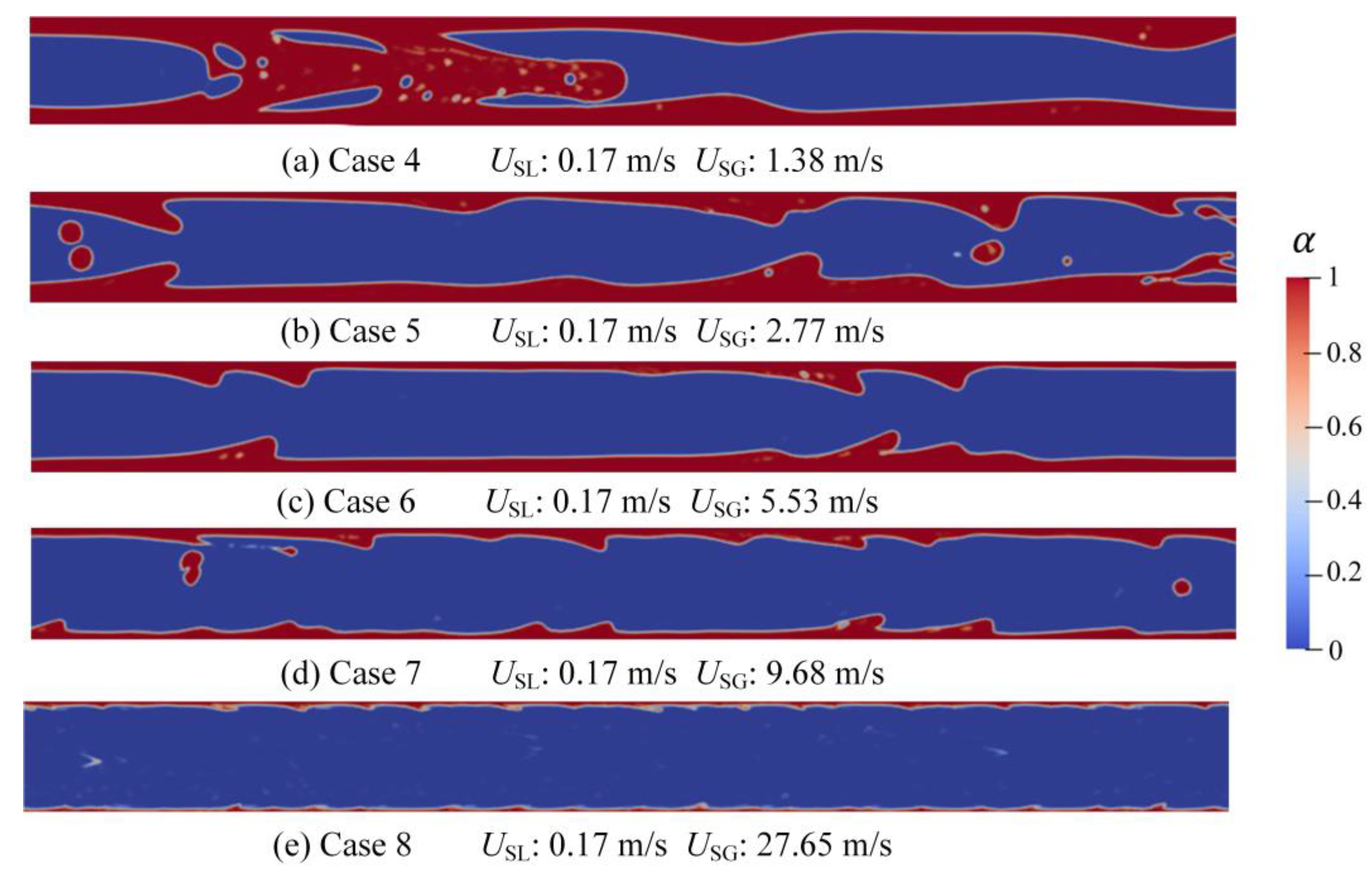
3.1. Bubble Flow and Plug Flow

For Cases 1~3, the superficial velocity of natural gas was constant at 0.138 m/s, while that of oil was variable. The diversity in the gas–liquid two-phase flow regime could be clearly observed, as shown in Figure 5.

In Case 1, as shown in Figure 5a, the flow rate of the liquid phase was much larger than that of the gas phase, with a 0.98 of void fraction at the inlet. Under this circumstance, the natural gas was entrained by the larger liquid flow rate at the center of the pipeline and dispersed into a series of small rectilinear bubbles around its centerline. As the liquid phase decreased, in Case 2, as shown in Figure 5b, the volume fraction at the inlet was 0.89, and the small bubbles formed in the pipeline gradually merged into large bubbles, which were characterized by a sharper head and a flatter tail and tailed by a cluster of small bubbles. In general, the gas–liquid two-phase flow was still stable. As shown in Figure 5c, in Case 3, the flow rate of oil was further decreased, and the volume fraction at the inlet was lowered to a value of 0.55. Correspondingly, a very clear plug flow was manifesting as larger bullet-shaped bubbles, almost occupying the entire pipe cross-section with tailed small bubbles disappearing. Meanwhile, another prominent feature concerned plug-shaped large and small bubbles, also called gas plugs, appearing intermittently, which might have been due to pressure fluctuations.

To further investigate the formation of bubbles, the gas-phase and liquid-phase velocity profiles in and around the plug bubbles are depicted in Figure 6 for Cases 2 and 3, respectively, where the black solid lines denote the outlines of the bubbles and the black dash lines denote the contour velocities of the gas phase and the liquid phase. It is apparent that the velocity isolines in the bubble heads are dome-shaped, while the ones in their tails are horseshoe-shaped. As shown in Figure 6a for Case 2, the annular liquid film around the bubble, due to the low velocity relative to the large bubble, slipped down from the tail of the bubble and was squeezed into the wake area. The vortex from the wake effect pushed the liquid downstream to move forward at a higher speed, tearing the bubble tail into small bubbles. However, due to the high viscosity of the oil, the generated small bubbles in the wake were not very broken compared to the air–water two-phase flow. As shown in Figure 6b, the bubbles in Case 3 further merged to form a larger bubble, also called Taylor bubble. The flow regime was determined to be slug flow. When the flow rate of the bubble decreased, the stirring effect in the wake decreased, and small bubbles were no longer formed, developing into other large bubbles.

Due to the difference in density and viscosity between bubbles and liquids, bubbles were affected by forces such as friction force and body force in the flow field, resulting in a substantial difference in the velocity between bubbles and fluids, that is, the slip velocity, which reflected the motion state of bubbles and liquid, related to the diameter and flow velocity of the bubble. The slip velocity was defined as u_gl:

$$u_{\mathrm{gl}}=u_{\mathrm{g}}-u_l$$

(19)

where u_g is the gas velocity, and u_l is the oil velocity.

Figure 7 depicts the fluid velocity and volume of fraction along the diameter of the cross-sections of gas slug in Cases 2 and 3, respectively.

Table 5. The gas thickness H, fluid velocity u_l, and slip velocity u_gl at the gas–liquid interface under two cases.

Case No.	H/mm	ul/m·s−1	ugl/m·s−1
2	42	2.66	0.038
3	61	0.05	0.057

lists the gas slug thickness (that is, the length of the bubble along the diameter direction), the fluid velocity, and the slip velocity at the gas–liquid interface for two cases.

From Figure 7, it can be seen that the volume fraction has a noticeable 0–1 boundary, which is the gas–liquid interface. Along the diameter direction, the flow velocity is high in the pipe centerline and low at both pipe walls. At the same time, the closer a bubble is to the center of the pipe, the greater the velocity of the bubble, that is, the velocity of the central gas slug is greater than the velocity of the liquid.

Combining Figure 7 and Table 5, it is worth noting that, compared with Case 3, the liquid velocity in Case 2 was larger, and the gas thickness H was smaller, while the slip velocity was larger. The reason for this was that the gas content of the two-phase flow in Case 2 was very small, and the entrainment effect of the liquid played a crucial role, which promoted the forward movement and coalescence of the gas. In Case 3, the volume fraction at the inlet was 0.55, which increased the viscous influence between the gas and the liquid. Coupled with the decrease in the liquid speed, the slip velocity at the gas–liquid interface was small, resulting in a larger shape of the bubbles and a more stable flow.

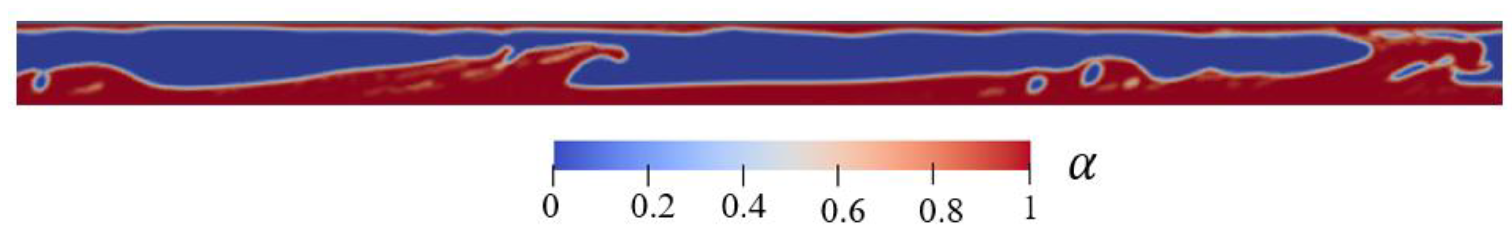
3.2. Slug Flow and Wave Flow

In order to reveal the effect of gas flow variation on the flow regime, the superficial velocity of oil was kept at 0.166 m/s, and the superficial velocity of gas was varied. The flow regime distribution of Cases 4~8 is obtained from Figure 8.

As shown in Figure 8a, with the increase in gas velocity, the gas slugs were connected to each other. The faster gas flow blew through the liquid film, creating a gas column. The liquids on the upper and lower walls were intermittently connected, resulting in large pressure fluctuations, which posed a greater threat to the safety of the pipeline. This kind of working condition should be avoided as much as possible in actual pipeline transportation. With the further increase in the gas velocity, the liquid film on the upper and lower walls gradually became thinner, showing a clear annular flow. When the gas velocity was high, the phenomenon of oil rolling up and being carried in the gas flow could be seen. Compared to the commonly observed stratified wave flow in horizontal pipelines, this study demonstrated a greater occurrence of annular flow. The impact of gravitational convection was not significant. This could be attributed to the use of a special mixer with a symmetrical structure, as well as the fact that, at high gas flow rates, the gas accumulated at the pipe center while the liquid formed a thin film along the pipe wall, which aligned with the findings in Reference [36].

Variations in the pressure over time at the pipeline cross-section, 2540 mm away from the entrance, in Case 4 and Case 5 were calculated, and the result is shown in Figure 9. The pressure difference is expressed as the pressure minus the minimum pressure within the time period, which evidently corresponds to the fluctuation in pressure. It can be noted that there was a large pressure peak in Case 4. The reason was that, at that moment, the test cross-section was completely blocked by the oil (as shown in Figure 9a–c), while at other times, the flow in the pipeline was very stable due to the low gas–liquid flow rate (as shown in Figure 9d). In Case 5, due to the lower volume fraction, the pipeline did not appear blocked, that is, there was no very large pressure peak. However, the liquid film was set off by the rapid-passing airflow, and there were still more frequent but small pressure fluctuations. Therefore, slug flow should be avoided in real production, while annular flow has better performance in terms of pressure fluctuation because of the noticeable drag reduction effect.

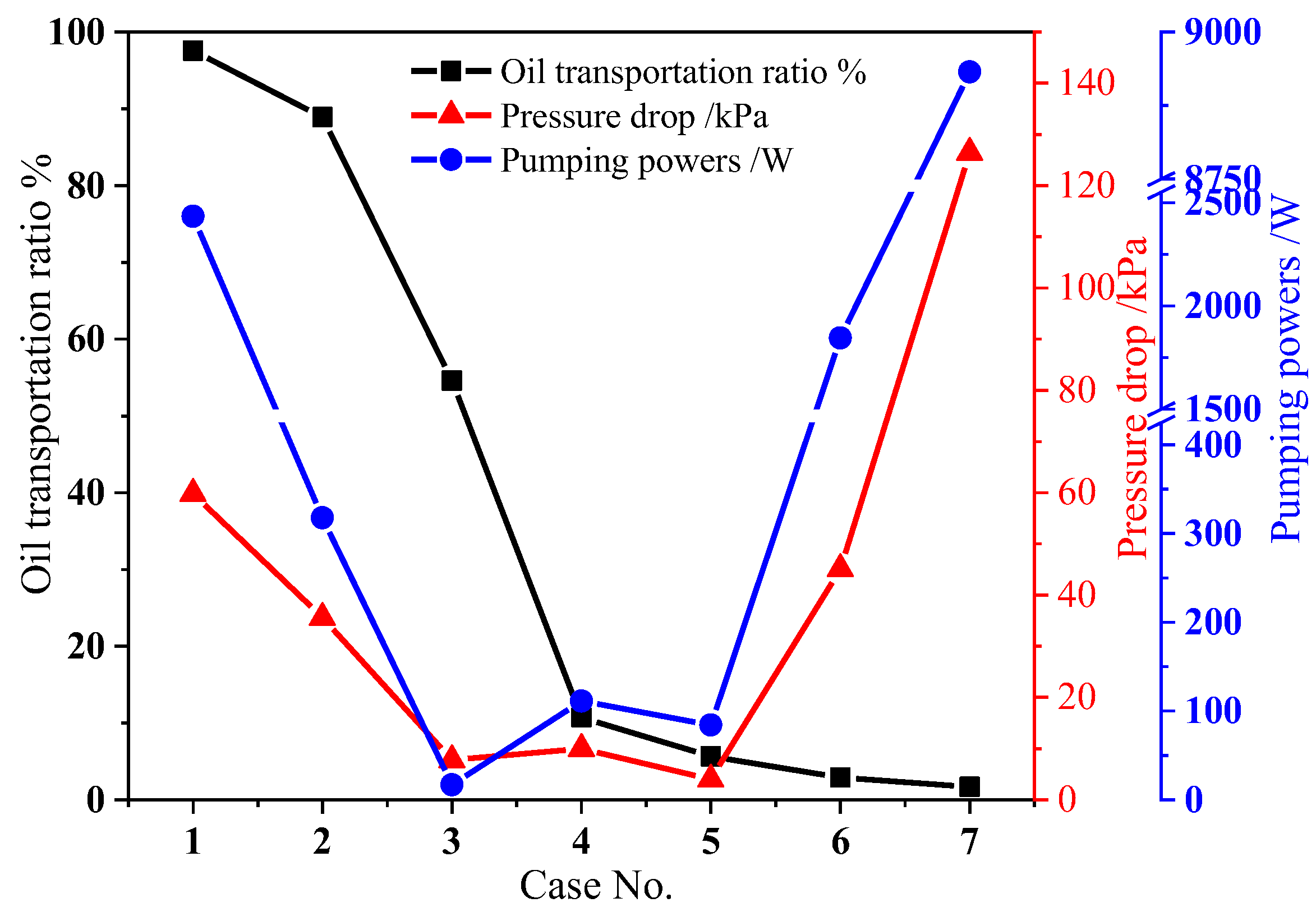
3.3. Energy Consumption Analysis

The best working condition meeting the lowest pump power loss and the highest oil transportation ratio was revealed, on the basis of safe transportation. The oil transportation ratio was defined as the proportion of the oil transportation content in the total fluid, meaning that the greater the oil superficial velocity relative to that of gas, the greater the oil transportation ratio:

$$\varphi ={\displaystyle \frac{U_{SL}}{U_{SL}+U_{SG}}}$$

(20)

It was clear that, in Case 1, the oil transportation ratio was the greatest, followed by Cases 2~8. However, the large flow rate caused more pump power to be required. The pumping power P_pump was defined as follows:

$$P_{\mathrm{pump}}={\displaystyle \frac{Q\Delta P}{{\eta }_{\mathrm{pump}}}}$$

(21)

where Q is the volumetric flow of the oil–natural gas mixture; ΔP is the maximum pressure difference between import and export in two-phase transportation; and η_pump is the pump efficiency, corresponding to 70% in our study.

Figure 10 illustrates the oil transport rate, pressure drop, and pump power consumption under operating Cases 1 through 7. It is evident that the pump power loss was minimal in Cases 3 to 5. Among these, Case 4, representing slug flow, was prone to intermittent blockages, which caused abrupt pressure fluctuations and undermined system stability. In contrast, Case 5, which corresponded to a stable annular flow, resulted in the least pressure drop loss and was an ideal condition for oil–gas multiphase transport. However, its oil transport rate was relatively low. Additionally, Case 3, characterized by stable plug flow, offered the advantages of a high oil transport rate and low pump power consumption, making it another recommended operational condition. Noteworthily, the ratio of oil and gas needed to be strictly controlled to prevent discontinuous slug flow if the amount of oil was too small.

4. Conclusions

To promote the transportation performance of gas and oil systems, the flow management of high-viscosity crude oil and natural gas after passing through a mixer commonly adopted in gas-and-oil-gathering systems was analyzed using the OpenFOAM software. The flow regimes were essentially consistent with other flow regime identification methods (Brill criterion and Mandhane criterion). The main conclusions were the following:

(a)

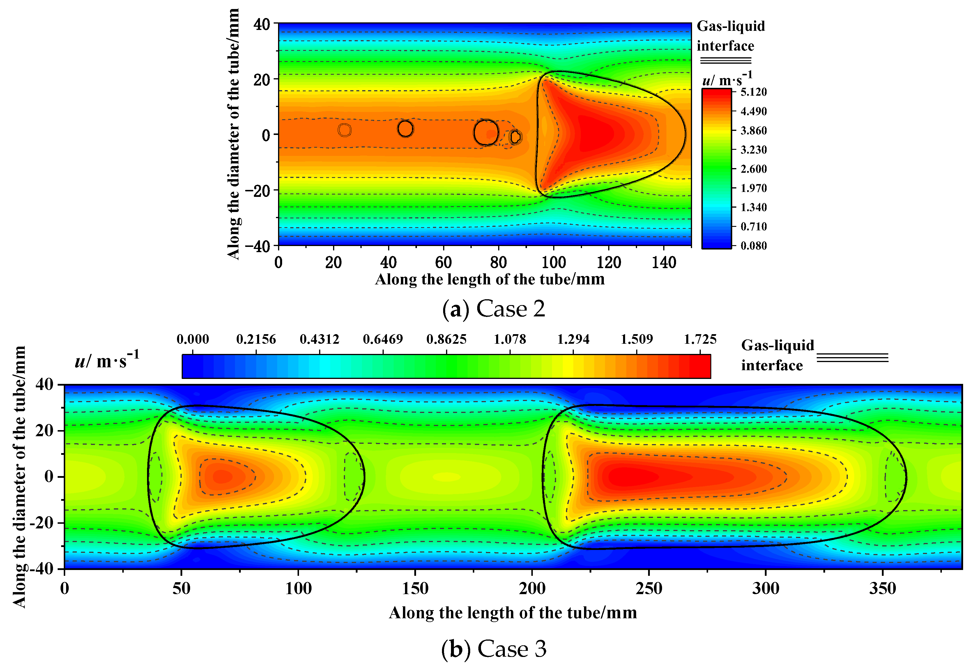
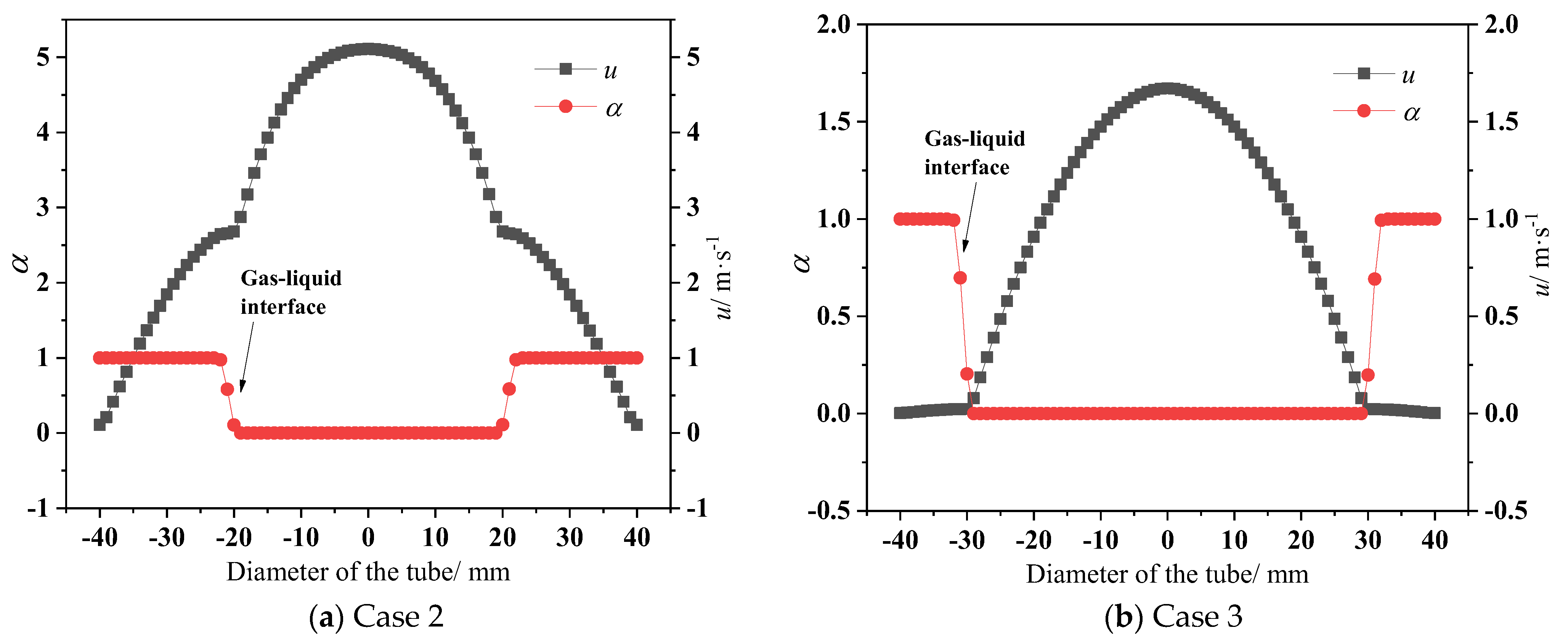
The growth of bubbles within the pipeline was influenced by the interplay of volume fraction, flow velocity, and bubble slip velocity.

(b)

In the plug flow, owing to the high viscosity of the oil, the small bubbles formed in the wake remained largely intact, in contrast to the fragmentation seen in air–water two-phase flows.

(c)

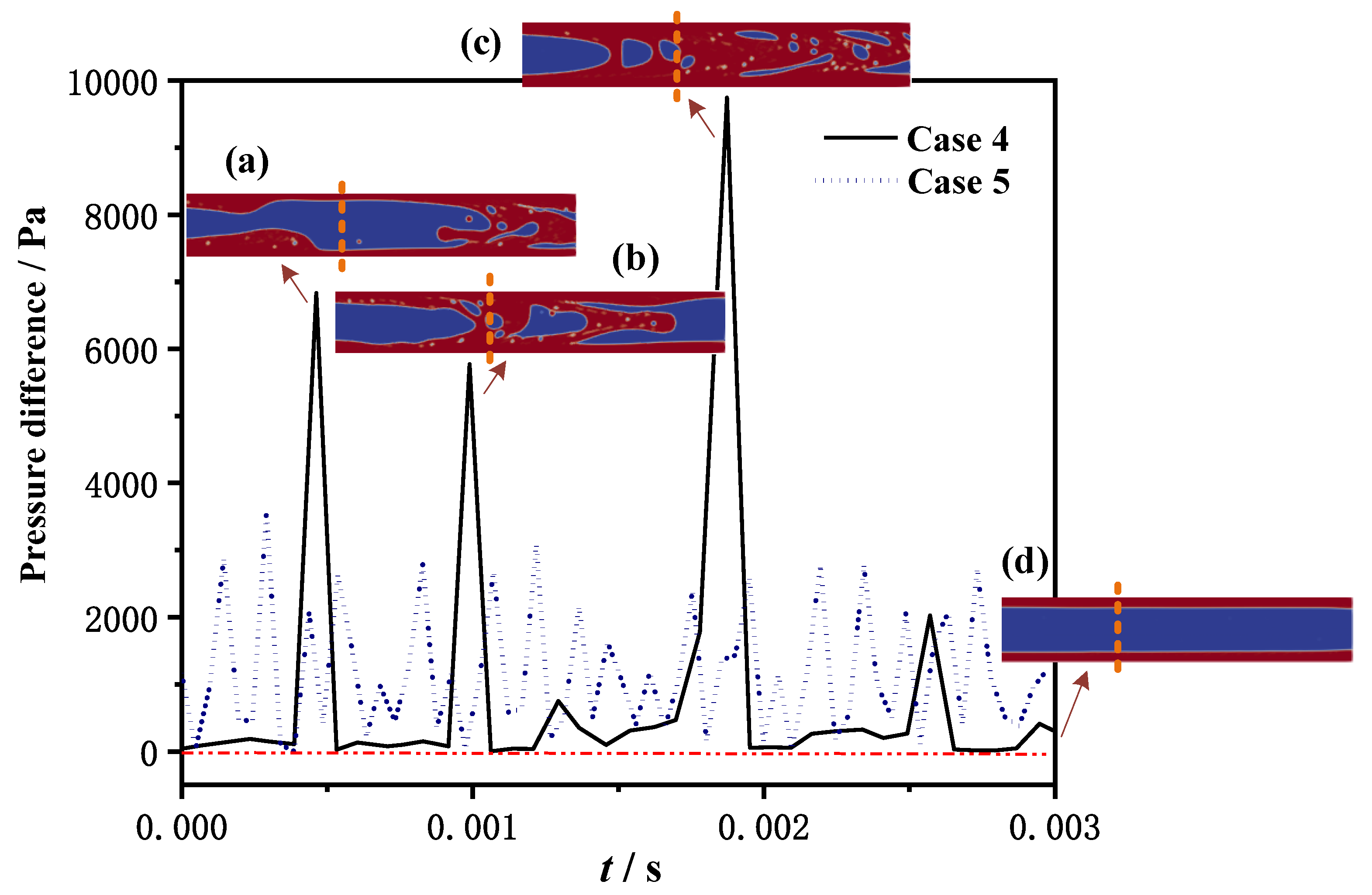
In the slug flow, the intermittent interaction of liquid with the upper and lower walls resulted in significant pressure fluctuations. This phenomenon should be avoided in practical operations.

(d)

The stable annular flow exhibited the lowest pressure drop loss, making it the ideal condition for oil–gas multiphase transport. The plug flow, on the other hand, offered the advantages of high oil transportation rates and low pump power consumption.

5. Future Perspectives

(a) Regarding computational constraints and flow regime selection, due to limitations in computational resources, this study focused on a few typical flow regimes (bubble flow, plug flow, slug flow, wavy flow, and annular flow), selected based on the Mandhane flow regime map. However, a more comprehensive set of flow regimes was not considered due to the computational workload. In future studies, it is recommended to expand the range of experimental conditions to include a broader array of flow regimes, which would enhance the generalizability of the findings.

(b) Regarding viscosity range and comparative analysis, this study exclusively examined a single high-viscosity fluid for the simulations. Given the diverse viscosities found in actual oil reservoirs, future research should incorporate a range of viscosities corresponding to different types of heavy oils encountered in field operations. A comparative study of these fluids would provide a more comprehensive understanding of their behavior under varying flow conditions and contribute to the development of more robust predictive models for industrial applications.

References

1. Khaledi, H.A.; Smith, I.E.; Unander, T.E.; Nossen, J. Investigation of two-phase flow pattern, liquid holdup and pressure drop in viscous oil–gas flow. Int. J. Multiph. Flow 2014, 67, 37–51. [Google Scholar] [CrossRef]
2. Otsubo, Y. Hydrogen compression and long-distance transportation: Emerging technologies and applications in the oil and gas industry—A technical review. Energy Convers. Manag. X 2025, 25, 100836. [Google Scholar] [CrossRef]
3. Jansen, F.E.; Shoham, O.; Taitel, Y. The elimination of severe slugging—Experiments and modeling. Int. J. Multiph. Flow 1996, 22, 1055–1072. [Google Scholar] [CrossRef]
4. Baliño, J.L.; Burr, K.P.; Nemoto, R.H. Modeling and simulation of severe slugging in air–water pipeline–riser systems. Int. J. Multiph. Flow 2010, 36, 643–660. [Google Scholar] [CrossRef]
5. Yu, H.; Xu, Q.; Cao, Y.; Huang, B.; Guo, L. Effects of riser height and pipeline length on the transition boundary and frequency of severe slugging in offshore pipelines. Ocean Eng. 2024, 298, 117253. [Google Scholar] [CrossRef]
6. Zhao, X.; Xu, Q.; Fu, J.; Chang, Y.; Wu, Q.; Guo, L. Study on eliminating severe slugging by manual and automatic choking in long pipeline-riser system. Chem. Eng. Sci. 2024, 292, 119978. [Google Scholar] [CrossRef]
7. Baba, Y.D.; Aliyu, A.M.; Archibong, A.E.; Abdulkadir, M.; Lao, L.; Yeung, H. Slug length for high viscosity oil-gas flow in horizontal pipes: Experiments and prediction. J. Pet. Sci. Eng. 2018, 165, 397–411. [Google Scholar] [CrossRef]
8. Liu, X.-M.; Zhong, H.-Q.; Li, Y.-C.; Liu, Z.-N.; Wang, Q. Experimental study of flow patterns and pressure drops of heavy oil-water-gas vertical flow. J. Hydrodyn. Ser. B 2014, 26, 646–653. [Google Scholar] [CrossRef]
9. Chen, K.; Wang, X.; Peng, H.; Liu, W.; Chen, P.; Wen, L. Study on water fraction of oil–gas–water three-phase flow based on electrical methods. Energy Rep. 2022, 8, 90–98. [Google Scholar] [CrossRef]
10. Wang, D.; Jin, N.; Zhai, L.; Ren, Y. Quantitative research of the liquid film characteristics in upward vertical gas, oil and water flows. Chin. J. Chem. Eng. 2023, 54, 67–79. [Google Scholar] [CrossRef]
11. Chang, Y.; Xu, Q.; Zou, S.; Zhao, X.; Wu, Q.; Wang, Y.; Thévenin, D.; Guo, L. Experiments and predictions for severe slugging of gas-liquid two-phase flows in a long-distance pipeline-riser system. Ocean Eng. 2024, 301, 117636. [Google Scholar] [CrossRef]
12. Li, Z.; Tan, C.; Zhang, S.; Dong, F. Global-local state analysis and monitoring-based velocity measurement of oil–gas–water three-phase flow. Chem. Eng. J. 2024, 497, 154759. [Google Scholar] [CrossRef]
13. Abdelsamie, A.; Voß, S.; Berg, P.; Chi, C.; Arens, C.; Thévenin, D.; Janiga, G. Comparing LES and URANS results with a reference DNS of the transitional airflow in a patient-specific larynx geometry during exhalation. Comput. Fluids 2023, 255, 105819. [Google Scholar] [CrossRef]
14. Mandhane, J.M.; Gregory, G.A.; Aziz, K. A flow pattern map for gas—Liquid flow in horizontal pipes. Int. J. Multiph. Flow 1974, 1, 537–553. [Google Scholar] [CrossRef]
15. Mukherjee, H.; Brill, J.P. Empirical equations to predict flow patterns in two-phase inclined flow. Int. J. Multiph. Flow 1985, 11, 299–315. [Google Scholar] [CrossRef]
16. Taitel, Y.; Dukler, A.E. A model for predicting flow regime transitions in horizontal and near horizontal gas-liquid flow. AIChE J. 1976, 22, 47–55. [Google Scholar] [CrossRef]
17. Taitel, Y.; Dukler, A.E. A model for slug frequency during gas-liquid flow in horizontal and near horizontal pipes. Int. J. Multiph. Flow 1977, 3, 585–596. [Google Scholar] [CrossRef]
18. Lin, P.Y.; Hanratty, T.J. Prediction of the initiation of slugs with linear stability theory. Int. J. Multiph. Flow 1986, 12, 79–98. [Google Scholar] [CrossRef]
19. Shaaban, O.M.; Al-Safran, E.M. Prediction of slug length for high-viscosity oil in gas/liquid horizontal and slightly inclined pipe flows. Geoenergy Sci. Eng. 2023, 221, 211348. [Google Scholar] [CrossRef]
20. Padoin, N.; Souza, A.Z.D.; Ropelato, K.; Soares, C. Numerical simulation of isothermal gas−liquid flow patterns in microchannels with varying wettability. Chem. Eng. Res. Des. 2016, 109, 698–706. [Google Scholar] [CrossRef]
21. Yan, K.; Che, D. A coupled model for simulation of the gas–liquid two-phase flow with complex flow patterns. Int. J. Multiph. Flow 2010, 36, 333–348. [Google Scholar] [CrossRef]
22. Nieves-Remacha, M.J.; Yang, L.; Jensen, K.F. OpenFOAM Computational Fluid Dynamic Simulations of Two-Phase Flow and Mass Transfer in an Advanced-Flow Reactor. Ind. Eng. Chem. Res. 2015, 54, 6649–6659. [Google Scholar] [CrossRef]
23. Nagarajan, H.K.; Trujillo, M.F. Quantifying a common inconsistency in RANS-VoF modeling of water and oil core annular flow. Int. J. Multiph. Flow 2024, 181, 105008. [Google Scholar] [CrossRef]
24. Li, H.; Pourquié, M.J.B.M.; Ooms, G.; Henkes, R.A.W.M. DNS and RANS for core-annular flow with a turbulent annulus. Int. J. Multiph. Flow 2024, 174, 104733. [Google Scholar] [CrossRef]
25. Li, S.; Kang, Y.; Wang, T.; Pan, W.; Li, C.X. Numerical Simulation on Jet Flow Characteristics of Pressure Drop Sleeve of Drain Regulating Valve. Fluid Mach. 2019, 47, 19–26. [Google Scholar] [CrossRef]
26. Warren, B.A.; Klausner, J.F. Developing Lengths in Horizontal Two-Phase Bubbly Flow. J. Fluids Eng. 1995, 117, 512–518. [Google Scholar] [CrossRef]
27. Salcudean, M.; Groeneveld, D.C.; Leung, L. Effect of flow-obstruction geometry on pressure drops in horizontal air-water flow. Int. J. Multiph. Flow 1983, 9, 73–85. [Google Scholar] [CrossRef]
28. Hirt, C.W.; Nichols, B.D. Volume of fluid (VOF) method for the dynamics of free boundaries. J. Comput. Phys. 1981, 39, 201–225. [Google Scholar] [CrossRef]
29. Brackbill, J.U.; Kothe, D.B.; Zemach, C. A continuum method for modeling surface tension. J. Comput. Phys. 1992, 100, 335–354. [Google Scholar] [CrossRef]
30. Bankoff, S.G.; Lee, S.C. A Comparison of Flooding Models for Air-Water and Steam-Water Flow. In Advances in Two-Phase Flow and Heat Transfer; Kakaç, S., Ishii, M., Eds.; NATO ASI Series; Springer: Dordrecht, The Netherlands, 1983; Volume 64, pp. 745–780. [Google Scholar] [CrossRef]
31. Weller, H.G. A New Approach to VOF-based Interface Capturing Methods for Incompressible and Compressible Flow. Tech. Rep. 2008, 4, 35. [Google Scholar]
32. Launder, B.E.; Sharma, B.I. Application of the energy-dissipation model of turbulence to the calculation of flow near a spinning disc. Lett. Heat Mass Transf. 1974, 1, 131–137. [Google Scholar] [CrossRef]
33. Li, H.; Pourquié, M.J.B.M.; Ooms, G.; Henkes, R.A.W.M. Simulation of vertical core-annular flow with a turbulent annulus. Int. J. Multiph. Flow 2023, 167, 104551. [Google Scholar] [CrossRef]
34. Li, H.; Pourquié, M.J.B.M.; Ooms, G.; Henkes, R.A.W.M. Simulation of a turbulent annulus with interfacial waves in core-annular pipe flow. Int. J. Multiph. Flow 2022, 154, 104152. [Google Scholar] [CrossRef]
35. Feng, G.K.; Wang, X. Oil & Gas Gathering & Transportation; University of Petroleum Press: Dongying, China, 1988; pp. 154–159. [Google Scholar]
36. Alameedy, U.; Al-Sarkhi, A.; Abdul-Majeed, G. Comprehensive review of severe slugging phenomena and innovative mitigation techniques in oil and gas systems. Chem. Eng. Res. Des. 2025, 213, 78–94. [Google Scholar] [CrossRef]
Figure 1. A sketch diagram of flowline in an oil-and-gas-gathering system.
Energies 18 01550 g001
Figure 2. The model of the oil and gas mixer.
Energies 18 01550 g002
Figure 3. The working points of eight cases 1–8 in the Mandhane flow regime map. USL is the superficial velocity of the oil, and the USG is the superficial velocity of the natural gas.
Energies 18 01550 g003
Figure 4. Simulation results obtained using the OpenFOAM software with example data in the literature [35]. α represents the volume fraction of oil; the distribution of oil and gas is shown in red and blue, respectively.
Energies 18 01550 g004
Figure 5. Calculation results of gas–liquid two-phase flow regime for Cases 1~3. α represents the volume fraction of oil; the distribution of oil and gas is shown in red and blue, respectively.
Energies 18 01550 g005
Figure 6. Gas–liquid velocity distribution in Cases 2 and 3. The black solid lines denote the outlines of the bubbles. The black dash lines denote the contour velocities of the gas phase and the liquid phase.
Energies 18 01550 g006
Figure 7. The flow velocity (u) and volume of fraction (α) along the diameter of Cases 2 and 3.
Energies 18 01550 g007
Figure 8. Calculation results of gas–liquid two-phase flow regime for Cases 4~8. α represents the volume fraction of oil; the distribution of oil and gas is shown in red and blue, respectively.
Energies 18 01550 g008
Figure 9. The pressure changes in Case 4 and Case 5 at the 2540 mm mark in the pipeline cross-section over time. The small pictures (ad) show the distribution of flow regimes in different states, and the yellow dotted line indicates the position of the 2540 mm mark in the cross-section.
Energies 18 01550 g009
Figure 10. The oil transport rate, pressure drop, and pumping power consumption under operating Cases 1 through 7.
Energies 18 01550 g010