Article

A Method for the Modular Power Flow Analysis of Extensive Distribution Grids

by
Daniel-Leon Schultis
1,2,* and
Clemens Korner
1
1
AIT Austrian Institute of Technology GmbH, Giefinggasse 4, 1210 Vienna, Austria
2
Magnus Energy B.V., Gooimeer 5-39, 1411 DD Naarden, The Netherlands
*
Author to whom correspondence should be addressed.
Energies 2025, 18(6), 1559; https://doi.org/10.3390/en18061559
Submission received: 11 February 2025 / Revised: 5 March 2025 / Accepted: 19 March 2025 / Published: 20 March 2025
(This article belongs to the Section F1: Electrical Power System)

Abstract

:
The widespread deployment of distributed energy resources including volatile renewable generation raises the need for detailed distribution network analysis. In many cases, the vast system sizes make the joint analysis of multiple voltage levels computationally impracticable. Consequently, most studies focus on single or selected voltage levels and represent subordinate system portions by conventional static load models. Their parameters are usually identified by simplified aggregation methods that do not consider the effects of the network, i.e., network losses and spatial voltage variations. This approach involves inaccuracies and does not allow for validating compliance with the voltage and current limits inside subordinate system parts that are not explicitly represented in the model. In response to this challenge, this paper extends the static load model by including new parameters, i.e., the boundary voltage limits, and describes the associated component-based parameter identification method. Their combination paves the way for a modular power flow approach, which supports the separate investigation of different system portions without introducing considerable inaccuracies, enabling the systematic, precise, and computationally practicable power flow analysis and validation of voltage and current limit compliance in large distribution systems. The proposed concepts are applied to a synthetic distribution system to facilitate their use and showcase their usefulness.

1. Introduction

Power flow analysis is essential for power system planning and operation, as it allows for validating compliance with the operational network limits, determining losses, and calculating the power transfers between different networks. Furthermore, it constitutes the basis for subsequent analyses such as reliability, power quality, and transients [1].
Precise static models of all relevant system components are necessary to obtain meaningful power flow results [2]. While sufficient models exist for individual network components such as lines, transformers, and reactive power devices, load modeling still presents a challenging task as (bus) loads may include numerous elements with time- and weather-dependent characteristics and complex interdependencies, such as lines, shunt capacitors, electric vehicles, distributed generators, household devices, and on-load tap changers (OLTCs) [3]. Various static load models are currently available, including linear, exponential, polynomial, comprehensive, and power electronic-interfaced ones, as well as the static induction motor model [4]. They generally describe the active and reactive power contributions of a PQ-node element by assuming an instantaneous response to voltage magnitude and frequency deviations [see Equation (1)].
P = H P V , f = P n · h P V , f
Q = H Q V , f = Q n · h Q V , f
h P V n , f n = h Q V n , f n = 1
where H P , H Q , h P , and h Q are functions; V n and f n are the nominal voltage magnitude and frequency; V and f are the actual voltage magnitude and frequency; P n and Q n are the load’s active and reactive power contributions based on the nominal voltage magnitude and frequency; and P and Q are the load’s active and reactive power contributions based on the actual voltage magnitude and frequency. Although the effects of frequency deviations could be captured by the available load models, they are commonly neglected in power flow analysis [5], yielding the model structure given in Equation (2).
P = H P V = P n · h P V
Q = H Q V = Q n · h Q V
h P V n = h Q V n = 1
Both the active and reactive power contributions at nominal voltage and the associated voltage dependency terms exhibit temporal variations. The variability in the former is attributed to weather-dependent injections from renewable energy sources and the stochastic activation and deactivation of load devices. Meanwhile, the fluctuations in the latter are a consequence of the varying load composition and spatial voltage variations within the distribution network. Spatial voltage variations are crucial for the aggregation of voltage-dependent loads: In a distribution network, all loads (including distributed generation) face different voltages and thus lie—with respect to an instance of time—on different operating points of their P(V) and Q(V) characteristics. Consequently, the aggregate characteristics differ from the sums of the individual ones, even if network losses are neglected. Reference [6] analyzes this effect and observes that by neglecting spatial voltage variations, substantial inaccuracies are introduced, particularly when the aggregated loads possess intense voltage dependencies, such as Volt/var-controlled photovoltaic (PV) inverters.
In general, measurement- and component-based approaches, or any combination of them, are used to identify the parameters of the available static load models to approximate the aggregate load-voltage dependency at specific system buses [7]. Measurement-based approaches leverage measurement data and computation techniques such as statistics, artificial intelligence, and pattern recognition to determine the load model parameters for a specific network node. These approaches lack generalizability as the measurements are recorded in certain time periods at specific locations [3]. As the measurement data contain information about the load composition and the subordinate network, they offer the possibility to determine accurate time-variant load model parameters. Such parameters are calculated, for instance, by the methods presented in [8,9] for polynomial and static induction motor models.
Component-based methods determine the load model parameters at a specific network node by aggregating the individual models of the subordinate components. Most approaches neglect network losses and spatial voltage variations to obviate the need for detailed network modeling [see Equations (A1)–(A5) in the Appendix A for more details]. References [10,11,12,13,14,15] calculate aggregate static load models for residential dwellings, low voltage networks, and entire distribution networks, without considering the networks’ impact on the resulting load characteristics (dwellings also have an internal network). A synthesis load model, which connects various load models through one common impedance, denoted as equivalent distribution network impedance, is presented in [16], and possible parameter identification methods are discussed in [17,18]. This common impedance enables the simplified consideration of distribution network losses; however, all load components have the same terminal voltage, thus neglecting spatial voltage variability. Contrarily, reference [19] introduces a bottom-up procedure for the systematic incorporation of distribution network impedances into a reduced form of the composite load model that consists of a constant impedance and induction motor load. The resulting model considers spatial voltage variability, but the underlying aggregation method lacks the possibility to consider other load models (e.g., linear, exponential, and polynomial) as well as local inverter controls such as Volt/var and Volt/Watt, which usually have piecewise linear characteristics. The current state-of-the-art does not offer a universally applicable method for the accurate aggregation of voltage-dependent loads that considers the effects of the intermediate network, i.e., network losses and spatial voltage variations.
However, power flow analysis is traditionally applied to transmission grids, and the connected distribution systems are represented by lumped models. The distribution grids were sufficiently dimensioned based on the estimated peak power demand and the expected annual energy demand increase to obviate the need for detailed system analysis. The continuously progressing deployment of distributed energy resources and sophisticated smart grid applications, such as demand response and Volt/var optimization, raise the need for detailed distribution system analysis [20]. Distribution networks can have many more nodes than transmission grids and often consist of ramified structures with thousands of nodes and branches that interconnect immense numbers of customer plants (CPs). Most European distribution systems encompass the high (HV), medium (MV), and low voltage (LV) levels [21]. Their vast sizes make the joint simulation of multiple system levels highly computation- and memory-intensive and, in many cases, impracticable. For that reason, many studies focus on a single or selected voltage levels and use static load models according to Equation (2) for the adjacent system parts that are not the subject of investigation, e.g., [22,23,24].
Additionally, distribution networks are generally subject to thermal and voltage limits. Thermal limits are technical limitations that ensure the durability of the electrical equipment and are usually considered as static current constraints. In contrast, voltage limits are stipulated by standards to guarantee a certain quality of supply at the delivery points (DPs) of grid customers. For instance, the European standard EN 50160 sets these voltage limits to ±10% around the nominal voltage value [25]. However, the previously described modeling and simulation praxis of analyzing only a single voltage level does not allow for validating the current and voltage limits in subordinate system parts that are represented by static load models according to Equation (2). For instance, the operational limits of LV networks cannot be validated in studies that are dedicated to the MV level. This issue is often (partially) addressed by setting narrow voltage limits for MV networks to consider voltage variations at the LV level [26]. Such an approach is deficient due to two reasons: (1) it does not support the validation of current limits and (2) the voltage limits assumed for the MV level are very conservative and inaccurate as they reflect the estimated spatial and temporal worst cases, i.e., the LV network and the instance of time with the largest expected LV-internal voltage drop or rise set the MV limits. Reference [27] introduces the concept of boundary voltage limits (BVLs), which allows for translating voltage limits from one network node to another, enabling the precise consideration of the voltage limits at the customers’ DPs by a subsequent power flow analysis of the MV and LV levels. However, the original BVL definition does not support the systematic consideration of current limits.
In summary, European distribution systems typically cover HV, MV, and LV levels, which makes a joint simulation of all of these levels computationally impracticable. Consequently, system studies usually focus on a single or few levels, representing subordinate system parts using conventional static load models. However, this widely adopted practice has several critical limitations, which this paper addresses:
  • The validation of limit compliance: The conventional static load models do not allow for validating compliance with the voltage and current limits within the system parts they represent. For instance, in an MV-level study, limit compliance within the LV level cannot be validated if the LV subsystems are not explicitly modelled but represented by conventional static load models.
  • Inaccuracy in load model parametrization: The parameters of the conventional static load models are identified based on simplified aggregation methods that neglect effects such as losses and spatial voltage variations. Depending on the system’s characteristics, this can lead to significant inaccuracies, especially if voltage-dependent elements such as Volt/var-controlled PV inverters are connected.
  • Redundant computational effort in repeated simulations: Many studies require multiple simulations of the same distribution system while varying only a small set of parameters, such as in n-1 security analysis (where a single element is taken out of service), static voltage stability analysis (where active or reactive power injections at specific nodes are incremented), and control parametrization studies (where the parameters of a controller are varied). The conventional approach necessitates recalculating the entire studied system part for each simulation run, even when certain subsystems remain unchanged, leading to unnecessary computational overhead.
This paper introduces an extended static load model (ESLM), an associated component-based parameter identification method, and a modular approach to distribution system power flow analysis to address these limitations as follows:
  • The extended static load model allows for validating compliance with the voltage and current limits within the system part it represents.
  • The component-based parameter identification method enables the accurate aggregation of system parts including voltage-dependent loads by considering the effects of the intermediate network, i.e., network losses and spatial voltage variations.
  • The modular power flow approach provides a systematic and computationally practicable methodology for analyzing extensive distribution systems. In studies involving repeated simulations, this approach allows for the aggregation of subsystems that remain unchanged during the study, ensuring that only system parts subject to parameter variations are recalculated, thereby reducing computational overhead.
The remainder of this paper is organized as follows. Section 2 presents the materials and methods of this paper, including the extended static load model, the associated component-based parameter identification method, the resulting modular power flow approach in its generalized form, and the description of the application example. The results of the application example are presented in Section 3, and the relevance of the introduced approach is discussed in Section 4. Conclusions are drawn in Section 5.

2. Materials and Methods

2.1. Extended Static Load Modeling

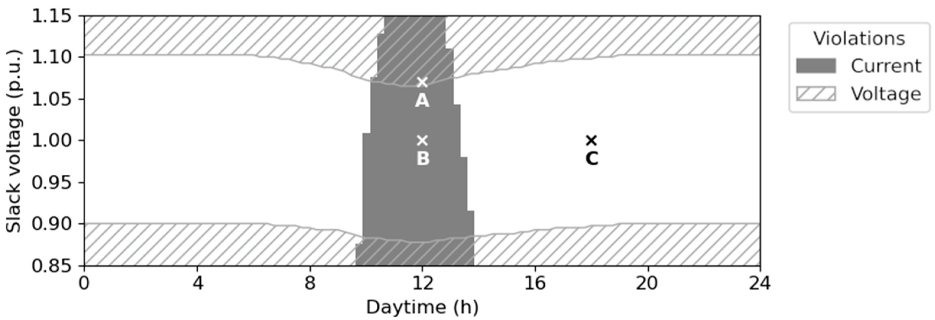
2.1.1. Boundary Voltage Limits

The ESLM complements the model structure given in Equation (2) by new parameters, i.e., the upper and lower BVLs, which allow for validating the compliance with the operational voltage and current limits within the represented system part. It relies on a refined BVL definition introduced by this paper as follows:
Definition 1.
Boundary voltage limits specify the upper and lower voltage limits that must be respected at the connection point of the extended static load model to ensure compliance with the voltage and current limits inside the system part that is represented by this load model.
The component-based parameter identification method, detailed in Section 2.1.3, facilitates the computation of BVLs. These limits, which represent the actual voltage constraints at a given network node, are derived from a series of load flow simulations of the subordinate system part. Unlike conventional approaches that assume conservative and time-invariant voltage limits at the MV level based on worst-case scenarios, the proposed methodology explicitly accounts for time-dependent variations in voltage drops and rises within the subordinate LV networks based on the actual load and generation conditions. Consequently, the proposed approach allows for a more accurate validation of limit compliance across the entire distribution network, capturing the dynamic nature of voltage limits at different network nodes over time.

2.1.2. Extended Static Load Model

The proposed ESLM, which is given in Equation (3), describes the load’s active and reactive power contributions as functions of the local voltage and additionally, the local BVLs to be respected at its connection node.
P = H P V
Q = H Q V
V   V max
V   V min
where V min and V max are the minimal and maximal permissible voltages at the load model’s connection node, respectively. If relevant to the planned analyses, additional information may be added to the model, e.g., the active power losses within the represented system part according to Equation (4).
P = H P V
where P is the active power loss and H P is a function. In general, the functions H P , H Q , and H P may be represented by equations (e.g., linear, exponential, polynomial, and comprehensive) or look-up tables [see Table 1], whereby the latter option is applied and analyzed in this paper. The additional parameters V min and V max allow for validating the compliance with the voltage and current limits inside the system part represented by the corresponding ESLM after running a power flow: Limits are respected only if the local voltage at the ESLM’s connection node lies within the permissible voltage range. Otherwise, either the voltage, current, or both limits are violated. However, the ESLM still returns the P and Q values even if the voltages are outside the permissible range.

2.1.3. Component-Based Identification of Model Parameters

The obligatory ( H P , H Q , V max , and V min ) and optional ( H P ) model parameters can be calculated for any power system portion if the corresponding network model and the ESLM parameters of the subordinate elements are known. Figure 1 illustrates the concept by aggregating a fictional power system portion at the “node of aggregation”.
The following component-based identification procedure allows for the identification of the resulting ESLM’s parameters, which are represented by a look-up table similar to Table 1:
4.
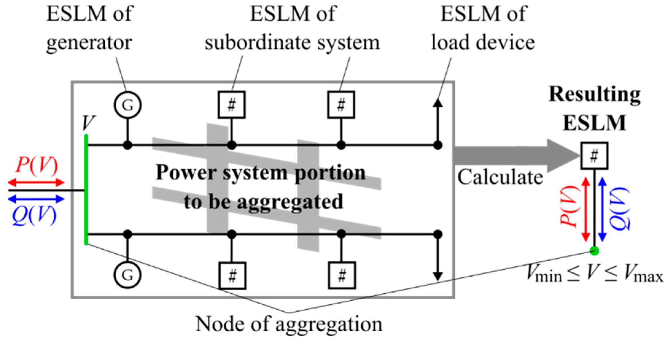
Connect the slack node element to the node of aggregation.
5.
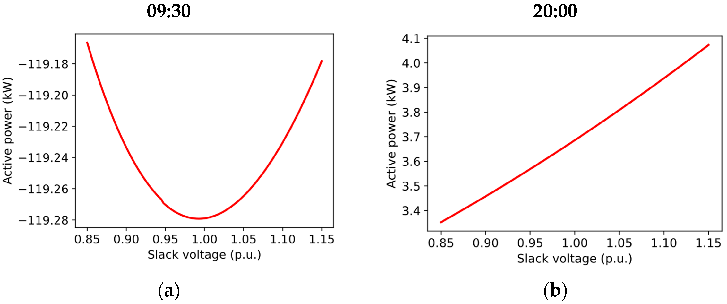
Define the slack voltage range of interest, e.g., from 0.9 to 1.1 p.u., and the corresponding voltage resolution, e.g., 0.0025 p.u. steps.
6.
Repeat load flow simulations for all defined slack voltage values and record the active and reactive power provided by the slack node element as functions of the slack voltage. Furthermore, record all slack voltage values that do not provoke violations of the
  • internal current limits, i.e., current limits of the system portion to be aggregated, or
  • external voltage limits, i.e., BVLs of subordinate ESLMs.
Optionally, record any quantity of interest, such as active power losses according to Equation (5), as functions of the slack voltage.
P V = b P b + i P i V i
where P b and P i are the active power losses of branch b and ESLM i ; V i is the voltage magnitude at the connection node of ESLM i ; and V is the slack voltage. Interpolation is necessary to obtain the values of P i .
This procedure may be repeated for several time intervals to conduct a quasi-static time-series (QSTS) power flow analysis. It yields, for each instance of time, the P V and Q V behavior at the slack node, a set of slack voltages that provokes neither voltage nor current limit violations in the aggregated system portion, and optionally, additional information such as the active power loss as a function of the slack voltage. The upper BVL corresponds to the maximal value in this set, and the lower BVL to the minimal one. If the slack voltage range of interest splits into several permissible areas, BVLs should be specified for each of these areas. Curve-fitting techniques may be used to translate functions H P , H Q , and H P into an equation-based form if desired.
Parallel computation can be used to efficiently aggregate any portion of the power system since all points in the (V, t) plane are independent of each other.

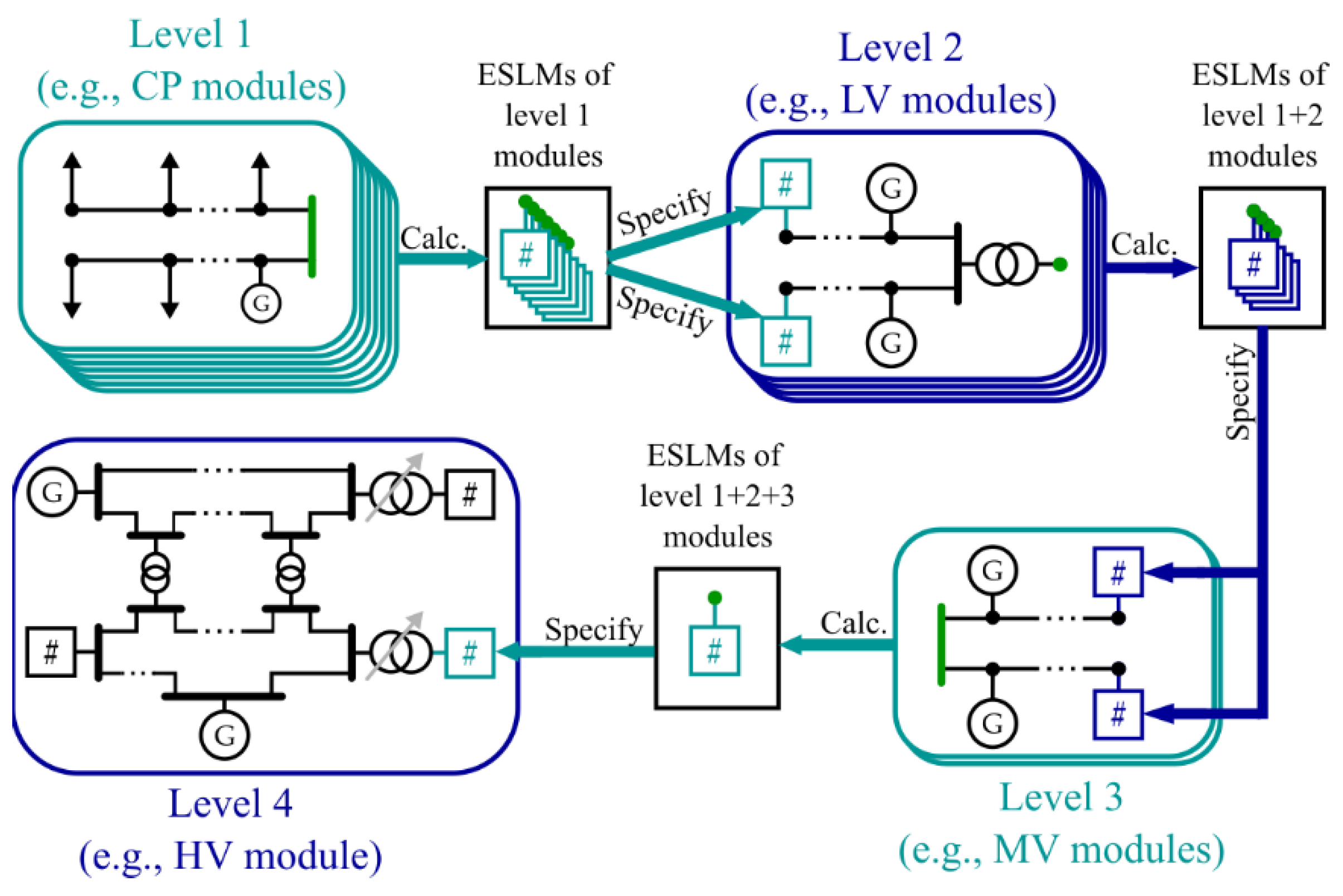
2.2. Modular Power Flow Analysis

The proposed ESLM along with its parameter identification method supports the separate analysis of distinct power system portions, thus offering a modular and systematic approach to power flow analysis.

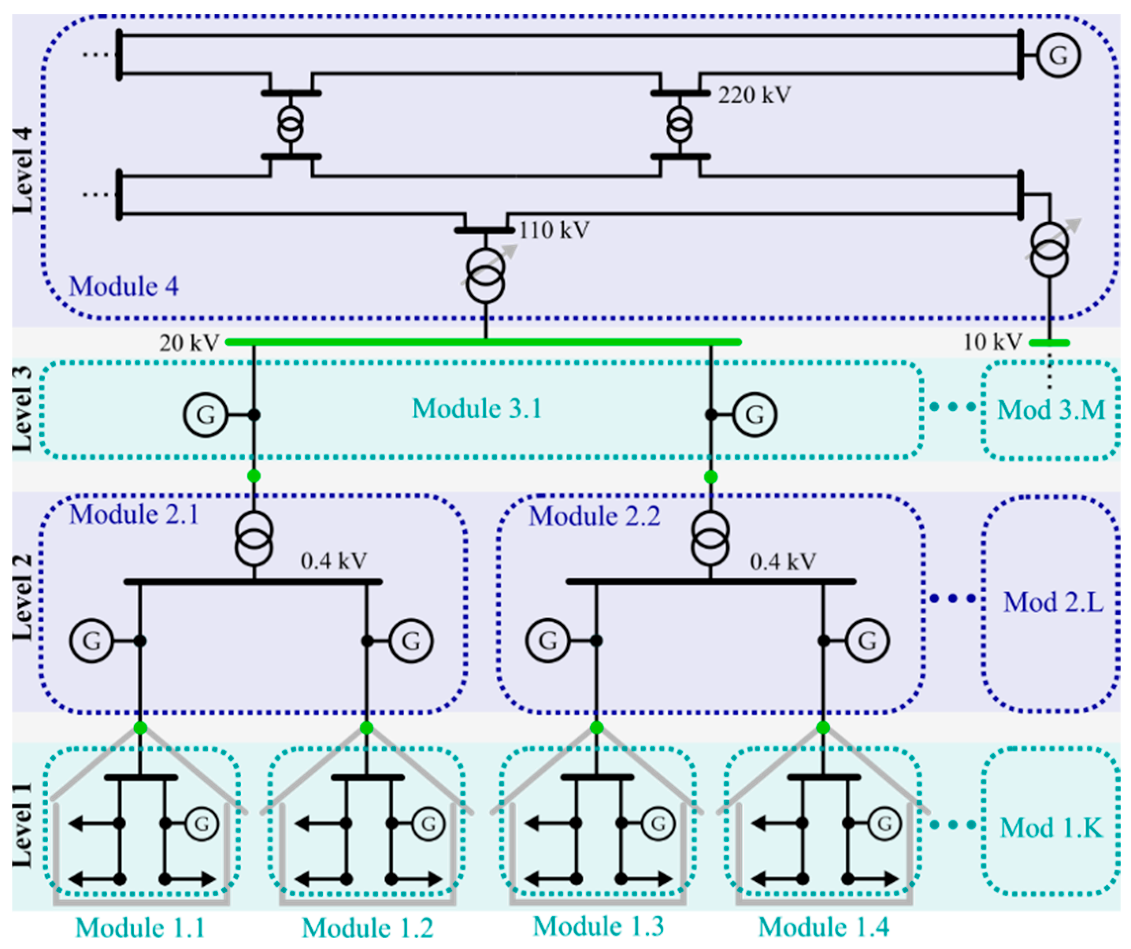
2.2.1. Modularization of the Power System

The first step towards such a modular analysis is splitting the targeted power system into hierarchical levels and further subdividing each level into discrete modules, which are interconnected through so-called “boundary nodes” [see Figure 2]. The hierarchical levels are arranged vertically and characterized by their unique physical dependencies: The state of each module depends on the supplying voltage from the higher-level module and the power contributions from the lower-level ones, in fact without any direct influence from modules at the same level.

2.2.2. Simulation Procedure

The modular approach supports the parallel aggregation of all modules at the same level, while modules that are spread across different levels necessitate sequential aggregation in a bottom-up fashion.
First, the modules situated in the bottom-most level of interest, e.g., the CP modules, are analyzed and aggregated, and the resulting ESLMs are used for the analysis and aggregation of the next-level modules, e.g., the LV modules. This procedure may be repeated several times until each relevant MV-LV-CP chain is modeled by a single ESLM that can be used for the analysis of the HV level [see Figure 3]. The aggregation of the CP modules is optional as their voltage limits are predetermined by standards and do not require calculation, and the effects of the CP-internal network on the resulting load characteristics and losses are usually neglected.

2.2.3. Scope of Applicability

The applicability of the modular power flow analysis is limited by the power system structure and the presence of elements with time-dependent states.
  • Power system structure—Each power system can be divided into arbitrary modules interconnected through single or multiple nodes, although its partitioning along multiple nodes involves significant challenges, as subordinate system parts connected via multiple nodes cannot be accurately represented by conventional and extended static load models (e.g., linear, exponential, or polynomial). This limitation arises because the power flow through each interconnection node depends not only on the voltage magnitudes at all interconnection nodes but also on the phase angle differences between them. Equation (6) illustrates these dependencies for a module with two connection nodes to the superordinate grid without considering the frequency.
P i = H P , i V 1 , V 2 , δ 12 ,         i 1 ,   2
Q i = H Q , i V 1 , V 2 , δ 12 ,       i 1 ,   2
δ 12 = δ 1 δ 2
where i indexes the connection node; P i and Q i are the related active and reactive power flows; V i is the voltage magnitude; δ i is the voltage angle; and H P , i and H Q , i are functions.
  • State variables—Some power system elements that are relevant for power flow analysis have state variables, such as the tap positions of OLTCs and the state of charge of storage systems. In QSTS power flow simulations, these state variables are initialized for the first instance of time and permanently updated according to the power flow results. As the power flow results depend on the used slack voltage, the state variables depend on the complete time and slack voltage history, and consequently, they cannot be described as algebraic functions of (V, t). Hence, the modular approach does not apply to system portions that contain elements with state variables. However, the state variables are often neglected in studies that are not explicitly dedicated to their investigation in order to facilitate the analysis and enable parallel computation. For instance, the time-dependent states of OLTCs are frequently neglected, e.g., by modeling the tap changers as continuous elements that keep the voltage at a specific setpoint, or by initializing the tap position with the same value for each instance of time. Storage units are often represented by node elements with predefined load profiles instead of modeling their state of charge.

2.3. Application Example

The modular power flow approach is applied to a large synthetic distribution system to assess its applicability, effectiveness, and accuracy by comparing it with the conventional power flow approach. This section presents an overview of the test system and details the methodology used for the comparison, whereby Section 3 presents the results of this analysis.

2.3.1. Test System Description

SimBench provides a dataset for electric power systems that includes all network data and all load and generation time series relevant to power flow analysis [28]. One specific distribution system (SimBench code: 1-MV-rural-all-2-no_sw; scenario “lPV”; 1 July 2016), including the MV and LV levels and a 24 h time horizon with low consumption and high photovoltaic production, was selected from this dataset for the following application example. All CPs and distributed generators (DGs) are modeled without any voltage dependencies (constant power). A detailed description of the SimBench dataset can be found in [29].
The rural MV network has a nominal voltage of 20 kV and contains eight feeders with a maximum length of approximately 22.30 km. Its supplying transformer (STR) is removed from the model and the slack node element is directly connected to the supplying substation’s MV bus. A few commercial customer plants and DGs as well as 10 semiurban, 36 small rural, 37 mid-size rural, and 7 large rural LV networks are connected to the MV network. All LV systems of the same type are identical.
The LV system types vary in their distribution transformer (DTR) rating, number of feeders and CPs, and maximal feeder length [see Table 2]. The tap changers of all DTRs are fixed in their mid-positions.

2.3.2. Methodology

The SimBench distribution system described in Section 2.3.1 was analyzed using both modular and conventional power flow approaches [see Figure 4]. The conventional approach simulates the LV and MV levels jointly, serving as a reference to analyzing the accuracy of the modular approach. The modular approach decouples the simulations of both levels, starting with the division of the distribution system into LV and MV modules, followed by their subsequent aggregation. The accuracy of the modular approach is assessed based on the maximum errors in active power flows, reactive power flows, loadings, voltage magnitudes, and voltage angles at the MV level [see Equation (7)]. The ESLMs of the LV subsystems are calculated with various voltage resolutions to assess their impact on accuracy and the used load flow program (DIgSILENT PowerFactory 2023 SP3) was configured for exceptionally high precision (The maximal error of nodal and model equations is set to 1 W and 0.0001%, respectively.) to enable a meaningful comparison between both approaches.
E P max t = max b P b conv t P b mod t
E Q max t = max b Q b conv t Q b mod t
E loading max t = max b loading b conv t loading b mod t
E V max t = max n V n conv t V n mod t
E δ max t = max n δ n conv t δ n mod t
where t is an instance of time; P b conv and Q b conv are the active and reactive power flows through MV branch b calculated with the conventional approach; P b mod and Q b mod are the active and reactive power flows through MV branch b calculated with the modular approach; loading b conv is the loading of MV branch b calculated with the conventional approach; loading b mod is the loading of MV branch b calculated with the modular approach; V n conv and δ n conv are the voltage magnitude and angle at MV node n calculated with the conventional approach; V n mod and δ n mod are the voltage magnitude and angle at MV node n calculated with the modular approach; and E P max , E Q max , E loading max , E V max , and E δ max are the maximum absolute discrepancies in active power, reactive power, loading, voltage magnitude, and voltage angle, respectively, between both approaches.
The possible analyses shown in the grey box in Figure 4 are not executed in this paper but illustrate the usefulness of the modular approach: The ESLMs of the LV modules may be used for an in-depth analysis of the MV module. For instance, the MV module may be simulated for different control strategies of directly connected DGs or for different reinforcement stages without having to recalculate the LV systems for each strategy or stage. Similarly, the ESLM of the MV module may be used to conduct n-1 security and static voltage stability analysis (or any other type of analysis) of the HV module without having to recalculate the MV-LV chain for each contingency scenario or point along the PV and VQ curves.
Figure 5 opposes the conventional and modular power flow approaches applied to the SimBench test system. In the conventional approach, the MV and LV levels are jointly simulated (here, with a slack voltage of 1.00 p.u.) [see Figure 5a]. In the modular approach, the system is divided into 90 LV modules of four types (36 small rural, 37 mid-size rural, 7 large rural, and 10 semiurban) and one MV module [see Figure 5b]. Each LV module consists of LV feeders, CPs, and a distribution transformer, while the MV module includes MV feeders, CPs, DGs, and 90 ESLMs of the subordinate LV systems. Each LV module type is aggregated based on the procedure described in Section 2.1.3 to identify its ESLM parameters according to Equation (3). The resulting ESLMs represent the LV systems in the MV module aggregation, which yields the ESLM parameters of the entire distribution system.
Section 3.3 analyzes the impact of distribution system non-linearities on the accuracy of the modular power flow approach and the impact of the voltage resolution used to aggregate subsystems with the component-based parameter identification method described in Section 2.1.3. This analysis uses the Pearson correlation coefficient as an indicator of the linearity of the P V and Q V characteristics of LV subsystems. Equation (8) defines the Pearson correlation coefficient for a bivariate set ( x 1 , y 1 ) , , x n , y n with n samples [30].
r x y = cov x y σ x σ y = 1 n i = 1 n x i x ¯ y i y ¯ 1 n i = 1 n x i x ¯ 2 1 n i = 1 n y i y ¯ 2
where cov x y is the covariance; σ x and x ¯ are the standard deviation and mean of { x 1 , , x n } ; and σ y and y ¯ are the standard deviation and mean of set { y 1 , , y n } .

3. Results

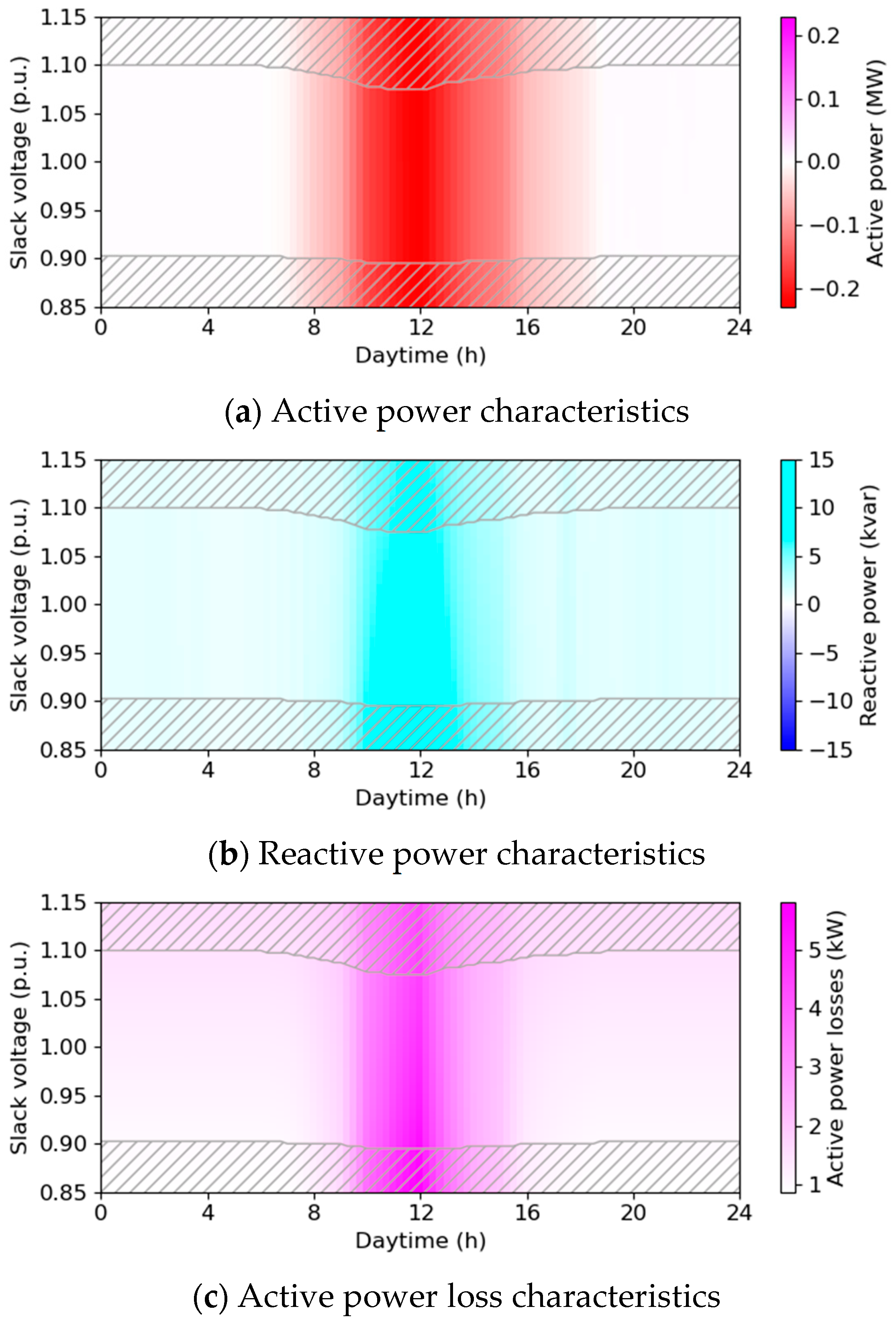
3.1. Aggregation of the LV Level

Using the procedure described in Section 2.1.3 to aggregate the small rural LV module at its boundary node, i.e., the primary bus of its DTR, shows that current limit violations occur around midday; the higher the slack voltage, the shorter the overloading duration [see Figure 6]. The PV injections significantly deform the upper and lower voltage limits around midday: both limits are decreased due to the LV-internal voltage rise.
The meaning of these BVLs becomes clear when analyzing the state of the small rural LV network for three distinct cases [see Figure 7]. Both the voltage and current limits are violated at 12:00 for a slack voltage of 1.07 p.u. (case A) as the DTR is loaded by 132.98% and two DPs violate their upper voltage limit. When the slack voltage is moved to 1.00 p.u. (case B), the DTR loading increases to 141.84% and the DPs do not violate their voltage limits. In case C, where the time and slack voltage are set to 18:00 and 1.00 p.u., respectively, neither current nor voltage limit violations occur.
By changing the DTR rating from 160 kVA to 250 kVA and aggregating the small rural LV network once again, all current limit violations within the regarded (V, t) plane are removed through the transformer replacement [see Figure 8]. The lower and upper voltage limits are only slightly deformed due to the small impedances of the short feeders and the large DTR, reaching 0.895 and 1.075 p.u., respectively, at 12:00. The active and reactive power flows at the DTR’s primary side and the active power losses are dominated by their time dependency: high power flows and losses occur around midday, i.e., when the PV systems inject active power.

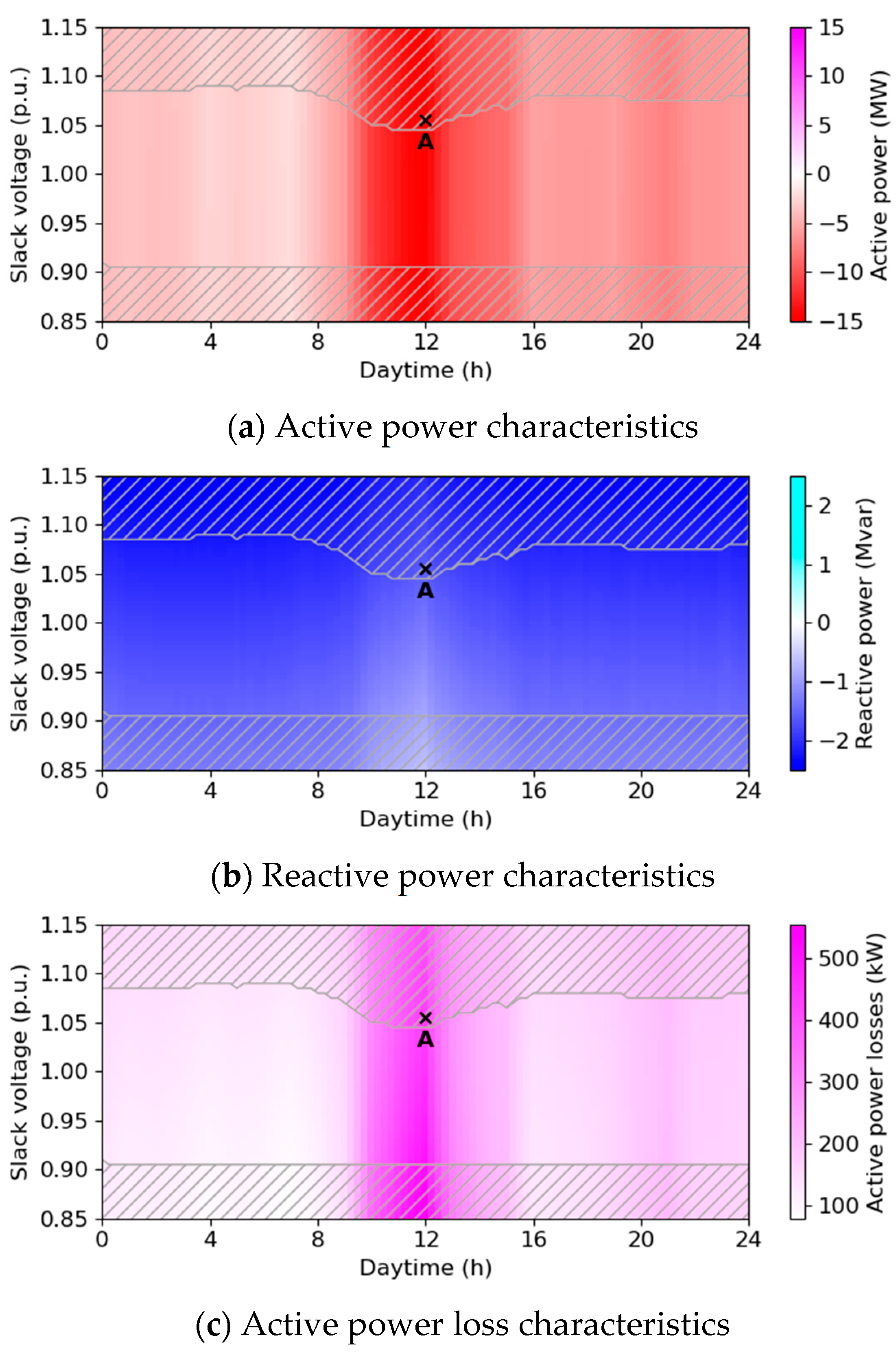
3.2. Aggregation of the MV Level

After aggregating all relevant LV modules, their ESLMs are connected to the rural MV network, which is, as a further consequence, aggregated at its boundary node (bus at the secondary side of STR). Again, the resulting power flows and losses have a significant time dependency, and the upper voltage limit is deformed around midday [see Figure 9]. A capacitive behavior with a noticeable voltage dependency is observed due to the capacitances of the MV cables: the higher the slack voltage, the more the reactive power flows into the HV level.
Analyzing the MV network state for case A, where time and slack voltage are set to 12:00 and 1.055 p.u., respectively, clarifies that each ESLM may have individual BVLs [see Figure 10]. Several small rural and semiurban LV networks violate their upper voltage limits of 1.075 and 1.080 p.u., respectively. As all systems of the same type, e.g., “Small rural LV”, have the same upper voltage limit as they are modelled to be completely identical [see Section 2.3.1], this results in four horizontal lines for the four regarded types. No current limit violations are detected at the MV level, and no customer plant, mid-size, and large rural LV networks violate their upper voltage limits. However, due to the above-mentioned violations, case A exceeds the upper voltage limit seen from the bus at the secondary side of the supplying substation.

3.3. Calculation Accuracy at the MV Level

Figure 11 compares the MV-level results obtained from the modular and conventional power flow approaches for different voltage resolutions of the LV-representing ESLMs. The comparison reveals only marginal discrepancies between the two approaches across the simulated scenarios and for the investigated voltage resolutions of 0.0025, 0.01, and 0.04 p.u. As shown in Figure 11a–c, the discrepancies in active power flow, reactive power flow, loading, voltage magnitude, and voltage angle computations—quantified using Equation (7a–e)—do not exceed 39.11 W, 83.51 var, 8.62 × 10⁻⁴%, 8.62 × 10⁻⁷ p.u., and 4.30 × 10⁻⁵ degrees, respectively, over the considered time horizon. The negligibly small errors across all analyzed metrics confirm the high accuracy of the modular approach in the simulated scenarios.
In Figure 11, a notable impact of the voltage resolution on the discrepancies is observed primarily during noon, but not throughout the remaining time horizon. To understand the underlying cause, we analyze the linearity of the P V and Q V characteristics of the LV subsystems for each instant of time, using the magnitude of the Pearson correlation coefficient as a linearity indicator. A coefficient magnitude of one indicates a perfectly linear relationship, while zero denotes no linearity. Figure 12 shows strong non-linearities in the P V characteristics of small rural and semiurban LV grids during noon. Notably, for the small rural LV system, the magnitude of the Pearson correlation coefficient reaches its minimum value of 0.000061 at 09:30. These non-linearities lead—in the corresponding period—to a significant influence of the voltage resolution of the LV-subsystem representing ESLMs on the discrepancies observed in Figure 11. In contrast, during the remaining time horizon, the impact is low, as the P V and Q V characteristics of the LV subsystems are almost perfectly linear. Figure A2 in Appendix A further illustrates the different levels of non-linearity at different timepoints by comparing the P(V) characteristics of the small rural LV system at 09:30 and 20:00.
This analysis clearly demonstrates that a higher voltage resolution should be applied to highly non-linear systems to obtain accurate results.

4. Discussions

The introduced extended static load model (ESLM) can represent—like the conventional static load model—any power system portion with a single connection node that does not contain any elements with state variables, such as OLTCs and storage. Its component-based parameter identification method adequately considers network losses and spatial voltage variations and enables modular power flow analysis, which supports the systematic, accurate, and computationally practicable analysis of extensive distribution systems. The provided application example showcases the use of the modular power flow approach and indicates that it introduces insignificant inaccuracies.

4.1. Accurate Computation of Power Flows

The conventional approach to the power flow analysis of extensive distribution networks relies on simplified aggregation that neglects network effects like losses and spatial voltage variations of subordinate system parts, leading to inaccuracies, particularly with voltage-dependent elements such as Volt/var-controlled PV inverters. In contrast, the modular approach allows for the separate and sequential simulation of different system parts, maintaining accuracy when the voltage resolution used for subsystem aggregation is appropriately aligned with the system’s linearity. The case study conducted demonstrates negligible discrepancies between the conventional and modular approaches.

4.2. Validation of Compliance with Actual Limits

The modular approach offers the advantage of enabling the systematic validation of voltage and current limit compliance across the entire distribution network. By incorporating boundary voltage limits into the static load model, it allows for the explicit verification of these limits during sequential simulations of different system levels, overcoming the limitations of conventional static load models, which cannot validate compliance in subordinate system parts and usually assumes conservative voltage limits at the MV level instead of calculating the actual ones.

4.3. Systematization of Power Flow Studies

The modular approach allows for reducing computational overhead in studies that involve repeated power flow simulations under variation in a few parameters, such as n-1 security analysis, static voltage stability assessment, and network reinforcement as well as control parametrization studies. By aggregating system parts that remain unchanged during the study only once and representing them by ESLMs, the system part subject to parameter variations can be isolated and studied as needed. This approach allows for the simulation of various parameter settings without the need to recalculate power flows in the aggregated system parts again and again.

4.4. Computational Effort and Performance

The proposed ESLM and modular power flow approach support the separate analysis of distinct system modules and the comprehensive parallelization of the necessary computations. They offer users the freedom to tailor these modules according to specific memory constraints. When aggregating a single module, all points in the relevant (V, t) plane can be computed in parallel. Furthermore, the parallel aggregation of all modules situated at the same level is possible as soon as the ESLM parameters of the subordinate systems are known. This high degree of parallelizability ensures maximal scalability of the modular approach.
The computational performance of the modular power flow approach relative to the conventional method depends on factors such as the voltage resolution, the number of available cores for parallel computation, and the specific use case. In studies involving repeated calculations with minor parameter variations, the pre-aggregation of unchanged system parts can significantly reduce computation time, depending on the frequency of recalculations and the size of the unchanged system parts. For instance, in a network reinforcement study where the MV level is incrementally upgraded based on power flow results (as presented in [31]), pre-aggregating the LV networks using the proposed method may accelerate the computations depending on the prevalent conditions. The extent of the performance gain depends on the number and size of LV networks connected to the MV network, the number of cores available for pre-aggregation, and the number of simulation runs required to determine the final reinforcement needs of the MV network.

4.5. Limitations

The extended static load model—like the conventional one—allows for representing subordinate system parts that are connected through a single boundary node and do not contain elements with state variables, such as storage and on-load tap changers. However, in studies that are not explicitly dedicated to the analysis of these states, these state variables are usually not explicitly modeled to simplify the analysis and enable parallel computations, making the modular approach applicable in these cases.

4.6. Future Work

Future work should focus on conducting a systematic large-scale simulation study to assess the sensitivity of the modular approach’s inaccuracies and computational performance to various conditions. These conditions should encompass systems with different levels of nonlinearity, arising from diverse network configurations (including real datasets), load characteristics, and control setups. Additionally, different use cases should be considered to quantify the performance gains across various types of studies.

5. Conclusions

Simulating power flows in distribution networks across high, medium, and low voltage levels is computationally infeasible due to the large number of nodes and branches. Studies therefore focus on a single or few levels, representing subordinate system parts with conventional static load models. These models do not support the validation of voltage and current limit compliance within the represented system parts, and their parameters are identified through simplified aggregation methods that neglect network effects such as losses and spatial voltage variations, which may lead to significant errors in the presence of voltage-dependent controls. Moreover, in studies requiring repeated simulations with only minor parameter variations—such as n-1 security analysis, static voltage stability assessment, network reinforcement, and control parametrization—the conventional approach lacks a systematic and accurate method to avoid redundant computations within unchanged system parts.
The extended static load model, combined with its component-based parameter identification method, introduces a modular approach to power flow analysis that overcomes these limitations. By incorporating boundary voltage limits, it enables the validation of voltage and current constraints within the represented system part. The parameter identification method ensures accurate aggregation by explicitly considering network losses and spatial voltage variations. Applied iteratively in a bottom-up manner, the modular approach facilitates the analysis of large distribution systems that cannot be simulated as a whole. It provides a systematic means to aggregate system parts that remain unchanged, reducing computational overhead in studies involving repeated simulations under minor parameter adaptations. Additionally, its highly parallelizable structure ensures maximal scalability by facilitating the parallel model parameter computation of a single subsystem, as well as the parallel aggregation of multiple subsystems at the same level.
Future work should focus on a large-scale simulation study to evaluate the inaccuracies and computational performance of the modular versus the conventional approach under various conditions.

Author Contributions

Conceptualization, D.-L.S.; methodology, D.-L.S.; software, D.-L.S.; validation, C.K.; formal analysis, D.-L.S.; investigation, D.-L.S.; writing—original draft preparation, D.-L.S.; writing—review and editing, C.K.; visualization, D.-L.S. All authors have read and agreed to the published version of the manuscript.

Funding

This research received no external funding.

Data Availability Statement

The original data presented in the study are openly available in Mendeley Data at https://data.mendeley.com/datasets/pmhjvpn9d3/1 (accessed on 18 March 2025).

Acknowledgments

The authors acknowledge Barbara Herndler for her assistance in reviewing and improving the English language of this manuscript.

Conflicts of Interest

Author Daniel-Leon Schultis was employed by the company Magnus Energy B.V. The remaining authors declare that the research was conducted in the absence of any commercial or financial relationships that could be construed as a potential conflict of interest.

Abbreviations

The following abbreviations are used in this manuscript:
BVLBoundary voltage limit
CPCustomer plant
DGDistributed generator
DPDelivery point
DTRDistribution transformer
ESLMExtended static load model
HVHigh voltage
LVLow voltage
MVMedium voltage
OLTCOn-load tap changer
PVPhotovoltaic
QSTSQuasi-static time-series
STRSupplying transformer

Appendix A

Equations (A1)–(A5) describe the basic principles of the simplified procedure commonly used for the component-based load aggregation. In accordance with Equation (2), the individual loads distributed along a radial feeder, as well as the aggregate load observed at the feeder’s origin, can be mathematically represented by Equations (A1) and (A2) as voltage-dependent power contributions [see Figure A1].
P 0 = P n , 0 · h P , 0 V 0
Q 0 = Q n , 0 · h Q , 0 V 0
P i = P n , i · h P , i V i         i 1 ,   N
Q i = Q n , 0 · h Q , i V i         i 1 ,   N
where N is the number of loads.
Figure A1. Radial feeder with N loads.
Energies 18 01559 g0a1
Equation (A3) ignores the feeder losses and determines the aggregate load model by superimposing the individual models.
P 0 = i = 1 N P i
Q 0 = i = 1 N Q i
Neglecting spatial voltage variations ( V 0 = V i = V ), which are significant in distribution networks, allows for the calculation of the aggregate load at nominal voltage and the associated voltage dependency terms according to Equations (A4) and (A5).
P n , 0 = i = 1 N P n , i
Q n , 0 = i = 1 N Q n , i
h P , 0 V = i = 1 N P n , i · h P , i V / i = 1 N P n , i
h Q , 0 V = i = 1 N Q n , i · h Q , i V / i = 1 N Q n , i
Figure A2 shows that the P(V) characteristic of the small rural LV system is strongly non-linear at 09:30 and almost linear at 20:00.
Figure A2. P V characteristic at the primary side of the small rural LV system’s 250 kVA DTR at 09:30 (a) and 20:00 (b).
Energies 18 01559 g0a2

References

  1. Martinez, J.A.; Mahseredjian, J. Load Flow Calculations in Distribution Systems with Distributed Resources. A Review. In Proceedings of the 2011 IEEE Power and Energy Society General Meeting, Detroit, MI, USA, 24–28 July 2011; pp. 1–8. [Google Scholar]
  2. Price, W.W.; Chiang, H.-D.; Clark, H.K.; Concordia, C.; Lee, D.C.; Hsu, J.C.; Ihara, S.; King, C.A.; Lin, C.J.; Mansour, Y.; et al. Load Representation for Dynamic Performance Analysis (of Power Systems). IEEE Trans. Power Syst. 1993, 8, 472–482. [Google Scholar] [CrossRef]
  3. Arif, A.; Wang, Z.; Wang, J.; Mather, B.; Bashualdo, H.; Zhao, D. Load Modeling—A Review. IEEE Trans. Smart Grid 2018, 9, 5986–5999. [Google Scholar] [CrossRef]
  4. Modelling and Aggregation of Loads in Flexible Power Networks. Available online: https://e-cigre.org/publication/566-modelling-and-aggregation-of-loads-in-flexible-power-networks (accessed on 5 May 2022).
  5. Standard Load Models for Power Flow and Dynamic Performance Simulation. IEEE Trans. Power Syst. 1995, 10, 1302–1313. [CrossRef]
  6. Schultis, D.-L.; Petrusic, S.; Ilo, A. Modelling of Low-Voltage Grids with High PV Share and Q(U)-Control. CIRED Open Access Proc. J. 2021, 2020, 501–504. [Google Scholar] [CrossRef]
  7. IEEE Std 2781-2022; IEEE Guide for Load Modeling and Simulations for Power Systems. IEEE: Piscataway, NJ, USA, 2022; pp. 1–88. [CrossRef]
  8. Ren, H.; Schulz, N.N.; Krishnan, V.; Zhang, Y. Online Static Load Model Estimation in Distribution Systems. In Proceedings of the 2019 IEEE 28th International Symposium on Industrial Electronics (ISIE), Vancouver, BC, Canada, 12–14 June 2019; pp. 153–158. [Google Scholar]
  9. Wang, C.; Wang, Z.; Wang, J.; Zhao, D. Robust Time-Varying Parameter Identification for Composite Load Modeling. IEEE Trans. Smart Grid 2019, 10, 967–979. [Google Scholar] [CrossRef]
  10. Ballanti, A.; Ochoa, L.F. Initial Assessment of Voltage-Led Demand Response from UK Residential Loads. In Proceedings of the 2015 IEEE Power & Energy Society Innovative Smart Grid Technologies Conference (ISGT), Washington, DC, USA, 18–20 February 2015; pp. 1–5. [Google Scholar]
  11. Lamberti, F.; Dong, C.; Calderaro, V.; Ochoa, L.F. Estimating the Load Response to Voltage Changes at UK Primary Substations. In Proceedings of the IEEE PES ISGT Europe 2013, Lyngby, Denmark, 6–9 October 2013; pp. 1–5. [Google Scholar]
  12. Ballanti, A.; Ochoa, L.F. Voltage-Led Load Management in Whole Distribution Networks. IEEE Trans. Power Syst. 2018, 33, 1544–1554. [Google Scholar] [CrossRef]
  13. Schultis, D.-L.; Ilo, A. Adaption of the Current Load Model to Consider Residential Customers Having Turned to LED Lighting. In Proceedings of the 2019 IEEE PES Asia-Pacific Power and Energy Engineering Conference (APPEEC), Macao, China, 1–4 December 2019; pp. 1–5. [Google Scholar]
  14. Collin, A.J.; Tsagarakis, G.; Kiprakis, A.E.; McLaughlin, S. Development of Low-Voltage Load Models for the Residential Load Sector. IEEE Trans. Power Syst. 2014, 29, 2180–2188. [Google Scholar] [CrossRef]
  15. Collin, A.J.; Acosta, J.L.; Hayes, B.P.; Djokic, S.Z. Component-Based Aggregate Load Models for Combined Power Flow and Harmonic Analysis. In Proceedings of the 7th Mediterranean Conference and Exhibition on Power Generation, Transmission, Distribution and Energy Conversion (MedPower 2010), Agia Napa, Cyprus, 7–10 November 2010; pp. 1–10. [Google Scholar]
  16. Tang, Y.; Zhang, H.-B.; Zhang, D.-X.; Hou, J.-X. A Synthesis Load Model with Distribution Network for Power Transmission System Simulation and Its Validation. In Proceedings of the 2009 IEEE Power & Energy Society General Meeting, Calgary, AB, Canada, 26–30 July 2009; pp. 1–7. [Google Scholar]
  17. Chen, Q.; Ju, P.; Shi, K.Q.; Tang, Y.; Shao, Z.Y.; Yang, W.Y. Parameter Estimation and Comparison of the Load Models with Considering Distribution Network Directly or Indirectly. Int. J. Electr. Power Energy Syst. 2010, 32, 965–968. [Google Scholar] [CrossRef]
  18. Wang, Q.; Zhao, B.; Ren, B.; Li, Q.; Hao, J.; Lan, T.; Luo, P. Synthetic Load Modelling Considering the Influence of Distributed Generation. Energy Rep. 2023, 9, 662–669. [Google Scholar] [CrossRef]
  19. Wu, P.; Zhang, X.; Lu, C.; Wang, Y.; Ye, H.; Ling, X. A Composite Load Model Aggregation Method and Its Equivalent Error Analysis. Int. J. Electr. Power Energy Syst. 2023, 150, 109098. [Google Scholar] [CrossRef]
  20. Joshi, K.; Pindoriya, N. Advances in Distribution System Analysis with Distributed Resources: Survey with a Case Study. Sustain. Energy Grids Netw. 2018, 15, 86–100. [Google Scholar] [CrossRef]
  21. Power Distribution in Europe—Facts & Figures. Available online: https://www3.eurelectric.org/powerdistributionineurope/ (accessed on 4 October 2023).
  22. Turiman, M.S.; Sarmin, M.K.N.M.; Saadun, N.; Chong, L.C.; Ali, H.; Mohammad, Q. Analysis of High Penetration Level of Distributed Generation at Medium Voltage Levels of Distribution Networks. In Proceedings of the 2022 IEEE International Conference on Power Systems Technology (POWERCON), Kuala Lumpur, Malaysia, 12–14 September 2022; pp. 1–6. [Google Scholar]
  23. Arshad, A.; Lehtonen, M. Multi-Agent System Based Distributed Voltage Control in Medium Voltage Distribution Systems. In Proceedings of the 2016 17th International Scientific Conference on Electric Power Engineering (EPE), Prague, Czech Republic, 16–18 May 2016; pp. 1–6. [Google Scholar]
  24. Jayasekara, N.; Masoum, M.A.S.; Wolfs, P.J. Optimal Operation of Distributed Energy Storage Systems to Improve Distribution Network Load and Generation Hosting Capability. IEEE Trans. Sustain. Energy 2016, 7, 250–261. [Google Scholar] [CrossRef]
  25. OVE EN 50160; Voltage Characteristics of Electricity Supplied by Public Electricity Networks. Austrian Standards: Vienna, Austria, 2020. Available online: https://www.austrian-standards.at/de/shop/ove-en-50160-2020-12-01~p2557383 (accessed on 25 June 2024).
  26. Bolgaryn, R.; Scheidler, A.; Braun, M. Combined Planning of Medium and Low Voltage Grids. In Proceedings of the 2019 IEEE Milan PowerTech, Milan, Italy, 23–27 June 2019; pp. 1–6. [Google Scholar]
  27. Schultis, D.-L.; Ilo, A. Increasing the Utilization of Existing Infrastructures by Using the Newly Introduced Boundary Voltage Limits. Energies 2021, 14, 5106. [Google Scholar] [CrossRef]
  28. Meinecke, S.; Sarajlić, D.; Drauz, S.R.; Klettke, A.; Lauven, L.-P.; Rehtanz, C.; Moser, A.; Braun, M. SimBench—A Benchmark Dataset of Electric Power Systems to Compare Innovative Solutions Based on Power Flow Analysis. Energies 2020, 13, 3290. [Google Scholar] [CrossRef]
  29. Meinecke, S.; Bornhorst, N.; Lauven, L.-P.; Menke, J.-H.; Braun, M.; Drauz, S.; Spalthoff, C.; Cronbach, D.; Kneiske, T.; Klettke, A.; et al. SimBench—Dokumentation. Available online: https://simbench.de/wp-content/uploads/2021/09/simbench_documentation_de_1.1.0.pdf (accessed on 11 February 2025).
  30. Obilor, E.I.; Amadi, E. Test for Significance of Pearson’s Correlation Coefficient (r). Int. J. Innov. Math. Stat. Energy Policies 2018, 6, 11–23. [Google Scholar]
  31. Brunner, H.; Korner, C.; Wieland, T.; Brandl, S.; Ortner, M. Methods and Future Scenarios for Strategic Grid Development of Full Low and Medium Voltage DSO Supply Areas. IET Conf. Proc. 2023, 2023, 2872–2876. [Google Scholar] [CrossRef]
Figure 1. Illustration of the component-based ESLM parameter identification method. The node of aggregation is marked in green.
Energies 18 01559 g001
Figure 2. Exemplary modularization of a fictional power system. The boundary nodes, which interconnect the modules, are marked in green. Levels one, two, and three contain K, L, and M modules, respectively, and level four constitutes a single module.
Energies 18 01559 g002
Figure 3. Illustration of the modular simulation procedure. Nodes of aggregation are marked in green.
Energies 18 01559 g003
Figure 4. Methodology used to showcase the modular power flow approach and analyze its accuracy.
Energies 18 01559 g004
Figure 5. Illustration of different power flow approaches applied to the selected SimBench distribution system: (a) conventional and (b) modular. In sub-figure (b), the boundary nodes, which correspond to the nodes of aggregation, are marked in green, and while system parts are symbolized as # .
Energies 18 01559 g005
Figure 6. BVLs of the ESLM representing the small rural LV network with a 160 kVA DTR. Gray shading and hatched areas indicate areas where current and voltage limit violations occur, respectively. Cases A, B, and C are subsequently used for detailed network state analysis.
Energies 18 01559 g006
Figure 7. Voltage profiles and branch loadings of the small rural LV network with a 160 kVA DTR for different cases: (a) case A; (b) case B; (c) case C. The delivery points of customers are marked by black dots and the upper voltage limit is indicated with a horizontal black line in (a). The vertical line at zero distance shows the voltage drop or rise over the DTR.
Energies 18 01559 g007
Figure 8. Mandatory ((a) active power and (b) reactive power load characteristics and BVLs) and optional ((c) active power losses) ESLM parameters seen from the distribution substation (primary bus) of the small rural LV network with a 250 kVA DTR. Negative active and reactive power values indicate an injection into the MV network, and vice versa. Areas where voltage limit violations occur at the LV level are marked by gray hatched areas. No current limit violations are detected.
Energies 18 01559 g008
Figure 9. Mandatory ((a) active power and (b) reactive power load characteristics and BVLs) and optional ((c) active power losses) ESLM parameters seen from the supplying substation (secondary bus) of the rural MV network. Negative active and reactive power values indicate an injection into the HV network, and vice versa. Areas where voltage limit violations occur at the MV level are marked by gray hatched areas. No current limit violations are detected. Case A is subsequently used for detailed network state analysis.
Energies 18 01559 g009
Figure 10. Voltage profiles and branch loadings of the rural MV network for case A. The delivery points of customers are marked by black dots and the connection points of small rural, mid-size rural, large rural, and semiurban LV networks are marked by purple pluses (+), blue asterisks (*), magenta pentagons (⬟), and brown diamonds (♦), respectively. The upper voltage limits valid for 12:00 are shown by horizontal lines in the respective colors.
Energies 18 01559 g010
Figure 11. Maximum discrepancies in active power flow (a), reactive power flow (b), loading (c), voltage magnitude (d), and voltage angle computations (e) at the MV level between the conventional and modular power flow approach. In the modular approach, the LV subsystems are represented by ESLMs, whereas in the conventional approach, they are modeled in full detail. The solid, hatched, and dotted lines indicate the errors for different voltage resolutions of the LV-representing ESLMs, i.e., 0.0025, 0.0100, and 0.0400 p.u.
Energies 18 01559 g011
Figure 12. Magnitude of the Pearson correlation coefficient between voltage and active power (red) as well as voltage and reactive power (blue) at the primary side of the DTR over time for the small rural with a 250 kVA DTR (a), mid-size rural (b), large rural (c), and semiurban LV networks (d).
Energies 18 01559 g012
Table 1. Look-up table including the active and reactive power contributions, active power losses, and BVLs of an ESLM representing an exemplary LV system with significant photovoltaic generation at midday as functions of voltage. Negative power values correspond to an injection into the superordinate MV network and vice versa.
V m i n (p.u.) V m a x (p.u.) V (p.u.) P (kW) Q (kvar) P (kW)
0.8581.0751.100−228.778.244.46
1.095−228.758.314.48
0.905−227.8611.535.37
0.900−227.8211.645.41
Table 2. Overview of the relevant LV systems.
TypeDTR Rating (kVA)No. FeedersMax. Feeder Length (m)Number of CPs
Small rural160 or 2504245.3413
Mid-size rural2504564.6999
Large rural4009479.34118
Semiurban4003228.9841
Disclaimer/Publisher’s Note: The statements, opinions and data contained in all publications are solely those of the individual author(s) and contributor(s) and not of MDPI and/or the editor(s). MDPI and/or the editor(s) disclaim responsibility for any injury to people or property resulting from any ideas, methods, instructions or products referred to in the content.

