Quantifying the Economic Advantages of Energy Management Systems for Domestic Prosumers with Electric Vehicles

Abstract

The increasing adoption of intermittent renewable energy sources and electric vehicles in households necessitates effective energy management systems (EMS) in the residential sector. This study quantifies the economic benefits of using a state-of-the-art EMS for optimally controlling a grid-connected smart home, which includes PV panels, a battery, and an EV charging station with either monodirectional or bidirectional charging modes. The EMS uses a two-layer approach: the first layer handles strategic decisions with day-ahead forecasts and solving a mixed-integer linear program (MILP) model; the second layer manages the real-time control decisions based on a heuristic strategy. Tested on 396 real-world case studies (based on measured data) with varying user types and energy systems (different PV plant sizes, with or without BESS, and different EV charging modes), different EV models, and weekly commutes, the results demonstrate the EMS’s cost-effectiveness compared to current non-predictive heuristic strategies. Annual cost savings exceed 20% in all cases and reach up to 900 €/year for configurations with large (6 kW) PV plants. Additionally, while installing a battery is not economically advantageous, bidirectional EV chargers yield 10–15% additional savings compared to monodirectional chargers, increasing with more weekly remote working days.

1. Introduction

The objectives to reach climate neutrality by 2050 are pushing the spread of renewable energy sources (RES) generation and the penetration of electric vehicles (EV), strongly affecting the residential environment. In the EU, the Commission has introduced the EU Solar Energy Strategy as part of the REPowerEU plan, aiming to accelerate the deployment of solar technologies. The objective is to install over 320 GW of solar photovoltaic (PV) capacity by 2025 and nearly 600 GW by 2030. To facilitate this transition, the European Solar Rooftop Initiative has been launched to tap into the vast, underutilized potential of rooftops for clean energy production. This initiative includes a phased obligation to install solar panels on various building types, starting with new public and commercial structures and gradually extending to residential buildings [1]. In 2022, rooftop solar photovoltaic (PV) panels contributed an additional 25 GW of capacity, marking an increase of 8 GW compared to 2021. This growth was particularly notable in the residential and small commercial sectors, where investment decisions are made swiftly and system installations are relatively quick to complete [2]. Meanwhile, EV adoption is also accelerating; in June 2023, new battery-electric car registrations in the EU increased by 66.2%, reaching 158,252 units. This boosted their market share to 15.1% (up from 10.7% in June 2022), making EVs the third most popular choice among new car buyers, surpassing diesel for the first time [3].

This evolving landscape of energy systems mandates a critical examination of energy management and control within the residential sector to properly integrate the RES generation with the EV requirements. Presently, the deployment of smart metering systems stands out as a significant opportunity, offering nearly real-time feedback on energy consumption and production. EU is actively promoting the widespread adoption of these systems [4], alongside the integration of energy systems [5], to achieve cost-effective decarbonization of EU economies.

Italy’s Integrated National Energy and Climate Plan [6,7] places citizens and businesses at the center of the green transition, encouraging them to take an active role in the energy transformation. A major challenge is the inefficiency of Italy’s residential building stock, with 55% of homes classified in the lowest energy efficiency categories. To address this, the PNIEC aims to increase renovation rates, promote electrification, and support automation, control, and insulation improvements. One particularly promising avenue for integration is the electrification of transport, which can foster a more flexible, decentralized, and digitalized energy system. However, conventional heuristic management and control strategies currently used in residential energy systems are inadequate for achieving optimal integration between EVs and rooftop PV installations [8].

To overcome these limitations, significant efforts are being directed toward the development of advanced energy management systems (EMSs) based on predictive approaches [9]. This study methodically evaluates the advantages of predictive EMSs over heuristic strategies in residential settings through extensive real-world case studies conducted in collaboration with industrial partners. The following section provides an overview of the EMSs specifically developed for the optimal management of domestic plants.

1.1. Relevant Literature

Numerous studies have explored residential energy management, employing various methodologies to address the challenges in this field [8]. Among these, it is worth mentioning stochastic dynamic programming (SDP), reinforcement learning (RL), and mixed-integer linear programming (MILP). These tools are versatile, applicable not only to the management of individual households but also to broader scales such as buildings, energy communities, or microgrids (MG).

Wu et al. [10,11] utilized SDP to optimize energy management in a smart home with plug-in electric vehicles (PEVs). Particularly suitable for handling uncertainty, SDP in these instances modeled trip time and trip length through probability distributions, resulting in cost savings across various operational modes. RL represents a powerful tool for managing systems with increasing complexity, such as energy communities with a growing number of users, EVs or storage. Shin et al. [12] applied a multi-agent deep RL approach to a system where a single private enterprise managed multiple EV charging stations equipped with renewable energy resources, each independently connected to battery energy storage systems (BESSs). This method effectively reduced the operating costs of the EV charging stations.

Another well-established framework in the smart home EMS is the MILP, which is also the method adopted in this work. Wi et al. [13] developed an EMS based on a MILP optimization module with an intelligent EV charging strategy for smart homes and buildings equipped with PV systems. The implemented EMS effectively aligned EV charging schedules with user preferences. Erdinc [14] employed MILP to assess demand response (DR) strategies in grid-connected smart households, equipped with bi-directional power flow capability EVs and energy storage systems, significantly impacting household power consumption patterns. Paterakis et al. [15] formulated an EMS to optimize day-ahead appliance scheduling while considering hourly electricity pricing and peak power constraints. The model efficiently handled both thermostatically controlled (e.g., air conditioners and water heaters) and non-thermostatically controlled (e.g., washing machines and dishwashers) appliances, along with EVs, proving computationally efficient even in realistic case studies. Tostado-Véliz et al. [16] investigated management strategies for isolated homes adopting a MILP formulation to leverage deferrable loads and vehicle-to-home (V2H) strategies. By jointly adopting these strategies, cost savings of up to 41.5% were achieved compared to a benchmark off-grid residential case. MILP models can be seamlessly integrated into a real-time rolling horizon optimization framework, as shown by Paterakis et al. in [17]. This work proposed a home EMS to minimize energy procurement costs for households enrolled in dynamic pricing tariff schemes. The rolling horizon approach effectively handled uncertainties in PV generation, user consumption, and EV behavior by continuously updating system parameters based on real-time data. In addition, MILP frameworks can be applied to optimally size smart households in terms of RES generation and storage capabilities, as demonstrated by Erdinc et al. in [18]. Pilotti et al. [19] used MILP to optimize the operation of a microgrid featuring an e-fleet parking lot, PV panels, stationary batteries, and industrial loads, highlighting the benefits of participating in energy-intensive reserve programs to align EV charging with service provisioning. Tostado-Véliz et al. [20] effectively addressed uncertainty by developing a stochastic many-objective solution based on MILP, which was tested on a home layout. Tostado-Véliz et al. [21] focused on nearly zero energy buildings, which aim to achieve a yearly near-zero net energy consumption. They exploited a combination of stochastic programming and information-gap decision theory (IGDT) with a modular MILP formulation to minimize various objective functions while preserving robustness and efficiency. Zhang et al. [22] proposed a MILP model to manage smart homes using an MG system to minimize daily energy cost and CO₂ emissions. Residential communities were addressed by Erdinç [23] through a rolling horizon approach that was able to guarantee a fair allocation of shared resources and sustain cost effectiveness. Thomas et al. [24] compared deterministic and stochastic EMS approaches for buildings with EV fleets capable of bidirectional energy trading, confirming that stochastic optimization consistently reduced total daily system costs compared to deterministic alternatives.

EMS architectures typically adopt a hierarchical structure, with layers addressing different time scales and technical aspects of energy management [25]. Upper layers oversee the medium-term operation solving the unit commitment problem that is based on profiles generated by the forecast generation module. Lower layers implement strategic decisions from upper layers, handling real-time system dispatch by acting on its components. Moretti et al. [26] developed a two-layer predictive EMS for an off-grid hybrid MG, integrating controllable and non-controllable generation alongside storage. Tested on a rural MG in Somalia, this strategy achieved significant renewable energy penetration and reduced fuel consumption by 24.1% compared to the best heuristic alternative. Esmaeel Nezhad et al. [27] employ MILP within a shrinking horizon (SH) model predictive control (MPC) framework for a home EMS, targeting the reduction of electricity costs. The case studies analyzed demonstrate that the SH MPC effectively lowers costs and generates profits for prosumers equipped with PV and BESS by optimizing the integration of load-shifting programs, local power generation, and storage systems. This approach proves beneficial under both time-of-use tariffs and real-time pricing schemes. Jiang et al. [28] designed an EMS to enhance the MG reliability. Leveraging coordination between the schedule layer and the dispatch layer, this EMS dynamically allocated and updated an adequate active power reserve for real-time MG dispatch, addressing the indeterminacy of uncontrollable units in both grid-connected and stand-alone modes. Additionally, Fusco et al. [29] utilized a hierarchical EMS to manage a single-bus system comprising PV and BESS assets, optimizing participation in the Italian day-ahead and intra-day electricity markets. The system successfully executed and maintained a sequential bidding strategy through the integration of load and PV forecasts with energy management.

1.2. Motivation and Contribution

The objective of this work is to quantify the economic gain (cost savings) achievable by adopting a state-of-the-art EMS for the optimal operation of a domestic plant consisting of rooftop PV, EV charger (monodirectional or bidirectional), and (optionally) battery energy storage (BESS). The scheme is shown in Figure 1.

Unlike previous studies that focus on the development of novel energy management algorithms, this work is centered on evaluating the financial advantages of EMS implementation. In order to have sufficient statistical relevance, the analysis considers a large number of cases (about 400), all featuring real-world data (measured profiles), and the operation of the domestic plant for the whole year. The case studies cover different user profiles, energy systems (different sizes of the PV plant, with or without BESS, with monodirectional or bidirectional EV charging station), EV models, and weekly commutes, resulting in a total of 396 instances.

The implemented EMS is based on the same structure and state-of-the-art methods adopted in today’s EMS for industrial plans and microgrids. It is structured on two main modules: the forecast module and the optimization module. The forecast module uses artificial intelligence algorithms to predict the production of PV panels and the electricity consumption of the house for the next 24 h. The optimization module is structured in two layers: the first layer is the strategic planning problem (energy flows exchanged between PV, EV, and BESS in the next 24 h), which is modeled and solved as a MILP; the second layer uses a rule-based heuristic strategy to adjust the power exchanged between the different units to meet the current power demands and PV production. The implemented EMS represents the best trade-off between complexity (input data, computational time, and resources required to solve the optimization problem) and optimality. More advanced EMS based on stochastic (e.g., [30,31]) or robust optimization approaches (e.g., [32,33]) require additional input data (e.g., uncertainty set definition or scenarios definition) and may yield computationally intensive problems (requiring expensive MILP solvers and powerful hardware for the calculator), making them not suitable for practical implementation in a domestic plant. To assess the reliability of the proposed framework, the impact of forecast accuracy is thoroughly investigated, identifying the most significant sources of uncertainty affecting economic performance.

The remainder of the paper is structured as follows. Section 2 presents the home EMS. This section covers the hierarchical structure approach and the mathematical formulation describing the first and second layers and introduces the benchmark algorithm. Section 3 describes the analyzed case studies. Section 4 reports the results and a detailed comparison between the developed home EMS and the reference benchmark. Finally, Section 5 concludes the paper and suggests directions for future research.

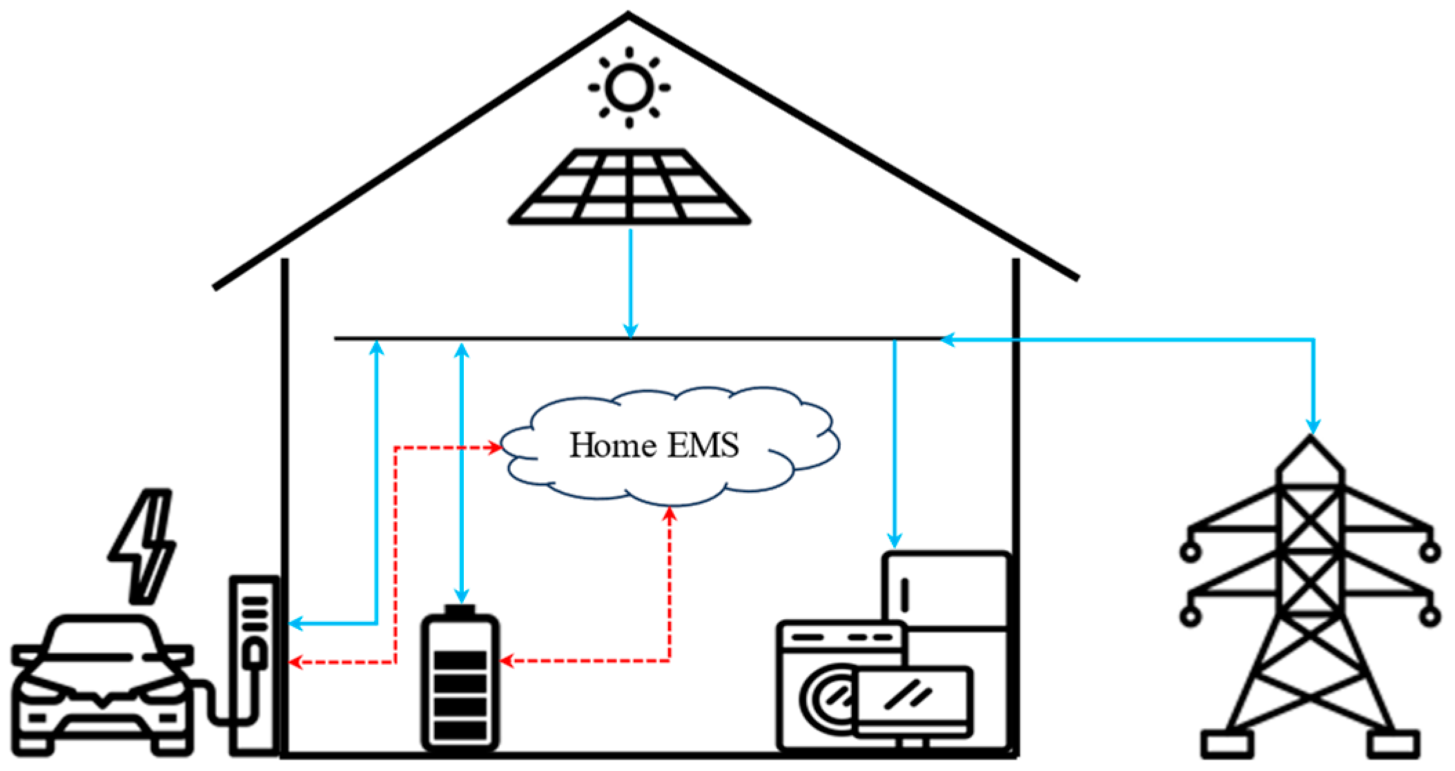
2. EMS Structure and Methodology

The operation planning problem to be solved by the EMS can be stated as follows:

Given the following:

• The PV panels, the EV charging station, and the BESS installed in the household with their size/capacity, and technical operational limits;
• The day-ahead hourly forecast and real-time measurements of residential consumption, ${\overline{Load}}_t^{fore}$ and ${\overline{Load}}_t^{real}$;
• The day-ahead hourly forecast and real-time measurements of PV production, ${\overline{PV}}_t^{fore}$ and ${\overline{PV}}_t^{real}$;
• The forecast of electricity purchase and selling price profiles, ${\overline{c}}_t^{purch},{\overline{r}}_t^{sell}$;
• The day-ahead forecast schedule of the electric vehicle usage (in particular, the time periods t in which the EV is at used, ${\overline{Avail}}_{ev,t}$ = 0, and the expected energy consumption for the trip, ${\overline{Demand}}_{ev,t}$).

Determine the optimal planning of controllable components (BESS and EV), i.e., the battery charge/discharge profile, $P_{es,t}^{net}$, and the electric vehicle charge/discharge profile, $P_{ev,t}^{net}$, which minimize the total operational cost for the house.

The operational planning solution must meet the following constraints:

• The storage operational constraints;
• The maximum grid import and export limitation;
• The power balance of the house;
• The achievement of a minimum state of charge (SOC) of the EV battery at the time requested by the user.

The scheme of the developed home energy management system (HEMS) is shown in Figure 2. It follows a rolling-horizon approach: a time-dependent model is solved repeatedly, and its planning interval is moved forward in time. It consists of two layers: the first layer solves a predictive optimization problem over a time horizon of 24 h with a time discretization of 1 h, while the second layer controls the instantaneous power balance. The second layer adjusts the BESS and the EV charge/discharge power to compensate for the errors in the forecasts of PV power production and load demands.

The control structure for the second layer adopts a heuristic model that mitigates deviations between forecasts and actual outcomes. The heuristic model acts on each step of the first-layer models with a time discretization of 15 min. It is noteworthy that the heuristic model computational time is very short, allowing for potential frequency increases, even down to seconds. However, the frequency of the second layer aligns with the measurements provided by Edison, which are associated with second-generation smart meters collecting data every 15 min.

2.1. Forecasting Module

The forecasting module supplies the home EMS with input profiles necessary for predictive optimization, enabling strategic planning for system components. As shown in Figure 2, these forecasted profiles are the house consumption, PV generation, electricity prices (purchase and selling prices), EV time of usage (i.e., time periods in which the EV is not connected to the charging station), and energy consumption of the EV in the travels.

The PV generation and the house consumption forecasts deliver predictions for the upcoming day at its initiation. These predictions are developed by Edison, and they are detailed in Section 3.2 and Section 3.3.

As far as electricity prices for Italian domestic clients are concerned, the selling price follows the “Ritiro Dedicato” [34] scheme, where electricity injected into the grid is sold at the zonal price, “Prezzo Zonale” (PZ). Regarding the purchase price, due to transport costs and taxes, it is about twice the market clearing price, known as “Prezzo Unico Nazionale” (PUN) in Italy. It is worth noting that PZ and PUN are typically quite similar, differing only when market splitting occurs in the day-ahead market (DAM) resolution [35], particularly in the north bidding zone. In normal socio-economic conditions, the PUN (thus the electricity selling and purchasing prices) can be day-ahead forecasted with 15–20% mean absolute percentage error (MAPE) error [36] using support vector machine algorithms. However, during the EMS testing period, which ranges from 28 January 2022 until 28 January 2023, electricity prices were very volatile as a consequence of geopolitical tensions, when minimums around 20 €/MWh and peaks up to 870 €/MWh were recorded (see Figure 3). Therefore, instead of developing a forecasting module, historical data for purchase and selling prices have been considered, which were available from [37]. Future testing activities of the EMS, hopefully in stable geo-political periods, will also include the price forecast module.

As for the EV, unfortunately, the number of clients with EV is insufficient to derive a consistent methodology for forecasting EV usage (availability time and consumed energy). Thus, the EMS has been tested assuming a set of four different EVs’ expected usage profiles, as detailed in Section 3.5. Additionally, the economic impact of EV usage forecast errors has been assessed for different error scenarios for both a winter week and a summer week, as discussed in Section 4.7.

2.2. First Layer—MILP Mathematical Formulation

The first layer of the home EMS is designed as a deterministic MILP, where all operational variables and constraints are defined for each timestep. The variables used in this work are listed and described in the nomenclature section.

The decision variables in the optimization problem include the following:

• Battery storage: average charging power $P_{es,t}^{ch}$, discharging power $P_{es,t}^{disch}$, net power exchange $P_{es,t}^{net}$, and state-of-energy ${SOE}_{es,t}$ for each timestep t;
• Electric vehicle: average charging power $P_{ev,t}^{ch}$, discharging power $P_{ev,t}^{disch}$, net power exchange $P_{ev,t}^{net}$, and state-of-energy ${SOE}_{ev,t}$ for each timestep t;
• Grid interaction: average power purchased from the grid $P_t^{grid,purch}$ and power sold back to the grid $P_t^{grid,sell}$ for each timestep t.

Since the time horizon is discretized, the power-related operational variables (e.g., $P_{es,t}^{disch}$ as kW) are considered timestep-averaged values. The corresponding energy quantities are obtained by multiplying the power values by the timestep duration ${\overline{dt}}_1$. For instance, if the timestep duration is one hour, then the numerical values for average power and energy remain identical.

The optimization problem focuses on defining the household’s strategic planning and economic dispatch by minimizing total operational costs, expressed as follows:

$$OF=min\left(\sum _{t \in T_1}{\mathsf{\Phi }}_t^{Opex}\right)$$

(1)

The key constraints governing the model include the following:

• Storage dynamics: for both the battery and the EV, constraints define charging and discharging power limits as well as the state-of-charge evolution over time;
• Grid constraints: electricity purchased and sold must comply with the contractual limits of the user;
• Power balance: at each timestep, the total electricity generated by non-dispatchable sources, energy discharged from storage, and energy purchased from the grid must always balance the total energy used for storage charging and exports to the grid.

For brevity, the complete MILP mathematical model is not provided here. The developed model, encompassing constraints and the objective function, adheres to the deterministic formulations proposed by Thomas et al. [24] and Melhem et al. [38].

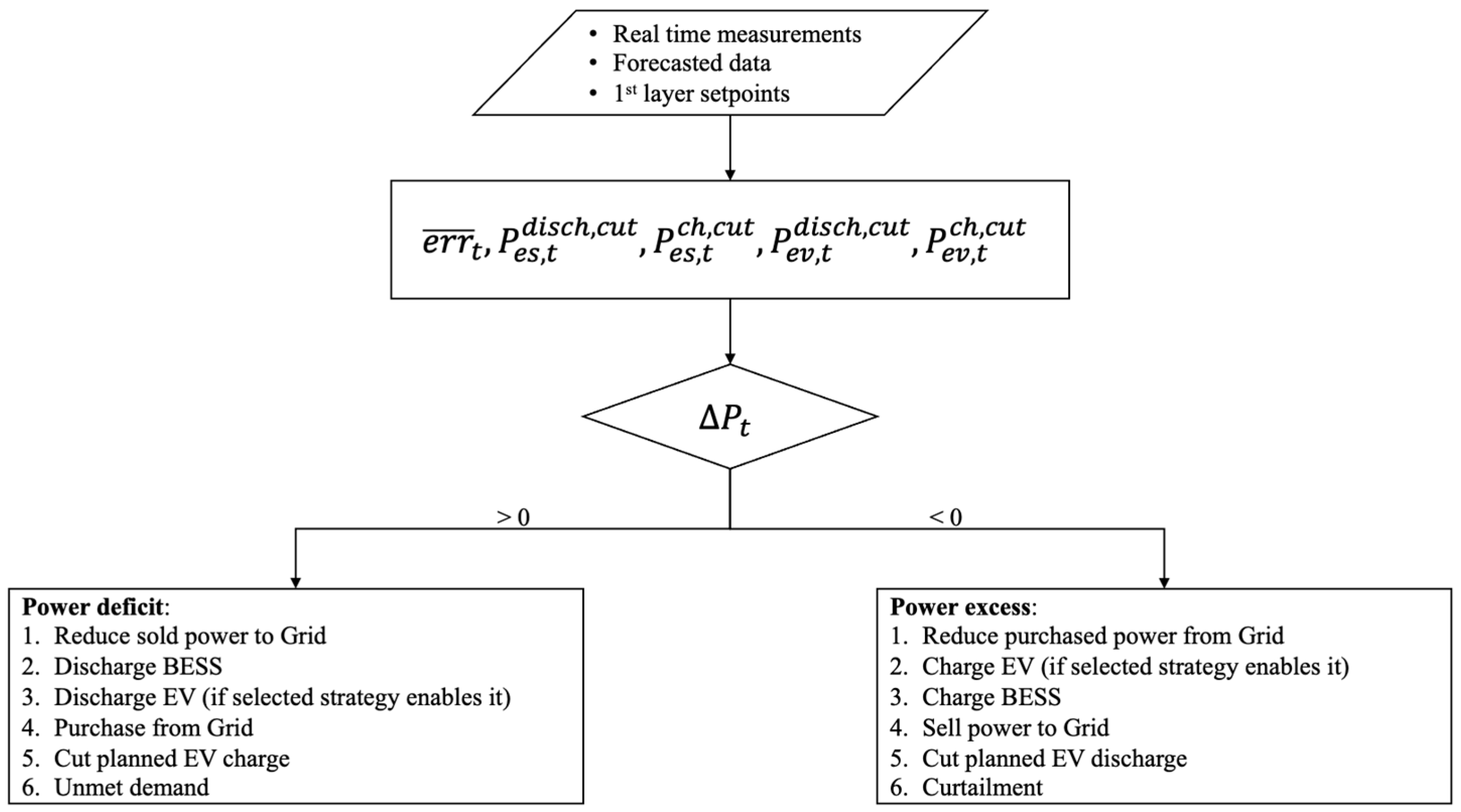
2.3. Second Layer—Heuristic Control

The second layer of the home EMS is a rule-based control algorithm that refines the optimal setpoints obtained from the first-layer MILP model. Its primary function is to manage the net demand forecast error—caused by inaccuracies in predicting PV generation and household consumption—by redistributing this error among system components while respecting their technical limitations. This layer dynamically adjusts power setpoints based on real-time system measurements, ensuring an effective interaction between the BESS and the EV in maintaining home energy balance.

The net demand forecast error can be computed as follows:

$${\overline{err}}_t={\overline{Load}}_t^{real}-{\overline{Load}}_t^{fore}-\left({\overline{PV}}_t^{real}-{\overline{PV}}_t^{fore}\right) \hspace{1em} \hspace{1em} \hspace{1em} \hspace{1em} \hspace{1em} \hspace{1em} \hspace{1em} \hspace{1em} \hspace{1em} \hspace{1em} \hspace{1em} \hspace{1em} \hspace{1em} \hspace{1em} \hspace{1em} \hspace{1em} \hspace{1em} \forall t\in T_2$$

(2)

Additionally, at each timestep, adjustments must be made to the EV and BESS power setpoints to account for situations where technical constraints prevent their full execution. This is reflected in the planned state-of-energy (SOE) evolution for the BESS and EV:

$${SOE}_{es,t}^{plan}={SOE}_{es,t-1}·{\overline{\eta }}_{es}^{SD}+(P_{es,t}^{ch,setpoint}·{\overline{\eta }}_{es}^{ch}-{\displaystyle \raisebox{1ex}{$P_{es,t}^{disch,setpoint}$}\!\left/ \!\raisebox{-1ex}{${\overline{\eta }}_{es}^{disch}$}\right.})·{\overline{dt}}_2 \hspace{1em} \hspace{1em} \hspace{1em} \hspace{1em} \hspace{1em} \hspace{1em} \hspace{1em} \hspace{1em} \hspace{1em} \forall t\in T_2$$

(3)

$${SOE}_{ev,t}^{plan}={SOE}_{ev,t-1}·{\overline{\eta }}_{ev}^{SD}+(P_{ev,t}^{ch,setpoint}·{\overline{\eta }}_{ev}^{ch}-{\displaystyle \raisebox{1ex}{$P_{ev,t}^{disch,setpoint}$}\!\left/ \!\raisebox{-1ex}{${\overline{\eta }}_{ev}^{disch}$}\right.})·{\overline{dt}}_2 \hspace{1em} \hspace{1em} \hspace{1em} \hspace{1em} \hspace{1em} \hspace{1em} \hspace{1em} \hspace{1em} \hspace{1em} \hspace{1em}\forall t\in T_2$$

(4)

If these planned SOE values violate operational limits, power setpoints are adjusted accordingly:

$$P_{es,t}^{disch,cut}=min\left\{P_{es,t}^{disch, setpoint}, max\left\{{\overline{\eta }}_{es}^{disch}·{\displaystyle \frac{{\overline{SOE}}_{es}^{min}-{SOE}_{es,t}^{plan}}{{\overline{dt}}_2}},0\right\}\right\} \hspace{1em} \hspace{1em} \hspace{1em} \hspace{1em} \hspace{1em} \hspace{1em} \hspace{1em} \hspace{1em} \hspace{1em} \hspace{1em} \hspace{1em} \forall t\in T_2$$

(5)

$$P_{es,t}^{ch,cut}=min\left\{P_{es,t}^{ch, setpoint}, max\left\{{\displaystyle \frac{{SOE}_{es,t}^{plan}-{\overline{SOE}}_{es}^{min}}{{\overline{\eta }}_{es}^{ch}·{\overline{dt}}_2}},0\right\}\right\} \hspace{1em} \hspace{1em} \hspace{1em} \hspace{1em} \hspace{1em} \hspace{1em} \hspace{1em} \hspace{1em} \hspace{1em} \hspace{1em} \hspace{1em} \hspace{1em} \hspace{1em} \hspace{1em} \hspace{1em}\forall t\in T_2$$

(6)

$$P_{ev,t}^{disch,cut}=min\left\{P_{ev,t}^{disch, setpoint}, max\left\{{\overline{\eta }}_{ev}^{disch}·{\displaystyle \frac{{\overline{SOE}}_{ev}^{min}-{SOE}_{ev,t}^{plan}}{{\overline{dt}}_2}},0\right\}\right\} \hspace{1em} \hspace{1em} \hspace{1em} \hspace{1em} \hspace{1em} \hspace{1em} \hspace{1em} \hspace{1em} \hspace{1em} \hspace{1em}\hspace{1em} \forall t\in T_2$$

(7)

$$P_{ev,t}^{ch,cut}=min\left\{P_{ev,t}^{ch, setpoint}, max\left\{{\displaystyle \frac{{SOE}_{ev,t}^{plan}-{\overline{SOE}}_{ev}^{min}}{{\overline{\eta }}_{ev}^{ch}·{\overline{dt}}_2}},0\right\}\right\} \hspace{1em} \hspace{1em} \hspace{1em} \hspace{1em} \hspace{1em} \hspace{1em} \hspace{1em} \hspace{1em} \hspace{1em} \hspace{1em}\hspace{1em} \hspace{1em}\hspace{1em} \hspace{1em} \hspace{1em} \forall t\in T_2$$

(8)

The computed ${SOE}_{es,t}^{plan}$ and ${SOE}_{ev,t}^{plan}$, shown in Equations (3) and (4), determined at the beginning of this second layer, represent the expected energy levels of the BESS and EV if they were to fully adhere to the first-layer setpoints. The adjustments in power setpoints, Equations (5)–(8), ensure compliance with technical constraints and the optimization strategy.

The total power imbalance to be managed in the second layer is then given by the following:

$${\Delta P}_t={\overline{err}}_t+\left(P_{es,t}^{disch,cut}+P_{ev,t}^{disch,cut}\right)-\left(P_{es,t}^{ch,cut}+P_{ev,t}^{ch,cut}\right) \hspace{1em} \hspace{1em} \hspace{1em} \hspace{1em} \hspace{1em} \hspace{1em} \hspace{1em} \hspace{1em} \hspace{1em} \hspace{1em} \hspace{1em} \hspace{1em} \hspace{1em} \hspace{1em}\forall t\in T_2$$

(9)

Depending on whether ${\Delta P}_t$ is positive or negative, the system must address either a power deficit or a power surplus. Figure 4 presents a block-flow diagram of the second-layer heuristic strategy, detailing the priority order for managing these scenarios:

• Reduce grid interaction;
• BESS or EV power supply (different priority according to power deficit/excess and selected strategy);
• Increase grid interaction;
• Additional cut of planned EV setpoint;
• Unmet demand or curtailment.

In this work, two EV management strategies have been implemented: unidirectional smart charging (V1H) and bidirectional smart charging, also known as vehicle-to-home (V2H). In the second layer of the V1H mode, the EV is charged in the case of power excess taking priority over the BESS, and it is not discharged to cover the power deficit. In the V2H mode, the EV is discharged, giving priority to the BESS. Moreover, the EV discharge in the second layer is enabled only if the residential consumption exceeds the user’s power connection limits.

2.4. Benchmark Algorithm

It is necessary to define a benchmark algorithm to properly assess the HEMS performances from operative and economic perspectives. Since the HEMS relies on predictive optimization, the benchmark algorithm is designed as a non-predictive heuristic control. Boynuegri et al. [39] proposed a heuristic approach to residential environment management, outlining various priority orders among house components to enhance renewable self-consumption. In this study, the benchmark algorithm is similar but with different priority orders according to the EV availability and the net power consumption of the house (computed as the difference between the measured house consumption and PV production). The logic of the benchmark algorithm is depicted in Figure 5. The goal is to replicate the priorities observed in the second layer heuristic control and model the EV charging process to resemble current charging stations. In this context, the EV is charged as rapidly as possible to reach a minimum SOE close to its maximum capacity while adhering to the technical limitations of the system.

3. Case Studies

In this section, the case studies to which the aforementioned methodology is applied are presented.

Each case study differs in terms of users’ weekly commuting habits (ranging from no remote working days to three days per week). A reference case has also been included, denoted as case 0, in order to address scenarios with no electric mobility. Assessing this simpler design is essential for understanding the impact of increasing system complexity in terms of components and management strategies. Additionally, this case offers a reference point for calculating the costs and revenues associated with the annual energy consumption of various users in the analyzed configurations, facilitating the computation of the electric mobility effect in subsequent cases. Each case study aims to assess the techno-economic performance of six users in various smart home configurations. The objective is to evaluate the benefits offered by the proposed HEMS in comparison to a benchmark heuristic algorithm.

The analyzed configurations of the smart home environment depend on factors such as the size of the PV system, which varies based on whether the user has low or high annual energy consumption, as well as the presence or absence of BESS and the EV management in V1H or V2H mode. Test cases are summarized in

Table 1. Analyzed configurations according to the user’s annual energy consumption.

User	<3 MWh/y												>3 MWh/y
PV size	No PV = 0 kW				Low PV = 3 kW				High PV = 4.5 kW				No PV = 0 kW				Low PV = 4.5 kW				High PV = 6 kW
BESS	No		Yes		No		Yes		No		Yes		No		Yes		No		Yes		No		Yes
EV	V1H	V2H	V1H	V2H	V1H	V2H	V1H	V2H	V1H	V2H	V1H	V2H	V1H	V2H	V1H	V2H	V1H	V2H	V1H	V2H	V1H	V2H	V1H	V2H

.

The simulations have all been performed on a 1-year period, ranging from 28 January 2022 until 28 January 2023. The considered customers are located in the north of Italy. Overall, 396 instances have been evaluated.

The EMS has been coded in Pyomo (v6.4) [40,41], an open-source Python-based optimization modeling framework that supports a variety of optimization techniques. The first-layer MILP problem is solved using Gurobi Optimizer (v9.5.2) [42]. All optimization simulations have been executed on a workstation equipped with a 3.2 GHz 10-core Apple M1 Pro processor and 16 GB of RAM.

3.1. Key Performance Indicators

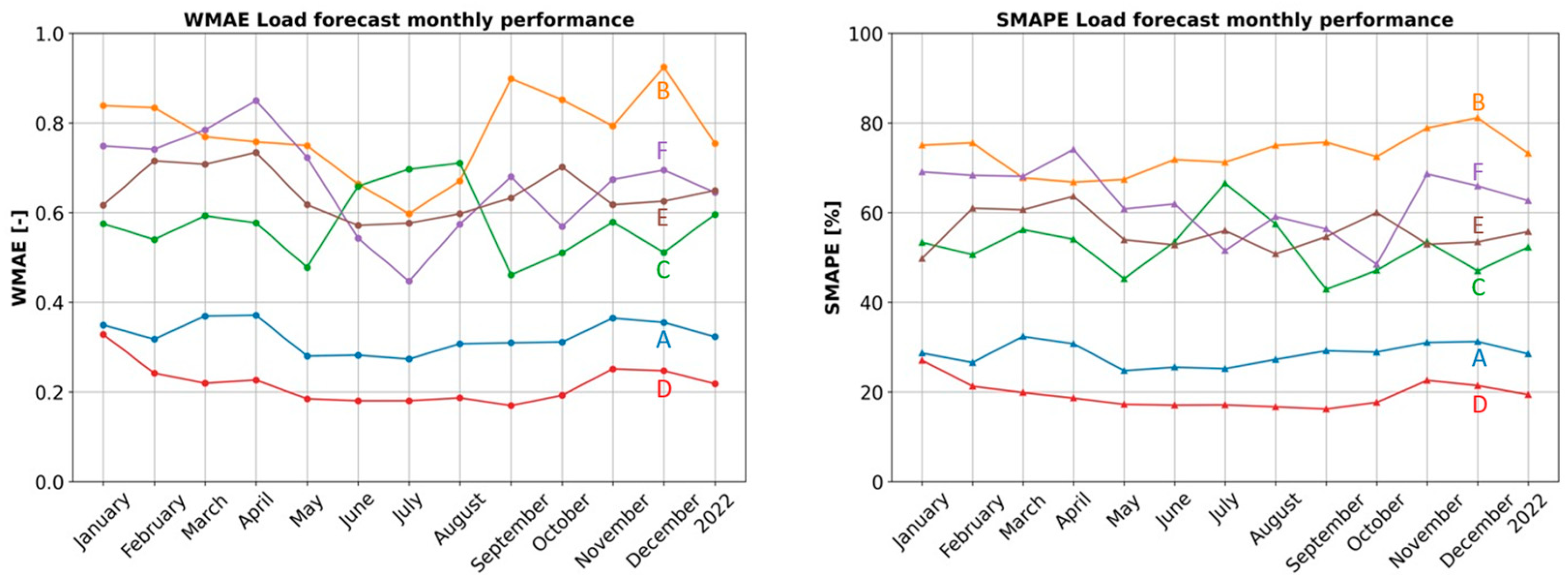
3.1.1. Forecast Module Characterization

To comprehensively evaluate the home EMS, it is necessary to introduce and characterize the inputs that drive its performance since these inputs wield a significant influence. Specifically, quantifying errors linked to the forecast module is crucial. In this study, the assessment utilizes the symmetric mean absolute percentage error (SMAPE) and the weighted mean absolute error (WMAE) to gauge the accuracy of the forecasts.

$$SMAPE[\%]={\displaystyle \frac{100}{n}}{\displaystyle \sum _{i=1}^n}{\displaystyle \frac{\left|y_i-{\widehat{y}}_i\right|}{\left(y_i+{\widehat{y}}_i\right)/2}}$$

(10)

$$WMAE[-]={\displaystyle \frac{{\sum }_{i=1}^n\left|y_i-{\widehat{y}}_i\right|}{{\sum }_{i=1}^n{y}_i}}$$

(11)

where ${\widehat{y}}_i$ is the forecast and $y_i$ is the measurement. These metrics are commonly used to evaluate the accuracy of forecasting models. SMAPE calculates the percentage difference between forecasted and actual values and normalizes it by their mean. It is symmetric, meaning it does not favor overestimations or underestimations. On the other hand, WMAE assesses the average absolute error between forecasted and actual values, with a weighting based on the energy observed throughout the simulation period. This allows for assigning less importance to errors occurring at lower power levels.

3.1.2. Techno-Economic Assessment

The techno-economic performance has been assessed by defining key performance indicators (KPIs) that compare the total costs (TC) of the predictive home EMS with those of the benchmark algorithm. The objective is to quantify the benefits in absolutes (e.g., total costs [€/y]) and relative terms (e.g., annual percentage savings [%]). Relative indicators will be referred to as relative savings (RS), and they can be evaluated for the predictive EMS in either V1H or V2H mode, using the benchmark algorithm as a reference. It is important to clarify that the total costs considered in these KPIs have been adjusted to exclude the operational costs of EV and BESS, focusing solely on the purchase and injection of power into the grid for the economic analysis.

$${RS}_{EMS}={\displaystyle \frac{{TC}_{bench}-{TC}_{EMS}}{\left|{TC}_{bench}\right|}}$$

(12)

The absolute value is used in the denominator to prevent sign changes caused by scenarios that generate annual revenues.

Another noteworthy metric pertains to the cost-effectiveness of adding the stationary BESS. This cost-effectiveness has been assessed using the break-even cost (BEC), which is determined by the operational savings generated by the BESS. The BEC represents the maximum price at which it would be advisable to invest in the installation of the BESS. Below this threshold, there is a net gain, while exceeding it results in a financial loss. Calculating the BEC involves the use of the capital recovery factor (CRF), a ratio for assessing the present value of an annuity (assuming a series of equal annual cash flows). CRF depends on the real discount rate and the BESS lifetime, which are specified in Section 3.4.

$${CRF}_{BESS}={\displaystyle \frac{i·{\left(1+i\right)}^{N_{BESS}}}{{\left(1+i\right)}^{N_{BESS}}-1}}$$

(13)

$${BEC}_{EMS}={\displaystyle \frac{{TC}_{EMS}^{NO BESS}-{TC}_{EMS}^{YES BESS}}{{CRF}_{BESS}}}$$

(14)

In addition to evaluating the economic feasibility of the different configurations for each case study, it is necessary to quantify the self-consumption of PV generation as well. Given that grid power injection has been constrained to the net power excess between residential consumption and PV generation, BESS and EV cannot be discharged to sell electricity to the grid. This implies that PV self-consumption can be easily derived from the difference between the energy generated with PV and the electricity injected into the grid:

$$PV self consumption\left[\%\right]={\displaystyle \frac{{PV}_{self cons}}{{PV}_{prod}}}={\displaystyle \frac{{PV}_{prod}-{Grid}_{sold}}{{PV}_{prod}}}$$

(15)

3.2. PV Production

Edison provided data concerning the PV production forecast and measurements, referencing a PV field situated in the north of Italy. Both forecasts and measurements have been rescaled to a nominal power consistent with the typical size of PV fields in Italian households, following [43]. In Figure 6, the monthly forecast performance is evaluated in terms of SMAPE and WMAE. As depicted, the SMAPE hovers around 30%, and the WMAE is around 0.2, with the lowest performance observed in the months of December and January.

3.3. Residential Consumption

Edison also supplied data on the forecast and measurements of residential consumption for six different users located in the north of Italy. The selection of these users aimed for geographical consistency with the PV field’s location. Furthermore, they were chosen based on their annual energy consumption over the analyzed period to represent statistically significant cases among potential users. The forecast performance for each user’s residential consumption is assessed in terms of WMAE and SMAPE, as illustrated in Figure 7. The errors exhibit strong dependence on the individual user, and no correlations with annual energy consumption were identified. Unfortunately, due to privacy considerations, details regarding household composition—such as the adopted heating system, cooking system, air conditioning, or number of people—are not available. Such information could have enhanced consumption forecasts. Despite these challenges, the suboptimal forecast performances provide valuable insights into the economic impacts of inaccuracies in the home EMS.

Table 2. Users’ characterization and grouping.

	User	Annual Energy Consumption [MWh/y]	WMAE [-]	SMAPE [%]
Low consumption	A	2.23	0.32	28.5%
	B	2.55	0.75	73.2%
	C	2.63	0.6	52.3%
High consumption	D	3.43	0.22	19.4%
	E	3.56	0.65	55.7%
	F	3.85	0.65	62.6%

presents characteristics of the analyzed users, including annual consumption and forecast errors over the entire simulation period. Additionally, a nomenclature introduced for results presentation and grouping by annual energy consumption, as specified in Table 2, will be employed throughout the discussion.

3.4. Techno-Economic Parameters

Table 3. Techno-economic parameters.

	Battery	Nissan Leaf	Tesla Model S
${\overline{size}}_i$	5 kWh	40 kWh	100 kWh
On-road specific consumption	-	0.200 kWh/km	0.270 kWh/km
Nominal charge/discharge power	4.6 kW	7.4 kW	7.4 kW
Charge/discharge efficiency	94%	97%	97%
Self-discharge	0.05%/h	0%/h	0%/h
${\overline{SOC}}_i^{max}$	80%	90%	90%
${\overline{SOC}}_i^{min}$	20%	40%	40%
Throughput cost	30 €/MWh	40 €/MWh	40 €/MWh
$N_{BESS}$ (BESS lifetime)	10 y	-	-
$i$ (discount rate)	8%	-	-

provides an overview of the techno-economic parameters for the main components used in the study. It is worth mentioning that the Nissan Leaf has been utilized in all case studies, while the Tesla Model S has been introduced only in an additional case study with 2 days of remote working. This addition allows for the exploration of the impact of an EV with a larger capacity. To ensure consistency and prevent unmet demand, a grid contract limit of 6 kW has been applied. This decision has been made to maintain accurate economic assessments, as unmet demand economic valuation would require making certain assumptions. Technical parameters regarding BESS and EV efficiencies have been provided by Edison. The charge/discharge efficiency for EV operations has been assumed based on a wired EV charger rather than a wireless one. For more insights into the differences between these technologies, readers are referred to the work of Niu et al. [44].

3.5. EV Weekly Commute

As mentioned earlier, four distinct case studies for EV weekly commuting patterns have been examined for each user. The objective is to assess the influence of varied EV usage on both the weekly availability for the home EMS and the additional load introduced by EV charging needs, closely tied to the yearly mileage. These case studies are summarized in

Table 4. EV weekly commute case studies.

	Yearly Mileage [km]	Days of Remote Working Per Week	Monday	Tuesday	Wednesday	Thursday	Friday	Saturday	Sunday
Case 1	19,986	0	W	W	W	W	W	L	H
Case 2	17,386	1	RW	W	W	W	W	L	H
Case 3	14,630	2	W	RW	W	RW	W	L	H
Case 4	10,556	3	RW	W	RW	W	RW	L	H

W: working day, RW: remote working day, L: EV used for leisure, H: home (no EV usage).

, and the detailed weekly schedules outlining hourly activities can be found in Appendix A. Various levels of remote working have been explored, ranging from no remote working days in Case 1 to up to three days in Case 4. The parameters ${\overline{Demand}}_{ev,t}$ and ${\overline{Avail}}_{ev,t}$ introduce the EV weekly commute in the home EMS.

4. Results and Discussion

In this section, the performance of the home EMS is evaluated against the non-predictive heuristic benchmark algorithm in terms of household components management and economic outcomes. KPIs presented in Section 3.1.2 are reported in Appendix B.

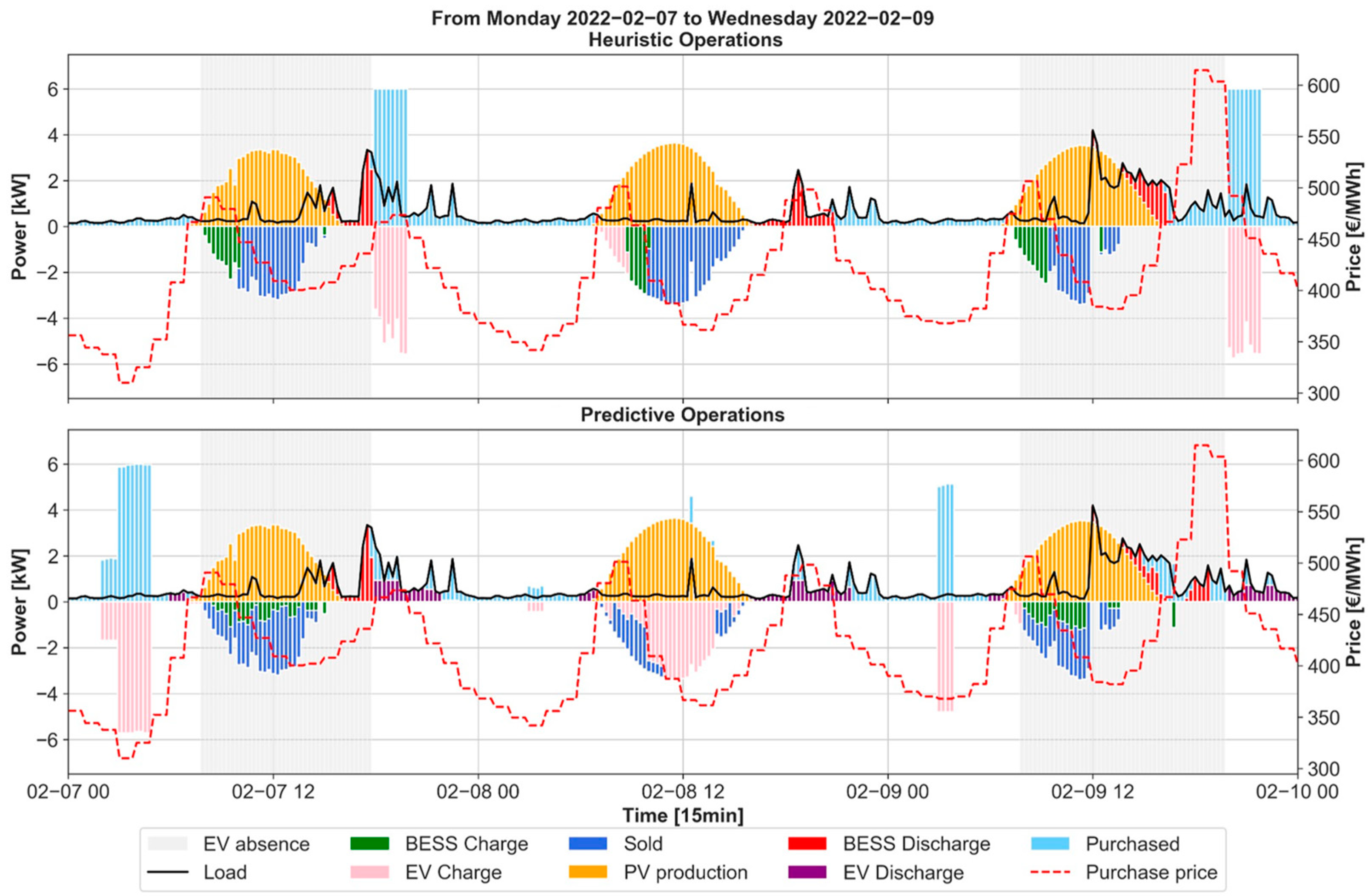
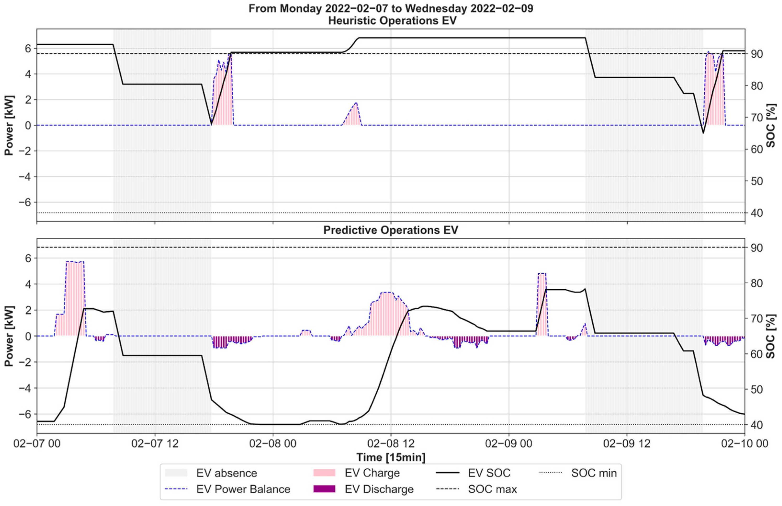
4.1. Predictive vs. Heuristic Management

Before detailing the economic comparison between the home EMS and the non-predictive heuristic benchmark, it is crucial to highlight how these strategies manage household components. This comparison is presented through Figure 7, Figure 8 and Figure 9, where the analysis spans three consecutive days, from Monday, 7 February, to 9 February 2022. As can be noticed from the light gray background indicating the absence of the EV from the house, the considered timeframe includes two working days with a remote working day in between. The operations are specific to user F, possessing a PV nominal size of 6 kW with the capability of performing V2H, but outcomes can be extended to all the analyzed users.

Referring to Figure 8, it is possible to emphasize the distinctions between the strategies in terms of power balance. Firstly, the heuristic strategy charges the EV at the most expensive time of the day when the user returns home. As a non-predictive approach, it cannot leverage information about the upcoming remote working day or take advantage of lower overnight electricity prices. In contrast, the home EMS can opt to charge the EV overnight, capitalizing on lower prices, or postpone the charging to the remote working day when excess PV production is available. Another noteworthy aspect is the examination of peaks in residential consumption. While the heuristic benchmark maximizes the use of the BESS charged with PV excess, the home EMS optimally employs a combination of BESS and EV to minimize grid power purchases during peak expensive hours. This optimization is evident not only in the evening but also in the early morning when the EV is charged overnight and discharged during the early morning price peak before PV production begins. Furthermore, during the remote working day, the home EMS predominantly stores PV excess in the EV and does not consider the BESS. This decision is influenced by the redundancy of having two storage units and contributes to the determination of the economic inefficiency of installing a stationary battery, a point that will be further elaborated in the economic performance analysis.

Figure 9 highlights the differences in EV management. The SOC reduction during its absence is attributed to on-road consumption, and it is assumed that the EV is not charged outside the house. The behavior shown in the upper part of the figure reflects the typical approach seen in current EV charging stations, where the EV is charged to its maximum as quickly as possible, without considering the actual daily usage needs of the EV. In contrast, the home EMS not only charges the EV to meet its daily commute requirements and avoid falling below the minimum SOC of 40% but also strategically charges to supply power during peak hours, leveraging bidirectionality.

The management of the BESS, when involved, does not show significant differences between the heuristic benchmark and the home EMS, as shown in Figure 10. However, the figure does confirm the impracticality of utilizing a BESS during a remote working day when the EV is available, keeping the BESS at its minimum SOC to minimize losses associated with self-discharge.

4.2. Case 0—Reference Without Electric Mobility

This case serves as a reference for a smart home environment without electric mobility. Evaluating the techno-economic performance of this simpler design is essential for understanding the impact of increasing system complexity in terms of components and management strategies. Additionally, this case offers a reference point for calculating the costs and revenues associated with the annual energy consumption of various users in the analyzed configurations, facilitating the computation of electric mobility effect in subsequent cases. Obviously, because of the EV absence, KPIs have been computed only for one mode of the predictive EMS, without distinguishing between V1H and V2H.

As it is possible to see in

Table A5. Total annual operating costs and percentage cost savings (with respect to the benchmark heuristic algorithm) of the tested EMS in the cases of houses with low electricity consumption.

	User	A						B						C
	PV	No		Low		High		No		Low		High		No		Low		High
	BESS	No	Yes	No	Yes	No	Yes	No	Yes	No	Yes	No	Yes	No	Yes	No	Yes	No	Yes
Case 0	${\mathit{T}\mathit{C}}_{\mathit{b}\mathit{e}\mathit{n}\mathit{c}\mathit{h}}$	1372.4	1372.3	−234.0	−469.8	−912.8	−1147.0	1720.7	1720.5	100.2	−154.5	−588.6	−849.5	1749.1	1748.9	112.1	−122.1	−574.7	−812.1
	${\mathit{T}\mathit{C}}_{\mathit{p}\mathit{r}\mathit{e}\mathit{d}}$	1372.4	1229.3	−234.0	−507.7	−912.8	−1184.5	1720.7	1612.1	100.2	−172.6	−588.6	−870.8	1749.1	1631.5	112.1	−142.2	−574.7	−835.2
	${\mathit{R}\mathit{S}}_{\mathit{p}\mathit{r}\mathit{e}\mathit{d}}$	0.0%	10.4%	0.0%	8.1%	0.0%	3.3%	0.0%	6.3%	0.0%	11.7%	0.0%	2.5%	0.0%	6.7%	0.0%	16.5%	0.0%	2.8%
Case 1	${\mathit{T}\mathit{C}}_{\mathit{b}\mathit{e}\mathit{n}\mathit{c}\mathit{h}}$	4246.9	4240.7	2531.1	2235.2	1837.1	1529.5	4588.0	4587.1	2856.7	2556.0	2153.8	1844.2	4615.3	4615.6	2871.2	2570.9	2165.7	1856.2
	${\mathit{T}\mathit{C}}_{\mathit{V}1\mathit{H}}$	3402.5	3273.5	1675.0	1403.2	934.1	658.0	3751.6	3655.5	1990.6	1718.8	1234.7	947.1	3783.1	3679.3	2023.0	1768.0	1267.3	1000.2
	${\mathit{T}\mathit{C}}_{\mathit{V}2\mathit{H}}$	3300.5	3215.8	1579.9	1391.0	836.5	647.4	3643.1	3573.9	1874.1	1673.4	1111.8	904.2	3662.1	3590.2	1904.7	1720.5	1143.4	953.2
	${\mathit{R}\mathit{S}}_{\mathit{V}1\mathit{H}}$	19.9%	22.8%	33.8%	37.2%	49.2%	57.0%	18.2%	20.3%	30.3%	32.8%	42.7%	48.6%	18.0%	20.3%	29.5%	31.2%	41.5%	46.1%
	${\mathit{R}\mathit{S}}_{\mathit{V}2\mathit{H}}$	22.3%	24.2%	37.6%	37.8%	54.5%	57.7%	20.6%	22.1%	34.4%	34.5%	48.4%	51.0%	20.7%	22.2%	33.7%	33.1%	47.2%	48.6%
Case 2	${\mathit{T}\mathit{C}}_{\mathit{b}\mathit{e}\mathit{n}\mathit{c}\mathit{h}}$	3838.6	3836.4	2139.4	1859.7	1451.1	1159.7	4179.8	4180.6	2465.1	2181.0	1764.9	1471.4	4208.3	4207.4	2479.0	2193.3	1779.4	1485.1
	${\mathit{T}\mathit{C}}_{\mathit{V}1\mathit{H}}$	3183.2	3051.6	1448.0	1175.5	709.1	433.1	3532.3	3432.1	1761.4	1492.0	1009.1	722.5	3563.7	3454.9	1787.6	1531.3	1036.1	767.9
	${\mathit{T}\mathit{C}}_{\mathit{V}2\mathit{H}}$	3050.7	2988.3	1331.7	1170.3	593.5	431.7	3385.8	3337.1	1628.6	1454.7	873.1	695.6	3402.4	3352.6	1648.5	1494.3	893.0	733.7
	${\mathit{R}\mathit{S}}_{\mathit{V}1\mathit{H}}$	17.1%	20.5%	32.3%	36.8%	51.1%	62.7%	15.5%	17.9%	28.5%	31.6%	42.8%	50.9%	15.3%	17.9%	27.9%	30.2%	41.8%	48.3%
	${\mathit{R}\mathit{S}}_{\mathit{V}2\mathit{H}}$	20.5%	22.1%	37.8%	37.1%	59.1%	62.8%	19.0%	20.2%	33.9%	33.3%	50.5%	52.7%	19.2%	20.3%	33.5%	31.9%	49.8%	50.6%
Case 3 Nissan Leaf	${\mathit{T}\mathit{C}}_{\mathit{b}\mathit{e}\mathit{n}\mathit{c}\mathit{h}}$	3397.8	3397.4	1694.0	1418.5	1013.6	735.5	3742.4	3741.2	2026.9	1750.7	1337.9	1053.1	3768.1	3769.2	2038.2	1768.5	1348.8	1073.8
	${\mathit{T}\mathit{C}}_{\mathit{V}1\mathit{H}}$	2843.6	2712.1	1044.4	787.8	305.2	40.4	3190.9	3036.1	1350.0	1042.4	597.9	271.6	3224.2	3118.7	1389.0	1154.5	624.8	316.5
	${\mathit{T}\mathit{C}}_{\mathit{V}2\mathit{H}}$	2706.8	2643.3	902.2	774.5	155.5	28.6	2989.6	2915.9	1113.0	951.8	419.6	281.9	3064.7	3011.4	1219.6	1097.7	365.2	210.2
	${\mathit{R}\mathit{S}}_{\mathit{V}1\mathit{H}}$	16.3%	20.2%	38.3%	44.5%	69.9%	94.5%	14.7%	18.8%	33.4%	40.5%	55.3%	74.2%	14.4%	17.3%	31.9%	34.7%	53.7%	70.5%
	${\mathit{R}\mathit{S}}_{\mathit{V}2\mathit{H}}$	20.3%	22.2%	46.7%	45.4%	84.7%	96.1%	20.1%	22.1%	45.1%	45.6%	68.6%	73.2%	18.7%	20.1%	40.2%	37.9%	72.9%	80.4%
Case 3 Tesla Model S	${\mathit{T}\mathit{C}}_{\mathit{b}\mathit{e}\mathit{n}\mathit{c}\mathit{h}}$	4046.5	4046.8	2186.5	1920.0	1501.5	1222.8	4385.5	4385.1	2504.9	2243.4	1810.6	1533.5	4414.7	4414.7	2526.5	2273.8	1831.8	1560.4
	${\mathit{T}\mathit{C}}_{\mathit{V}1\mathit{H}}$	3372.1	3243.7	1534.6	1287.5	789.5	528.2	3721.0	3626.6	1849.0	1610.2	1087.6	816.2	3752.9	3649.8	1881.5	1658.1	1120.2	872.1
	${\mathit{T}\mathit{C}}_{\mathit{V}2\mathit{H}}$	3231.8	3174.8	1397.9	1272.7	640.7	516.0	3571.3	3524.9	1690.3	1562.3	904.9	770.7	3588.6	3540.5	1719.9	1600.0	939.0	815.2
	${\mathit{R}\mathit{S}}_{\mathit{V}1\mathit{H}}$	16.7%	19.8%	29.8%	32.9%	47.4%	56.8%	15.2%	17.3%	26.2%	28.2%	39.9%	46.8%	15.0%	17.3%	25.5%	27.1%	38.8%	44.1%
	${\mathit{R}\mathit{S}}_{\mathit{V}2\mathit{H}}$	20.1%	21.5%	36.1%	33.7%	57.3%	57.8%	18.6%	19.6%	32.5%	30.4%	50.0%	49.7%	18.7%	19.8%	31.9%	29.6%	48.7%	47.8%
Case 4	${\mathit{T}\mathit{C}}_{\mathit{b}\mathit{e}\mathit{n}\mathit{c}\mathit{h}}$	2889.4	2889.6	1202.1	937.7	524.0	259.3	3232.6	3233.4	1539.2	1268.4	848.7	570.9	3262.4	3261.5	1551.1	1280.2	864.2	586.5
	${\mathit{T}\mathit{C}}_{\mathit{V}1\mathit{H}}$	2464.8	2330.5	662.0	412.6	−69.0	−334.7	2814.0	2712.7	977.6	730.5	233.6	−40.4	2845.0	2734.0	1000.3	772.0	259.8	4.0
	${\mathit{T}\mathit{C}}_{\mathit{V}2\mathit{H}}$	2287.2	2254.2	497.6	406.9	−241.2	−331.8	2620.9	2592.9	789.6	688.9	33.0	−69.7	2633.2	2608.3	801.9	722.5	48.0	−33.5
	${\mathit{R}\mathit{S}}_{\mathit{V}1\mathit{H}}$	14.7%	19.3%	44.9%	56.0%	113.2%	229.1%	12.9%	16.1%	36.5%	42.4%	72.5%	107.1%	12.8%	16.2%	35.5%	39.7%	69.9%	99.3%
	${\mathit{R}\mathit{S}}_{\mathit{V}2\mathit{H}}$	20.8%	22.0%	58.6%	56.6%	146.0%	227.9%	18.9%	19.8%	48.7%	45.7%	96.1%	112.2%	19.3%	20.0%	48.3%	43.6%	94.4%	105.7%

and

Table A6. Total annual operating costs and percentage cost savings (with respect to the benchmark heuristic algorithm) of the tested EMS in the cases of houses with high electricity consumption.

	User	D						E						F
	PV	No		Low		High		No		Low		High		No		Low		High
	BESS	No	Yes	No	Yes	No	Yes	No	Yes	No	Yes	No	Yes	No	Yes	No	Yes	No	Yes
Case 0	${\mathit{T}\mathit{C}}_{\mathit{b}\mathit{e}\mathit{n}\mathit{c}\mathit{h}}$	2103.5	2103.3	−303.9	−588.0	−978.3	−1266.6	2146.2	2146.0	−235.3	−516.1	−918.0	−1200.0	2545.2	2545.0	24.6	−229.3	−668.0	−927.4
	${\mathit{T}\mathit{C}}_{\mathit{p}\mathit{r}\mathit{e}\mathit{d}}$	2103.5	1926.2	−303.9	−635.5	−978.3	−1309.7	2146.2	2000.9	−235.3	−547.1	−918.0	−1228.9	2545.2	2426.6	24.6	−260.8	−668.0	−956.6
	${\mathit{R}\mathit{S}}_{\mathit{p}\mathit{r}\mathit{e}\mathit{d}}$	0.0%	8.4%	0.0%	8.1%	0.0%	3.4%	0.0%	6.8%	0.0%	6.0%	0.0%	2.4%	0.0%	4.7%	0.0%	13.7%	0.0%	3.1%
Case 1	${\mathit{T}\mathit{C}}_{\mathit{b}\mathit{e}\mathit{n}\mathit{c}\mathit{h}}$	4971.4	4970.2	2443.0	2144.7	1753.7	1451.7	5008.0	5006.0	2514.0	2202.9	1823.5	1507.7	5405.4	5406.1	2775.0	2488.1	2072.3	1780.7
	${\mathit{T}\mathit{C}}_{\mathit{V}1\mathit{H}}$	4134.3	3972.9	1554.5	1228.6	817.4	488.6	4178.1	4051.8	1625.3	1318.4	881.7	572.0	4577.9	4474.2	1875.8	1587.5	1120.1	824.6
	${\mathit{T}\mathit{C}}_{\mathit{V}2\mathit{H}}$	3969.9	3861.7	1391.7	1176.0	651.8	436.5	4021.7	3934.3	1469.3	1254.8	719.8	506.4	4437.4	4355.4	1729.8	1508.9	969.6	747.6
	${\mathit{R}\mathit{S}}_{\mathit{V}1\mathit{H}}$	16.8%	20.1%	36.4%	42.7%	53.4%	66.3%	16.6%	19.1%	35.4%	40.2%	51.6%	62.1%	15.3%	17.2%	32.4%	36.2%	45.9%	53.7%
	${\mathit{R}\mathit{S}}_{\mathit{V}2\mathit{H}}$	20.1%	22.3%	43.0%	45.2%	62.8%	69.9%	19.7%	21.4%	41.6%	43.0%	60.5%	66.4%	17.9%	19.4%	37.7%	39.4%	53.2%	58.0%
Case 2	${\mathit{T}\mathit{C}}_{\mathit{b}\mathit{e}\mathit{n}\mathit{c}\mathit{h}}$	4560.5	4563.3	2055.7	1760.0	1371.2	1072.9	4600.5	4599.7	2125.5	1816.5	1436.0	1125.4	5000.7	5002.3	2384.5	2106.1	1684.5	1399.3
	${\mathit{T}\mathit{C}}_{\mathit{V}1\mathit{H}}$	3915.1	3750.7	1327.1	999.0	593.1	262.3	3958.9	3827.1	1393.1	1086.5	652.7	339.4	4358.6	4251.3	1644.3	1354.8	890.3	593.0
	${\mathit{T}\mathit{C}}_{\mathit{V}2\mathit{H}}$	3699.6	3620.4	1126.9	941.8	391.5	206.2	3756.0	3693.9	1211.7	1030.0	469.6	288.3	4156.1	4097.8	1473.8	1286.7	722.4	533.4
	${\mathit{R}\mathit{S}}_{\mathit{V}1\mathit{H}}$	14.2%	17.8%	35.4%	43.2%	56.7%	75.6%	13.9%	16.8%	34.5%	40.2%	54.6%	69.8%	12.8%	15.0%	31.0%	35.7%	47.1%	57.6%
	${\mathit{R}\mathit{S}}_{\mathit{V}2\mathit{H}}$	18.9%	20.7%	45.2%	46.5%	71.5%	80.8%	18.4%	19.7%	43.0%	43.3%	67.3%	74.4%	16.9%	18.1%	38.2%	38.9%	57.1%	61.9%
Case 3 Nissan Leaf	${\mathit{T}\mathit{C}}_{\mathit{b}\mathit{e}\mathit{n}\mathit{c}\mathit{h}}$	4125.3	4124.5	1616.6	1337.0	937.4	655.2	4165.1	4164.4	1693.5	1395.0	1009.2	706.5	4562.4	4563.5	1949.8	1688.8	1254.6	989.0
	${\mathit{T}\mathit{C}}_{\mathit{V}1\mathit{H}}$	3575.4	3411.2	923.4	606.2	192.3	−133.6	3619.2	3492.1	986.2	693.3	247.3	−51.6	4016.3	3834.9	1245.6	972.3	493.6	208.4
	${\mathit{T}\mathit{C}}_{\mathit{V}2\mathit{H}}$	3353.6	3273.8	624.3	458.9	−63.9	−211.9	3422.7	3358.4	757.3	613.4	9.0	−133.4	3725.2	3634.7	922.9	740.0	268.2	117.7
	${\mathit{R}\mathit{S}}_{\mathit{V}1\mathit{H}}$	13.3%	17.3%	42.9%	54.7%	79.5%	120.4%	13.1%	16.1%	41.8%	50.3%	75.5%	107.3%	12.0%	16.0%	36.1%	42.4%	60.7%	78.9%
	${\mathit{R}\mathit{S}}_{\mathit{V}2\mathit{H}}$	18.7%	20.6%	61.4%	65.7%	106.8%	132.3%	17.8%	19.4%	55.3%	56.0%	99.1%	118.9%	18.4%	20.4%	52.7%	56.2%	78.6%	88.1%
Case 3 Tesla Model S	${\mathit{T}\mathit{C}}_{\mathit{b}\mathit{e}\mathit{n}\mathit{c}\mathit{h}}$	4767.4	4768.8	2112.7	1816.6	1434.6	1133.0	4806.4	4806.3	2169.9	1877.3	1484.3	1184.6	5205.0	5205.0	2424.7	2157.3	1731.5	1461.9
	${\mathit{T}\mathit{C}}_{\mathit{V}1\mathit{H}}$	4104.3	3944.0	1410.4	1097.7	673.2	352.8	4148.4	4023.8	1473.5	1187.2	729.7	431.6	4548.2	4445.3	1736.5	1466.8	975.9	695.2
	${\mathit{T}\mathit{C}}_{\mathit{V}2\mathit{H}}$	3878.6	3804.9	1163.0	1018.0	417.5	272.1	3947.7	3890.1	1248.9	1104.9	494.8	350.6	4331.9	4275.6	1519.7	1372.3	751.4	601.6
	${\mathit{R}\mathit{S}}_{\mathit{V}1\mathit{H}}$	13.9%	17.3%	33.2%	39.6%	53.1%	68.9%	13.7%	16.3%	32.1%	36.8%	50.8%	63.6%	12.6%	14.6%	28.4%	32.0%	43.6%	52.4%
	${\mathit{R}\mathit{S}}_{\mathit{V}2\mathit{H}}$	18.6%	20.2%	45.0%	44.0%	70.9%	76.0%	17.9%	19.1%	42.4%	41.1%	66.7%	70.4%	16.8%	17.9%	37.3%	36.4%	56.6%	58.8%
Case 4	${\mathit{T}\mathit{C}}_{\mathit{b}\mathit{e}\mathit{n}\mathit{c}\mathit{h}}$	3615.5	3617.4	1131.0	847.9	452.6	165.7	3655.4	3655.3	1198.6	906.0	515.3	220.1	4052.9	4053.0	1459.9	1193.4	766.0	491.3
	${\mathit{T}\mathit{C}}_{\mathit{V}1\mathit{H}}$	3196.4	3028.9	553.0	233.5	−173.7	−499.2	3240.3	3106.3	613.0	319.5	−120.6	−421.2	3640.3	3530.8	861.6	593.3	118.8	−161.8
	${\mathit{T}\mathit{C}}_{\mathit{V}2\mathit{H}}$	2913.6	2867.4	259.9	153.9	−472.8	−578.1	2980.9	2948.6	350.9	252.4	−386.1	−482.5	3361.7	3328.0	613.3	507.6	−129.7	−236.2
	${\mathit{R}\mathit{S}}_{\mathit{V}1\mathit{H}}$	11.6%	16.3%	51.1%	72.5%	138.4%	401.2%	11.4%	15.0%	48.9%	64.7%	123.4%	291.4%	10.2%	12.9%	41.0%	50.3%	84.5%	132.9%
	${\mathit{R}\mathit{S}}_{\mathit{V}2\mathit{H}}$	19.4%	20.7%	77.0%	81.9%	204.5%	448.8%	18.5%	19.3%	70.7%	72.1%	174.9%	319.2%	17.1%	17.9%	58.0%	57.5%	116.9%	148.1%

, the benefits offered by a predictive EMS are null or limited because of the few degrees of freedom available in the reference case. Configurations without BESS lack the ability to leverage any degree of freedom, preventing the storage and utilization of PV energy during more cost-effective periods. This results in no difference between benchmark and EMS solutions. Configurations with BESS do show some economic performance improvements, but these improvements are not enough to justify the investment required for installing stationary BESS. In fact, the comparison between BECs from

Table A7. Break-even costs of adding a stationary battery of the tested EMS in V1H and V2H modes.

	User	A			B			C			D			E			F
	PV	No	Low	High	No	Low	High	No	Low	High	No	Low	High	No	Low	High	No	Low	High
Case 0	${\mathit{B}\mathit{E}\mathit{C}}_{\mathit{p}\mathit{r}\mathit{e}\mathit{d}}$	960.3	1836.6	1823.6	728.6	1830.4	1893.6	789.1	1706.4	1748.0	1189.4	2225.0	2223.8	975.1	2091.9	2086.2	795.6	1915.0	1936.3
Case 1	${\mathit{B}\mathit{E}\mathit{C}}_{\mathit{V}1\mathit{H}}$	865.5	1823.7	1852.3	645.0	1824.0	1930.2	696.5	1710.8	1792.3	1083.0	2186.6	2206.7	847.9	2059.2	2078.0	696.0	1934.3	1982.8
	${\mathit{B}\mathit{E}\mathit{C}}_{\mathit{V}2\mathit{H}}$	568.4	1267.7	1268.6	464.0	1346.5	1393.0	482.3	1235.8	1276.2	726.4	1447.5	1444.4	586.5	1439.1	1431.9	550.2	1482.2	1489.7
Case 2	${\mathit{B}\mathit{E}\mathit{C}}_{\mathit{V}1\mathit{H}}$	883.6	1828.8	1851.8	672.6	1808.0	1922.6	730.5	1720.4	1799.8	1103.3	2201.5	2219.7	884.3	2057.6	2101.8	719.9	1942.0	1995.1
	${\mathit{B}\mathit{E}\mathit{C}}_{\mathit{V}2\mathit{H}}$	418.8	1083.2	1086.1	326.7	1166.9	1190.9	333.7	1035.1	1068.7	531.2	1241.7	1242.8	416.8	1219.2	1216.5	391.4	1255.2	1268.2
Case 3 Nissan Leaf	${\mathit{B}\mathit{E}\mathit{C}}_{\mathit{V}1\mathit{H}}$	882.7	1722.2	1776.9	1038.6	2064.1	2189.2	707.8	1573.9	2068.3	1102.3	2128.8	2187.2	852.6	1965.5	2005.7	1217.2	1833.6	1913.9
	${\mathit{B}\mathit{E}\mathit{C}}_{\mathit{V}2\mathit{H}}$	426.4	856.7	851.8	494.6	1081.6	924.3	357.9	818.0	1040.2	535.5	1109.9	993.6	431.1	965.9	956.0	607.2	1227.5	1010.1
Case 3 Tesla Model S	${\mathit{B}\mathit{E}\mathit{C}}_{\mathit{V}1\mathit{H}}$	862.0	1658.0	1753.1	633.5	1602.7	1821.6	691.8	1498.8	1664.4	1076.1	2098.6	2149.9	836.3	1921.2	2000.0	690.4	1810.0	1883.3
	${\mathit{B}\mathit{E}\mathit{C}}_{\mathit{V}2\mathit{H}}$	382.2	840.5	836.3	311.4	859.2	900.3	322.5	804.7	830.5	494.8	972.7	975.0	386.6	965.9	967.6	378.2	989.2	1005.3
Case 4	${\mathit{B}\mathit{E}\mathit{C}}_{\mathit{V}1\mathit{H}}$	901.2	1673.5	1783.3	679.9	1658.1	1838.8	745.0	1532.0	1716.7	1123.9	2143.8	2184.4	899.0	1969.0	2016.7	734.5	1800.1	1882.3
	${\mathit{B}\mathit{E}\mathit{C}}_{\mathit{V}2\mathit{H}}$	221.6	608.9	607.9	188.2	675.3	689.0	167.4	532.7	546.9	310.1	711.5	706.3	216.6	661.4	646.6	226.6	709.3	714.2
Ideal EMS	${\mathit{B}\mathit{E}\mathit{C}}_{\mathit{V}1\mathit{H}}$	882.7	1722.2	1776.9	649.6	1694.6	1850.1	707.8	1573.9	1696.8	1102.3	2128.8	2187.2	852.6	1965.5	2005.7	708.4	1833.6	1913.9
	${\mathit{B}\mathit{E}\mathit{C}}_{\mathit{V}2\mathit{H}}$	426.4	856.7	851.8	345.9	867.9	924.3	357.9	818.0	849.7	535.5	995.5	993.6	431.1	965.9	956.0	413.9	1003.5	1010.1

and the considered BESS investment cost around 4000€ highlights the impracticality of installing it.

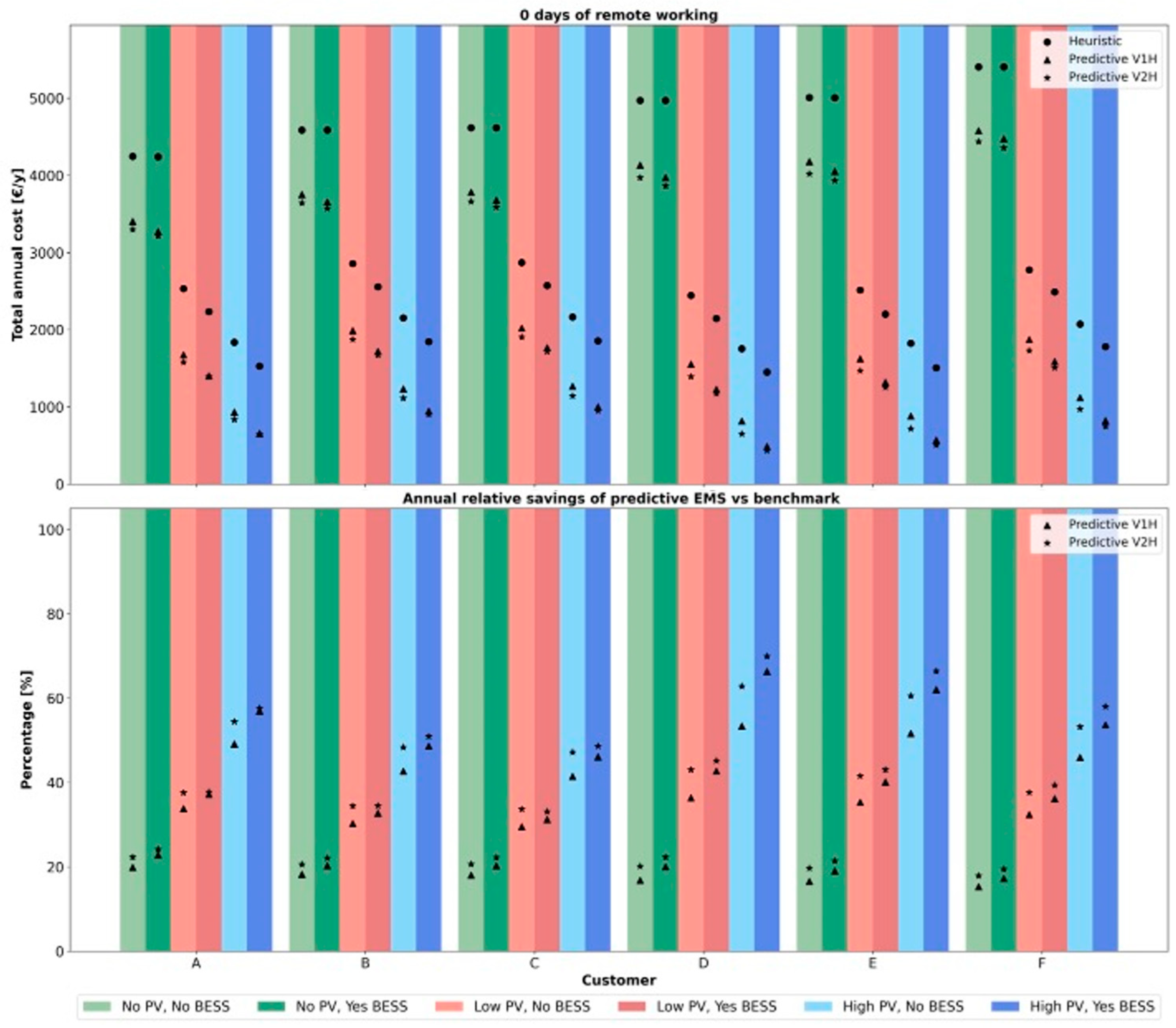
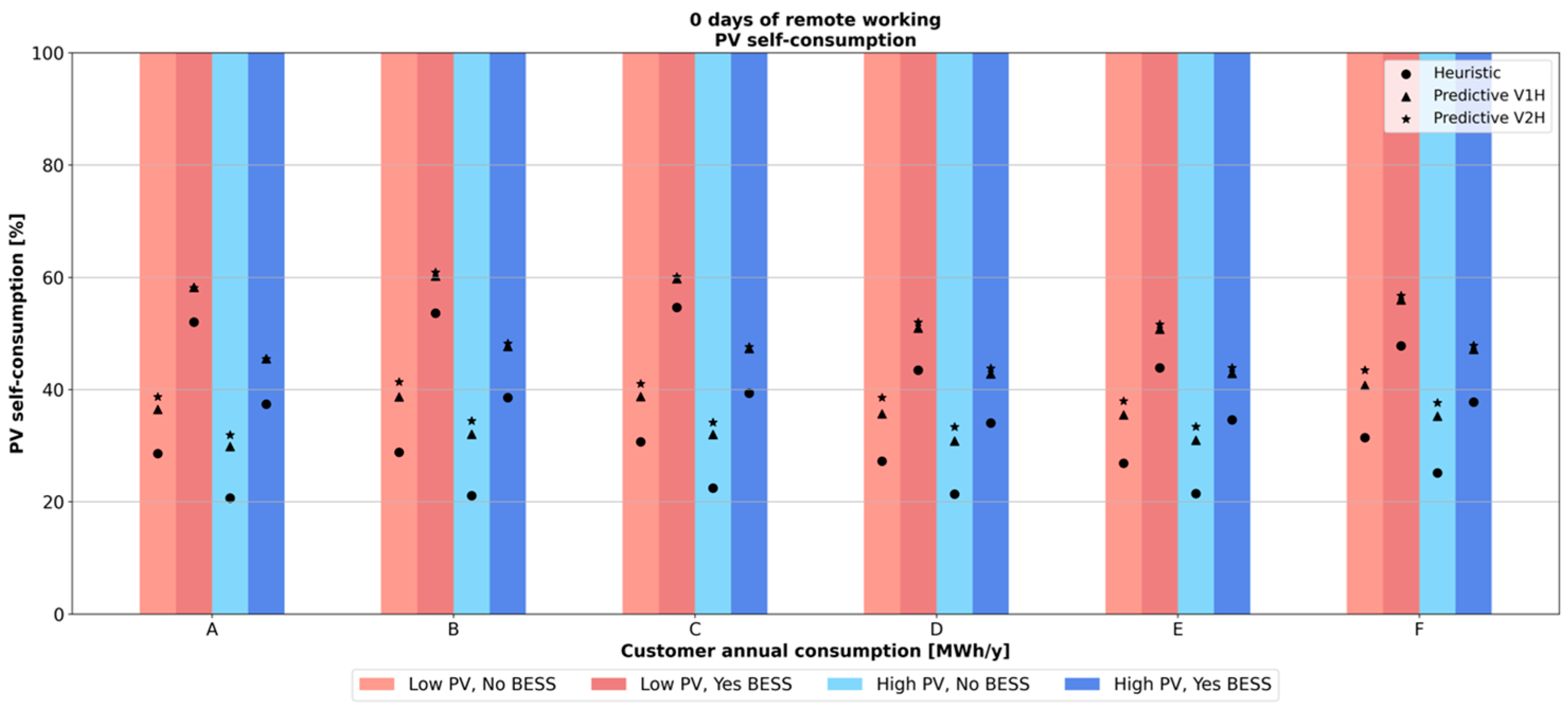
4.3. Case 1—No Days of Remote Working

In this case study electric mobility emerges as an additional load addressed by the home EMS. In addition, it represents the most demanding case study, considering no days of remote working. Figure 11 presents the economic performance results, showcasing total annual costs and annual relative savings for each strategy (heuristic benchmark, home EMS in V1H and V2H modes) in six different configurations for each user, as specified in Table 1. These results are also summarized in Table A5 and Table A6. Following the structure of Figure 11, Figure 12 illustrates the PV self-consumption achieved in each configuration by each strategy, with

Table A8. PV self-consumption (SC) of the tested EMS in cases with installed PV.

	User	A				B				C				D				E				F
	PV	Low		High		Low		High		Low		High		Low		High		Low		High		Low		High
	BESS	No	Yes	No	Yes	No	Yes	No	Yes	No	Yes	No	Yes	No	Yes	No	Yes	No	Yes	No	Yes	No	Yes	No	Yes
Case 1	${\mathit{S}\mathit{C}}_{\mathit{b}\mathit{e}\mathit{n}\mathit{c}\mathit{h}}$	29%	52%	21%	37%	29%	54%	21%	39%	31%	55%	22%	39%	27%	43%	21%	34%	27%	44%	21%	35%	31%	48%	25%	38%
	${\mathit{S}\mathit{C}}_{\mathit{V}1\mathit{H}}$	36%	58%	30%	46%	39%	60%	32%	48%	39%	60%	32%	47%	36%	51%	31%	43%	35%	51%	31%	43%	41%	56%	35%	47%
	${\mathit{S}\mathit{C}}_{\mathit{V}2\mathit{H}}$	39%	58%	32%	45%	41%	61%	34%	48%	41%	60%	34%	48%	39%	52%	33%	44%	38%	52%	33%	44%	43%	57%	38%	48%
Case 2	${\mathit{S}\mathit{C}}_{\mathit{b}\mathit{e}\mathit{n}\mathit{c}\mathit{h}}$	28%	51%	20%	37%	28%	52%	20%	38%	30%	54%	22%	38%	26%	43%	21%	34%	26%	43%	21%	34%	31%	47%	25%	37%
	${\mathit{S}\mathit{C}}_{\mathit{V}1\mathit{H}}$	36%	58%	29%	45%	38%	60%	31%	47%	39%	60%	32%	47%	35%	50%	30%	42%	35%	50%	31%	42%	40%	55%	35%	46%
	${\mathit{S}\mathit{C}}_{\mathit{V}2\mathit{H}}$	41%	57%	33%	44%	43%	60%	35%	47%	44%	60%	35%	47%	41%	52%	35%	44%	40%	52%	35%	43%	45%	56%	38%	47%
Case 3 Nissan Leaf	${\mathit{S}\mathit{C}}_{\mathit{b}\mathit{e}\mathit{n}\mathit{c}\mathit{h}}$	29%	52%	20%	37%	28%	52%	20%	37%	30%	53%	22%	38%	27%	43%	21%	33%	27%	43%	21%	34%	31%	47%	25%	37%
	${\mathit{S}\mathit{C}}_{\mathit{V}1\mathit{H}}$	45%	64%	35%	50%	47%	66%	37%	51%	47%	66%	37%	51%	41%	56%	35%	46%	42%	56%	35%	47%	46%	60%	39%	50%
	${\mathit{S}\mathit{C}}_{\mathit{V}2\mathit{H}}$	51%	64%	41%	49%	55%	68%	43%	52%	54%	66%	44%	53%	50%	59%	41%	48%	49%	58%	42%	48%	53%	62%	44%	51%
Case 3 Tesla Model S	${\mathit{S}\mathit{C}}_{\mathit{b}\mathit{e}\mathit{n}\mathit{c}\mathit{h}}$	40%	62%	28%	44%	41%	62%	29%	45%	42%	62%	30%	45%	35%	50%	27%	39%	35%	51%	28%	40%	40%	55%	31%	43%
	${\mathit{S}\mathit{C}}_{\mathit{V}1\mathit{H}}$	49%	67%	38%	53%	51%	69%	41%	55%	51%	68%	41%	54%	44%	58%	37%	48%	45%	58%	38%	49%	49%	62%	42%	52%
	${\mathit{S}\mathit{C}}_{\mathit{V}2\mathit{H}}$	54%	67%	43%	52%	57%	69%	46%	55%	56%	69%	46%	55%	52%	60%	44%	50%	51%	60%	44%	50%	55%	63%	47%	53%
Case 4	${\mathit{S}\mathit{C}}_{\mathit{b}\mathit{e}\mathit{n}\mathit{c}\mathit{h}}$	28%	50%	19%	35%	27%	50%	20%	36%	29%	52%	21%	37%	26%	42%	20%	33%	26%	42%	20%	33%	30%	46%	24%	36%
	${\mathit{S}\mathit{C}}_{\mathit{V}1\mathit{H}}$	44%	62%	34%	48%	46%	64%	36%	50%	46%	64%	36%	49%	40%	54%	33%	44%	40%	54%	34%	45%	45%	58%	38%	48%
	${\mathit{S}\mathit{C}}_{\mathit{V}2\mathit{H}}$	51%	61%	40%	47%	55%	64%	43%	49%	55%	64%	43%	49%	50%	56%	41%	47%	49%	56%	41%	46%	53%	59%	44%	49%

providing further details on the PV self-consumption results.

Several significant insights can be gleaned from these techno-economic performances. Firstly, when comparing the total annual cost of this case with scenarios without electric mobility, it becomes evident that the additional load introduced by mobility needs is typically more substantial than that associated solely with residential consumption. This significantly increases the overall load that the home must manage. However, EV charging is a programmable load, differing from the non-programmable nature of residential consumption. This flexibility can be harnessed to reduce costs. As shown in Figure 11, the home EMS can achieve noteworthy savings in all analyzed configurations. Even in scenarios without PV production, representing the least flexible conditions, leveraging lower overnight electricity prices for EV charging alone introduces savings of around 20% per year. The introduction of and increase in PV generation further reduce costs and increase savings, reaching over 60% for high consumption users. The additional flexibility provided by bidirectional smart charging enhances economic performance, especially in configurations without BESS, with additional savings of around 5%, enabling the EV to cover residential consumption during price peaks, as discussed in Section 4.1. In configurations with BESS, cost reduction is observed in line with Case 0. However, these improvements are not sufficient to justify the investment required for BESS installation, as shown in Table A7. Focusing on PV self-consumption in Figure 12, the predictive EMS enhances the utilization of locally generated renewable energy compared to current non-heuristic algorithms. Configurations with more degrees of freedom enhance PV self-consumption by storing excess PV energy in the BESS or EV, leveraging bidirectionality. A larger PV system size does not necessarily improve PV self-consumption due to the relative nature of this index. In fact, it is primarily influenced by the alignment between PV and load profiles during production hours, which is strongly influenced by the sizes of the battery and EV too.

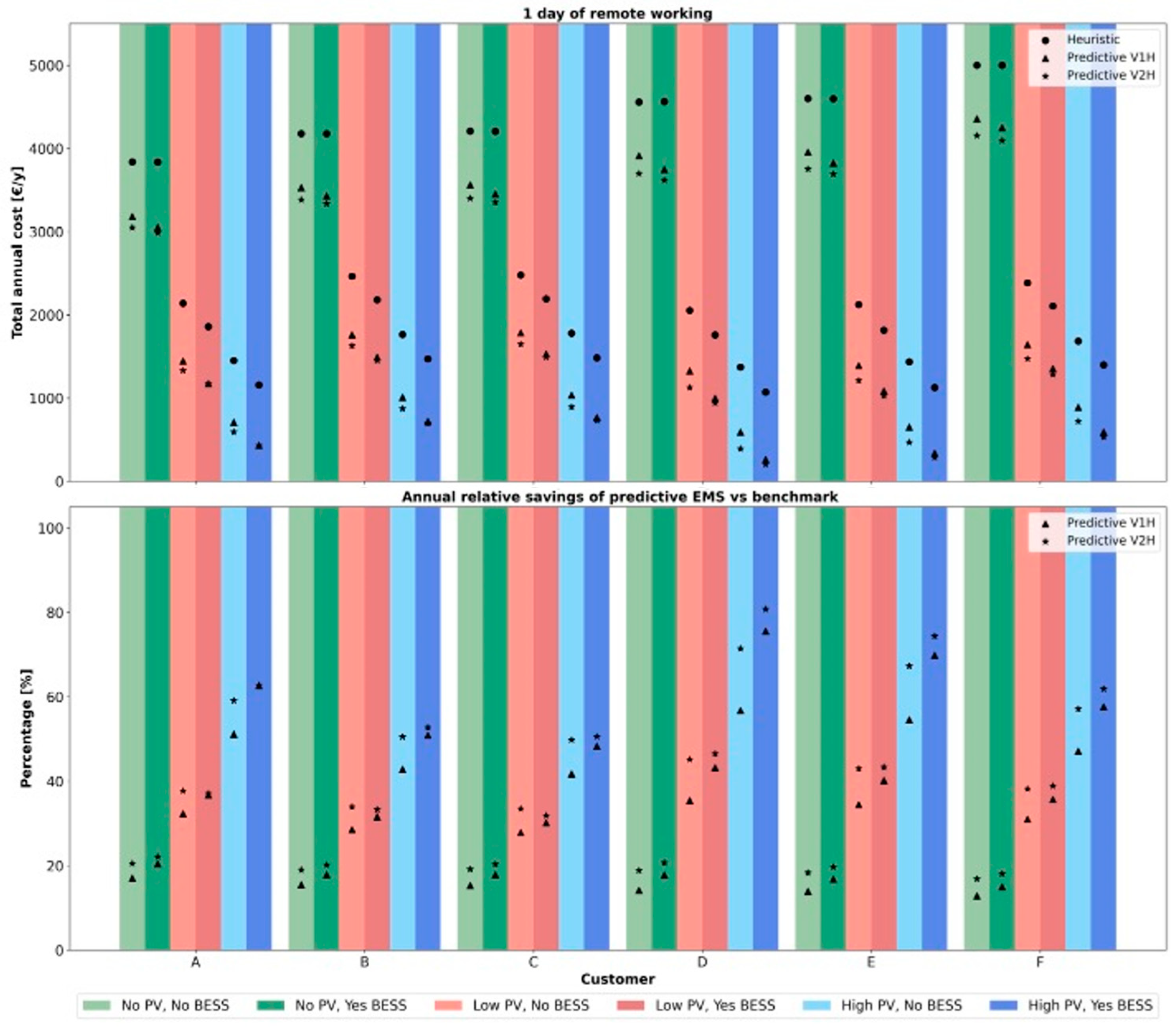
4.4. Case 2—1 Day of Remote Working

Remote working has a positive impact on household costs by reducing EV charging needs and enhancing flexibility. The V2H mode can effectively capitalize on this flexibility, leading to greater savings than those observed in Case 1, with close to 10% additional savings in configurations without BESS, as shown in Figure 13. Additionally, high PV penetration nearly eliminates costs over the analyzed period. Once again, in all these scenarios, the installation of BESS is not justified for any user. Comparing Figure 12 and Figure 14, it is possible to observe that PV self-consumption does not significantly vary between the two case studies. However, there is a slight improvement in configurations without BESS. The increased availability of the EV, thanks to the weekly remote working day, enables its charging through PV generation, as discussed in Section 4.1.

4.5. Case 3—2 Days of Remote Working

The conclusions drawn from earlier cases are equally applicable to this scenario. Specifically, configurations with high PV penetration generate revenues over the analyzed period due to the reduced additional demand from electric mobility, and V2H provides additional savings that are pushed to around 15% in configurations without BESS.

This case study aims to evaluate the implications of replacing the Nissan Leaf with a Tesla Model S, which boasts a larger capacity but higher on-road specific consumption, as detailed in Table 3. Examining total costs and relative savings presented in Table A5 and Table A6 reveals that the impact of higher on-road consumption outweighs the advantages of the greater capacity offered by the Tesla. This is notably apparent in users D and E with high PV penetration, where the Nissan Leaf results in revenues over the analyzed period, while switching to the Tesla Model S incurs costs. Nevertheless, the transition between EV models underscores the reliability of the developed methodology, demonstrating savings of up to 80% in V2H mode.

Regarding Case 4, the trends identified in earlier cases persist and are more pronounced. Once again, the installation of a BESS is not justified.

4.6. Ideal Performance Assessment

The scenario involving 2 days of remote working per week has been chosen to assess the home EMS performance under ideal conditions. This ideal case corresponds to an omniscient predictive EMS with null forecast errors. In this setting, the first layer timestep is reduced from 1 h to 15 min, and its forecasts perfectly align with PV and load measurements over a 24 h horizon. Consequently, in this case, the second layer operates with zero net demand forecast error, and the first-layer solution remains optimal. This analysis is crucial for assessing the influence of forecast errors related to PV and residential consumption on the system’s economic performance and quantifying the potential benefits of enhancing forecast accuracy. The comparison between the ideal and real home EMS has been conducted, focusing on both the management of household components and economic performance.

The operations shown in Figure 15 showcase the management of household components for the same days presented in Section 4.1 involving the same user and configuration. Notably, the ideal home EMS maximizes the utilization of previously outlined features, enabling the EV charging during hours with low electricity prices or aligning it with PV generation on remote working days. Furthermore, since no net demand forecast error is incurred, residential consumption peaks can be entirely satisfied using the EV or the BESS without the need to purchase electricity. Even with the ideal home EMS, the BESS is not considered during remote working days.

To quantify the disparity between the ideal and real home EMS total costs, performance indicators have been assessed in terms of absolute value of perfect forecast (AVPF) and relative value of perfect forecast (RVPF). The latter has been normalized by the total operating cost of the benchmark algorithm, as discussed in the relative savings presented in Section 3.1.2. This normalization allows the RVPF to represent the additional savings that would be achieved through a perfect forecast instead of a real one.

$${AVPF}_{EMS}\left[{\displaystyle \frac{€}{y}}\right]={TC}_{EMS}-{TC}_{EMS}^{id}$$

(16)

$${RVPF}_{EMS}[\%]={\displaystyle \frac{{TC}_{EMS}-{TC}_{EMS}^{id}}{\left|{TC}_{bench}\right|}}$$

(17)

These indicators are summarized in

Table 5. Absolute and relative value of perfect forecast of the home EMS in V1H and V2H modes.

User	PV	BESS	${\mathit{A}\mathit{V}\mathit{P}\mathit{F}}_{\mathit{V}1\mathit{H}}$	${\mathit{R}\mathit{V}\mathit{P}\mathit{F}}_{\mathit{V}1\mathit{H}}$	${\mathit{A}\mathit{V}\mathit{P}\mathit{F}}_{\mathit{V}2\mathit{H}}$	${\mathit{R}\mathit{V}\mathit{P}\mathit{F}}_{\mathit{V}2\mathit{H}}$
A	No	No	0.8	0.0%	22.4	0.7%
		Yes	22.0	0.6%	27.1	0.8%
	Low	No	16.2	1.0%	45.5	2.7%
		Yes	47.5	3.3%	60.3	4.3%
	High	No	16.7	1.7%	49.8	4.9%
		Yes	54.2	7.4%	67.9	9.2%
B	No	No	1.7	0.0%	57.9	1.5%
		Yes	59.7	1.6%	80.0	2.1%
	Low	No	6.0	0.3%	72.3	3.6%
		Yes	61.1	3.5%	104.2	6.0%
	High	No	4.5	0.3%	75.6	5.6%
		Yes	55.1	5.2%	100.7	9.6%
C	No	No	3.9	0.1%	61.6	1.6%
		Yes	50.0	1.3%	76.7	2.0%
	Low	No	12.6	0.6%	80.2	3.9%
		Yes	67.0	3.8%	107.5	6.1%
	High	No	10.7	0.8%	86.7	6.4%
		Yes	66.1	6.2%	115.1	10.7%
D	No	No	0.8	0.0%	22.1	0.5%
		Yes	19.9	0.5%	27.8	0.7%
	Low	No	14.1	0.9%	51.1	3.2%
		Yes	50.9	3.8%	68.2	5.1%
	High	No	15.2	1.6%	55.4	5.9%
		Yes	54.0	8.2%	74.7	11.4%
E	No	No	2.1	0.1%	66.0	1.6%
		Yes	67.7	1.6%	87.6	2.1%
	Low	No	5.8	0.3%	92.1	5.4%
		Yes	78.5	5.6%	120.8	8.7%
	High	No	6.4	0.6%	95.8	9.5%
		Yes	81.1	11.5%	125.9	17.8%
F	No	No	2.8	0.1%	83.8	1.8%
		Yes	78.7	1.7%	112.6	2.5%
	Low	No	11.2	0.6%	106.6	5.5%
		Yes	87.0	5.2%	140.0	8.3%
	High	No	9.5	0.8%	102.9	8.2%
		Yes	82.2	8.3%	136.3	13.8%

, and total costs are collected in

Table A9. Total annual operating cost of the benchmark algorithm and real and ideal EMS in V1H and V2H for the ideal performance assessment of Case 2.

User	PV	BESS	${\mathit{T}\mathit{C}}_{\mathit{b}\mathit{e}\mathit{n}\mathit{c}\mathit{h}}$	${\mathit{T}\mathit{C}}_{\mathit{V}1\mathit{H}}$	${\mathit{T}\mathit{C}}_{\mathit{V}1\mathit{H}}^{\mathit{i}\mathit{d}}$	${\mathit{T}\mathit{C}}_{\mathit{V}2\mathit{H}}$	${\mathit{T}\mathit{C}}_{\mathit{V}2\mathit{H}}^{\mathit{i}\mathit{d}}$
A	No	No	3397.8	2843.6	2842.8	2706.8	2684.4
		Yes	3397.4	2712.1	2690.1	2643.3	2616.2
	Low	No	1694.0	1044.4	1028.3	902.2	856.7
		Yes	1418.5	787.8	740.3	774.5	714.2
	High	No	1013.6	305.2	288.4	155.5	105.7
		Yes	735.5	40.4	−13.9	28.6	−39.4
B	No	No	3742.4	3192.6	3190.9	3047.5	2989.6
		Yes	3741.2	3095.8	3036.1	2995.9	2915.9
	Low	No	2026.9	1356.0	1350.0	1185.4	1113.0
		Yes	1750.7	1103.4	1042.4	1056.0	951.8
	High	No	1337.9	602.4	597.9	419.6	344.1
		Yes	1053.1	326.7	271.6	281.9	181.2
C	No	No	3768.1	3224.2	3220.3	3064.7	3003.1
		Yes	3769.2	3118.7	3068.8	3011.4	2934.7
	Low	No	2038.2	1389.0	1376.4	1219.6	1139.5
		Yes	1768.5	1154.5	1087.5	1097.7	990.2
	High	No	1348.8	635.5	624.8	451.9	365.2
		Yes	1073.8	382.6	316.5	325.3	210.2
D	No	No	4125.3	3575.4	3574.6	3353.6	3331.5
		Yes	4124.5	3411.2	3391.2	3273.8	3246.0
	Low	No	1616.6	923.4	909.3	675.4	624.3
		Yes	1337.0	606.2	555.3	527.0	458.9
	High	No	937.4	192.3	177.1	−63.9	−119.2
		Yes	655.2	−133.6	−187.6	−211.9	−286.7
E	No	No	4165.1	3619.2	3617.1	3422.7	3356.7
		Yes	4164.4	3492.1	3424.4	3358.4	3270.8
	Low	No	1693.5	986.2	980.4	757.3	665.2
		Yes	1395.0	693.3	614.8	613.4	492.6
	High	No	1009.2	247.3	241.0	9.0	−86.7
		Yes	706.5	−51.6	−132.6	−133.4	−259.4
F	No	No	4562.4	4019.1	4016.3	3809.0	3725.2
		Yes	4563.5	3913.6	3834.9	3747.3	3634.7
	Low	No	1949.8	1245.6	1234.4	1029.5	922.9
		Yes	1688.8	972.3	885.3	880.0	740.0
	High	No	1254.6	493.6	484.1	268.2	165.3
		Yes	989.0	208.4	126.2	117.7	−18.6

of Appendix B.

As expected, AVPF is more pronounced in configurations where increasing degrees of freedom can be leveraged, such as those involving BESS and the ideal home EMS in V2H mode. A noteworthy observation from this analysis is that regardless of the forecast performance quality, the additional performance between real and ideal home EMS in absolute terms would be at most around 140 €/year and would not provide more than 10% of additional savings with respect to the heuristic benchmark for most configurations. This means that (i) enhancing the accuracy of PV and residential consumption forecasters may not yield a noticeable improvement in performance, and (ii) the proposed EMS is effective in balancing forecast errors with limited economic penalties.

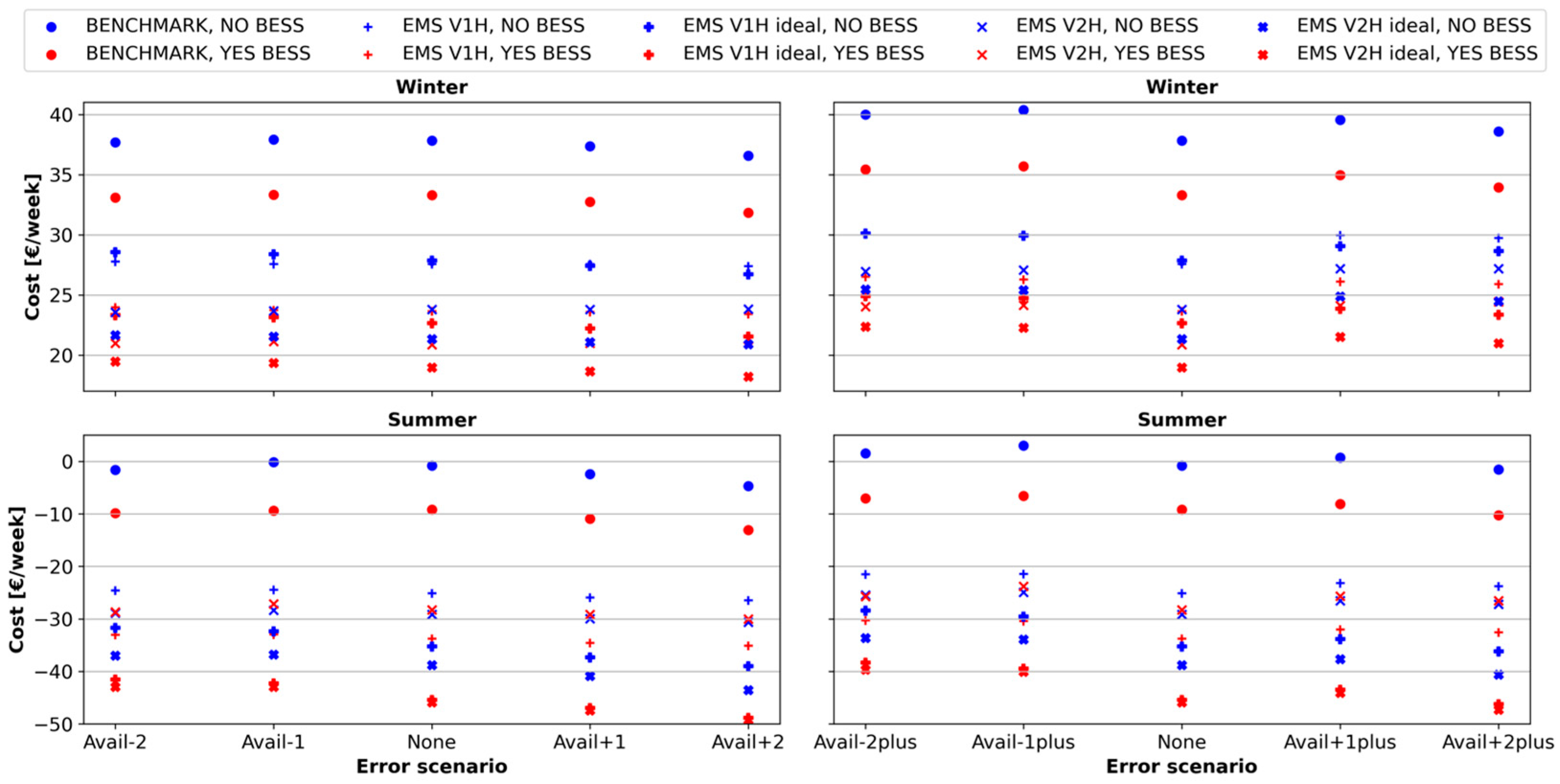
4.7. Impact of EV Usage Forecast Errors

Another critical aspect to consider is the impact of different types of errors in forecasting EV availability and usage throughout the day. This assessment was conducted by simulating various scenarios with systematic errors in the forecast of the EV use in terms of time periods and/or energy consumed in the trop. The home EMS responds to these forecast errors by updating the EV use forecast with the measurement and re-executing the first layer to adjust the optimal setpoints followed by the second layer. The tests were made for the case with user E (with 2 days of remote working,) with a 6 kW PV plant (large) considering a winter and a summer week. Different scenarios are considered, with V1H and V2H modes and with and without the BESS.

Two types of errors in EV use forecasts were evaluated: forecast errors in terms of time periods at home and forecast errors in distance traveled during the trip (i.e., energy consumed). Availability forecast errors of +1 h, (meaning that the EV leaves the house and then returns to the house 1 h after the forecasted value), −1 h, +2 h, and −2 h were considered. These errors were labeled as Avail+1, Avail−1, Avail+2, and Avail−2. Distance (energy consumption) forecast errors were considered alongside availability errors by adding unexpected trips of 20 km during lunchtime on Sunday and 10 km in the morning of one of the remote working days. The test cases with both availability forecast errors and distance forecast errors are labeled as “Avail+1 plus”, “Avail−1 plus”, etc.

The ideal home EMS, as defined in Section 4.6, was employed to assess the impact of EV forecast errors and served as the reference for the relative difference (RD) performance indicator, computed as follows:

$$RD [\%]={\displaystyle \frac{{TC}_{EMS}^{Real}-{TC}_{EMS}^{ideal}}{{TC}_{EMS}^{ideal}}}$$

(18)

The results of the tests are available in

Table A10. Total weekly operating costs of the tested EMS during a winter and summer week of user E, equipped with a 6 kW PV field, for different EV forecast error scenarios.

Season	Configuration		None	Avail−2	Avail−1	Avail+1	Avail+2	Avail−2 Plus	Avail−1 Plus	Avail+1 Plus	Avail+2 Plus
Winter	NO BESS	${\mathit{T}\mathit{C}}_{\mathit{b}\mathit{e}\mathit{n}\mathit{c}\mathit{h}}$	37.82	37.68	37.92	37.37	36.57	40.00	40.37	39.56	38.60
		${\mathit{T}\mathit{C}}_{\mathit{V}1\mathit{H}}^{\mathit{r}\mathit{e}\mathit{a}\mathit{l}}$	27.56	27.76	27.57	27.57	27.39	30.16	29.97	29.96	29.74
		${\mathit{T}\mathit{C}}_{\mathit{V}1\mathit{H}}^{\mathit{i}\mathit{d}\mathit{e}\mathit{a}\mathit{l}}$	27.85	28.55	28.37	27.41	26.71	30.10	29.93	29.05	28.66
		${\mathit{T}\mathit{C}}_{\mathit{V}2\mathit{H}}^{\mathit{r}\mathit{e}\mathit{a}\mathit{l}}$	23.80	23.55	23.68	23.80	23.82	26.94	27.05	27.19	27.18
		${\mathit{T}\mathit{C}}_{\mathit{V}2\mathit{H}}^{\mathit{i}\mathit{d}\mathit{e}\mathit{a}\mathit{l}}$	21.33	21.64	21.54	21.08	20.90	25.46	25.41	24.88	24.47
		${\mathit{R}\mathit{D}}_{\mathit{V}1\mathit{H}}$	−1%	−3%	−3%	1%	3%	0%	0%	3%	4%
		${\mathit{R}\mathit{D}}_{\mathit{V}2\mathit{H}}$	12%	9%	10%	13%	14%	6%	6%	9%	11%
	YES BESS	${\mathit{T}\mathit{C}}_{\mathit{b}\mathit{e}\mathit{n}\mathit{c}\mathit{h}}$	33.30	33.09	33.34	32.74	31.84	35.44	35.69	34.97	33.94
		${\mathit{T}\mathit{C}}_{\mathit{V}1\mathit{H}}^{\mathit{r}\mathit{e}\mathit{a}\mathit{l}}$	23.65	23.98	23.73	23.60	23.43	26.51	26.26	26.11	25.88
		${\mathit{T}\mathit{C}}_{\mathit{V}1\mathit{H}}^{\mathit{i}\mathit{d}\mathit{e}\mathit{a}\mathit{l}}$	22.65	23.32	23.15	22.21	21.54	24.90	24.73	23.85	23.36
		${\mathit{T}\mathit{C}}_{\mathit{V}2\mathit{H}}^{\mathit{r}\mathit{e}\mathit{a}\mathit{l}}$	20.87	20.98	21.12	20.98	21.30	24.01	24.16	24.13	24.44
		${\mathit{T}\mathit{C}}_{\mathit{V}2\mathit{H}}^{\mathit{i}\mathit{d}\mathit{e}\mathit{a}\mathit{l}}$	18.96	19.46	19.36	18.64	18.20	22.36	22.26	21.52	21.00
		${\mathit{R}\mathit{D}}_{\mathit{V}1\mathit{H}}$	4%	3%	3%	6%	9%	6%	6%	9%	11%
		${\mathit{R}\mathit{D}}_{\mathit{V}2\mathit{H}}$	10%	8%	9%	13%	17%	7%	9%	12%	16%
Summer	NO BESS	${\mathit{T}\mathit{C}}_{\mathit{b}\mathit{e}\mathit{n}\mathit{c}\mathit{h}}$	−0.83	−1.60	−0.12	−2.41	−4.68	1.56	3.04	0.75	−1.52
		${\mathit{T}\mathit{C}}_{\mathit{V}1\mathit{H}}^{\mathit{r}\mathit{e}\mathit{a}\mathit{l}}$	−25.13	−24.58	−24.43	−25.96	−26.49	−21.53	−21.47	−23.17	−23.81
		${\mathit{T}\mathit{C}}_{\mathit{V}1\mathit{H}}^{\mathit{i}\mathit{d}\mathit{e}\mathit{a}\mathit{l}}$	−35.27	−31.69	−32.34	−37.31	−38.98	−28.42	−29.58	−33.81	−36.18
		${\mathit{T}\mathit{C}}_{\mathit{V}2\mathit{H}}^{\mathit{r}\mathit{e}\mathit{a}\mathit{l}}$	−29.12	−28.87	−28.35	−29.94	−30.59	−25.45	−24.94	−26.52	−27.17
		${\mathit{T}\mathit{C}}_{\mathit{V}2\mathit{H}}^{\mathit{i}\mathit{d}\mathit{e}\mathit{a}\mathit{l}}$	−38.81	−36.96	−36.78	−40.85	−43.54	−33.61	−33.92	−37.67	−40.58
		${\mathit{R}\mathit{D}}_{\mathit{V}1\mathit{H}}$	29%	22%	24%	30%	32%	24%	27%	31%	34%
		${\mathit{R}\mathit{D}}_{\mathit{V}2\mathit{H}}$	25%	22%	23%	27%	30%	24%	26%	30%	33%
	YES BESS	${\mathit{T}\mathit{C}}_{\mathit{b}\mathit{e}\mathit{n}\mathit{c}\mathit{h}}$	−9.18	−9.83	−9.38	−10.90	−13.04	−7.04	−6.59	−8.12	−10.25
		${\mathit{T}\mathit{C}}_{\mathit{V}1\mathit{H}}^{\mathit{r}\mathit{e}\mathit{a}\mathit{l}}$	−33.75	−33.01	−32.96	−34.57	−35.12	−30.28	−30.41	−32.04	−32.59
		${\mathit{T}\mathit{C}}_{\mathit{V}1\mathit{H}}^{\mathit{i}\mathit{d}\mathit{e}\mathit{a}\mathit{l}}$	−45.44	−41.57	−42.28	−46.95	−48.85	−38.33	−39.48	−43.50	−46.26
		${\mathit{T}\mathit{C}}_{\mathit{V}2\mathit{H}}^{\mathit{r}\mathit{e}\mathit{a}\mathit{l}}$	−28.30	−28.65	−27.12	−29.15	−30.05	−25.73	−23.77	−25.69	−26.56
		${\mathit{T}\mathit{C}}_{\mathit{V}2\mathit{H}}^{\mathit{i}\mathit{d}\mathit{e}\mathit{a}\mathit{l}}$	−45.89	−42.95	−42.97	−47.41	−50.14	−39.69	−40.06	−44.07	−47.33
		${\mathit{R}\mathit{D}}_{\mathit{V}1\mathit{H}}$	26%	21%	22%	26%	28%	21%	23%	26%	30%
		${\mathit{R}\mathit{D}}_{\mathit{V}2\mathit{H}}$	38%	33%	37%	39%	40%	35%	41%	42%	44%

and Figure 16. Figure 16 illustrates total weekly costs achieved by the benchmark algorithm and the EMS (real and ideal EMS without forecast errors).

As shown in Table A10 and in Figure 16, the real home EMS consistently outperforms the benchmark algorithm (dots), with significantly lower operational costs across all considered EV error scenarios and configurations. The weekly costs remain relatively consistent across the error scenarios once the home EMS mode and configuration are selected. However, in the winter week, the relative difference between real and ideal EMS consistently stays below 20%, while in the summer week, it consistently exceeds 20%, reaching over 40% in certain scenarios. This discrepancy is attributed to higher PV generation in the summer, where an error in the EV forecast leads to reduced local utilization of the abundant renewable generation. Therefore, improving the accuracy of EV usage forecasts can significantly enhance the consistency of home EMS performances.

5. Conclusions and Further Developments

This paper presents a hierarchical EMS designed for the economic dispatch and control of a grid-connected smart home. The first layer of the proposed algorithm addresses the strategic planning problem over the next 24 h, employing a mixed-integer linear program (MILP) formulation to define optimal power setpoints for the dispatchable components, the stationary battery and the electric vehicle. The second layer refines the first layer’s power setpoints using a heuristic rule-based algorithm to balance net demand forecast errors associated with residential consumption and photovoltaic generation. A rolling horizon approach updates the first layer solution every 1 h.

The performance of the home EMS is evaluated against a non-predictive heuristic benchmark algorithm, reflecting the management commonly found in current smart homes. The assessment covers various case studies, incorporating different users, photovoltaic generation penetration, BESS presence, monodirectional or bidirectional EV charging, EV models, and EV weekly commutes. The home EMS proves to be cost-effective, demonstrating yearly cost savings above 20% in all cases and up to 900 €/y in configurations with large PV plants. The economic advantage of the EMS with respect to the benchmark heuristic algorithm remains high also in the case of systematic forecast errors in the use of the EV.

The findings also indicate that under the current Italian residential electricity pricing scheme, installing a stationary BESS is not economically advantageous. However, integrating a smart home within a broader energy ecosystem—such as a renewable energy community—could significantly alter the financial dynamics. In such contexts, alternative pricing schemes and compensation mechanisms for services provided by the BESS (e.g., energy arbitrage, grid support) could enhance economic viability, representing an interesting direction for future research.

Bidirectional chargers can provide additional savings, which increase with the number of weekly remote working days, reaching around 10–15% in configurations without BESS.

The results indicate that the economic gain of the EMS compared to the benchmark heuristic algorithm can be even higher if the accuracy of the forecasts is improved. In this regard, the preliminary tests have shown that improvement of the forecast of the use of the EV has a larger effect, especially in the summer, for plants with large PV plant (leading 40% potential increased revenues) than the forecast of PV and domestic loads (leading to a potential further revenues or cost saving of 10%).

Future developments of the EMS will focus on implementing stochastic methodologies able to mitigate the effect of the EV use forecast accuracy on the solution optimality.

References

1. European Commission EU Solar Energy Strategy. Available online: https://eur-lex.europa.eu/legal-content/EN/TXT/?uri=COM%3A2022%3A221%3AFIN&qid=1653034500503 (accessed on 25 September 2023).
2. SolarPower Europe Annual Rooftop and Utility Scale Installations in the EU. Available online: https://www.solarpowereurope.org/advocacy/solar-saves/fact-figures/annual-rooftop-and-utility-scale-installations-in-the-eu (accessed on 21 November 2023).
3. European Automobile Manufacturers’ Association ACEA EU New Car Registrations June 2023. Available online: https://www.acea.auto/pc-registrations/new-car-registrations-17-8-in-june-battery-electric-15-1-market-share/ (accessed on 25 September 2023).
4. European Commission Smart Grids and Meters. Available online: https://energy.ec.europa.eu/topics/markets-and-consumers/smart-grids-and-meters_en (accessed on 14 November 2023).
5. European Commission EU Strategy on Energy System Integration. Available online: https://energy.ec.europa.eu/topics/energy-systems-integration/eu-strategy-energy-system-integration_en (accessed on 14 November 2023).
6. Ministero dell’Ambiente e della Sicurezza Energetica. Piano Nazionale Integrato per l’Energia e per Il Clima—2023; Ministero dell’Ambiente e della Sicurezza: Rome, Italy, 2023. [Google Scholar]
7. Ministero dello Sviluppo Economico; Ministero dell’Ambiente e della Tutela del Territorio e del Mare; Ministero delle Infrastrutture e dei Trasporti. Piano Nazionale Integrato per l’Energia e per Il Clima; Rome, Italy. 2019. Available online: https://energy.ec.europa.eu/system/files/2020-01/it_final_necp_main_it_0.pdf (accessed on 16 February 2025).
8. Beaudin, M.; Zareipour, H. Home Energy Management Systems: A Review of Modelling and Complexity. Renew. Sustain. Energy Rev. 2015, 45, 318–335. [Google Scholar] [CrossRef]
9. Battula, A.R.; Vuddanti, S.; Salkuti, S.R. Review of Energy Management System Approaches in Microgrids. Energies 2021, 14, 5459. [Google Scholar] [CrossRef]
10. Wu, X.; Hu, X.; Yin, X.; Moura, S.J. Stochastic Optimal Energy Management of Smart Home with PEV Energy Storage. IEEE Trans. Smart Grid 2018, 9, 2065–2075. [Google Scholar] [CrossRef]
11. Wu, X.; Hu, X.; Moura, S.; Yin, X.; Pickert, V. Stochastic Control of Smart Home Energy Management with Plug-in Electric Vehicle Battery Energy Storage and Photovoltaic Array. J. Power Sources 2016, 333, 203–212. [Google Scholar] [CrossRef]
12. Shin, M.; Choi, D.-H.; Kim, J. Cooperative Management for PV/ESS-Enabled Electric Vehicle Charging Stations: A Multiagent Deep Reinforcement Learning Approach. IEEE Trans. Ind. Inform. 2020, 16, 3493–3503. [Google Scholar] [CrossRef]
13. Wi, Y.-M.; Lee, J.-U.; Joo, S.-K. Electric Vehicle Charging Method for Smart Homes/Buildings with a Photovoltaic System. IEEE Trans. Consum. Electron. 2013, 59, 323–328. [Google Scholar] [CrossRef]
14. Erdinc, O. Economic Impacts of Small-Scale Own Generating and Storage Units, and Electric Vehicles under Different Demand Response Strategies for Smart Households. Appl. Energy 2014, 126, 142–150. [Google Scholar] [CrossRef]
15. Paterakis, N.G.; Erdinç, O.; Bakirtzis, A.G.; Catalão, J.P.S. Optimal Household Appliances Scheduling Under Day-Ahead Pricing and Load-Shaping Demand Response Strategies. IEEE Trans. Ind. Inf. 2015, 11, 1509–1519. [Google Scholar] [CrossRef]
16. Tostado-Véliz, M.; León-Japa, R.S.; Jurado, F. Optimal Electrification of Off-Grid Smart Homes Considering Flexible Demand and Vehicle-to-Home Capabilities. Appl. Energy 2021, 298, 117184. [Google Scholar] [CrossRef]
17. Paterakis, N.G.; Pappi, I.N.; Catalão, J.P.S.; Erdinc, O. Optimal Operation of Smart Houses by a Real-Time Rolling Horizon Algorithm. In Proceedings of the 2016 IEEE Power and Energy Society General Meeting (PESGM), Boston, MA, USA, 16 July 2016; pp. 1–5. [Google Scholar]
18. Erdinc, O.; Paterakis, N.G.; Pappi, I.N.; Bakirtzis, A.G.; Catalão, J.P.S. A New Perspective for Sizing of Distributed Generation and Energy Storage for Smart Households under Demand Response. Appl. Energy 2015, 143, 26–37. [Google Scholar] [CrossRef]
19. Pilotti, L.; Moretti, L.; Martelli, E.; Manzolini, G. Optimal E-Fleet Charging Station Design with V2G Capability. Sustain. Energy Grids Netw. 2023, 36, 101220. [Google Scholar] [CrossRef]
20. Tostado-Véliz, M.; Gurung, S.; Jurado, F. Efficient Solution of Many-Objective Home Energy Management Systems. Int. J. Electr. Power Energy Syst. 2022, 136, 107666. [Google Scholar] [CrossRef]
21. Tostado-Véliz, M.; Hasanien, H.M.; Kamel, S.; Turky, R.A.; Jurado, F.; Elkadeem, M.R. Multiobjective Home Energy Management Systems in Nearly-Zero Energy Buildings under Uncertainties Considering Vehicle-to-Home: A Novel Lexicographic-Based Stochastic-Information Gap Decision Theory Approach. Electr. Power Syst. Res. 2023, 214, 108946. [Google Scholar] [CrossRef]
22. Zhang, D.; Evangelisti, S.; Lettieri, P.; Papageorgiou, L.G. Economic and Environmental Scheduling of Smart Homes with Microgrid: DER Operation and Electrical Tasks. Energy Convers. Manag. 2016, 110, 113–124. [Google Scholar] [CrossRef]
23. Erdinç, F.G. Rolling Horizon Optimization Based Real-Time Energy Management of a Residential Neighborhood Considering PV and ESS Usage Fairness. Appl. Energy 2023, 344, 121275. [Google Scholar] [CrossRef]
24. Thomas, D.; Deblecker, O.; Ioakimidis, C.S. Optimal Operation of an Energy Management System for a Grid-Connected Smart Building Considering Photovoltaics’ Uncertainty and Stochastic Electric Vehicles’ Driving Schedule. Appl. Energy 2018, 210, 1188–1206. [Google Scholar] [CrossRef]
25. Meng, L.; Sanseverino, E.R.; Luna, A.; Dragicevic, T.; Vasquez, J.C.; Guerrero, J.M. Microgrid Supervisory Controllers and Energy Management Systems: A Literature Review. Renew. Sustain. Energy Rev. 2016, 60, 1263–1273. [Google Scholar] [CrossRef]
26. Moretti, L.; Polimeni, S.; Meraldi, L.; Raboni, P.; Leva, S.; Manzolini, G. Assessing the Impact of a Two-Layer Predictive Dispatch Algorithm on Design and Operation of off-Grid Hybrid Microgrids. Renew. Energy 2019, 143, 1439–1453. [Google Scholar] [CrossRef]
27. Esmaeel Nezhad, A.; Rahimnejad, A.; Nardelli, P.H.J.; Gadsden, S.A.; Sahoo, S.; Ghanavati, F. A Shrinking Horizon Model Predictive Controller for Daily Scheduling of Home Energy Management Systems. IEEE Access 2022, 10, 29716–29730. [Google Scholar] [CrossRef]
28. Jiang, Q.; Xue, M.; Geng, G. Energy Management of Microgrid in Grid-Connected and Stand-Alone Modes. IEEE Trans. Power Syst. 2013, 28, 3380–3389. [Google Scholar] [CrossRef]
29. Fusco, A.; Gioffré, D.; Leva, S.; Manzolini, G.; Martelli, E.; Moretti, L. Predictive Energy Management System for a PV-BESS System Bidding on Day-Ahead and Intra-Day Electricity Markets. In Proceedings of the 2023 IEEE Belgrade PowerTech, Belgrade, Serbia, 25–29 June 2023; pp. 1–6. [Google Scholar]
30. Shapiro, A. On Complexity of Multistage Stochastic Programs. Oper. Res. Lett. 2006, 34, 1–8. [Google Scholar] [CrossRef]
31. Kim, M.; Park, T.; Jeong, J.; Kim, H. Stochastic Optimization of Home Energy Management System Using Clustered Quantile Scenario Reduction. Appl. Energy 2023, 349, 121555. [Google Scholar] [CrossRef]
32. Castelli, A.F.; Moretti, L.; Manzolini, G.; Martelli, E. Robust Optimization of Seasonal, Day-Ahead and Real Time Operation of Aggregated Energy Systems. Int. J. Electr. Power Energy Syst. 2023, 152, 109190. [Google Scholar] [CrossRef]
33. Moretti, L.; Martelli, E.; Manzolini, G. An Efficient Robust Optimization Model for the Unit Commitment and Dispatch of Multi-Energy Systems and Microgrids. Appl. Energy 2020, 261, 113859. [Google Scholar] [CrossRef]
34. Gestore Servizi Energetici (GSE). Ritiro Dedicato; GSE: Roma, Italy, 2023; Available online: https://www.gse.it/servizi-per-te/fotovoltaico/ritiro-dedicato (accessed on 12 October 2023).
35. Gestore Mercati Energetici (GME). Vademecum Della Borsa Elettrica; GME: Roma, Italy, 2009. [Google Scholar]
36. Imani, M.H.; Bompard, E.; Colella, P.; Huang, T. Forecasting Electricity Price in Different Time Horizons: An Application to the Italian Electricity Market. IEEE Trans. Ind. Appl. 2021, 57, 5726–5736. [Google Scholar] [CrossRef]
37. Gestore Mercati Energetici (GME). Statistiche; GME: Roma, Italy, 2023; Available online: https://www.mercatoelettrico.org/It/download/DatiStorici.aspx (accessed on 23 October 2023).
38. Melhem, F.Y.; Grunder, O.; Hammoudan, Z.; Moubayed, N. Energy Management in Electrical Smart Grid Environment Using Robust Optimization Algorithm. IEEE Trans. Ind. Appl. 2018, 54, 2714–2726. [Google Scholar] [CrossRef]
39. Boynuegri, A.R.; Yagcitekin, B.; Baysal, M.; Karakas, A.; Uzunoglu, M. Energy Management Algorithm for Smart Home with Renewable Energy Sources. In Proceedings of the International Conference on Power Engineering, Energy and Electrical Drives, Istanbul, Turkey, 13–17 December 2013; pp. 1753–1758. [Google Scholar]
40. Bynum, M.L.; Hackebeil, G.A.; Hart, W.E.; Laird, C.D.; Nicholson, B.L.; Siirola, J.D.; Watson, J.-P.; Woodruff, D.L. Pyomo—Optimization Modeling in Python, 3rd ed.; Springer Science & Business Media: Berlin/Heidelberg, Germany, 2021; Volume 67. [Google Scholar]
41. Hart, W.; Watson, J.-P.; Woodruff, D.; Watson, J.-P. Pyomo: Modeling and Solving Mathematical Programs in Python. Math. Program. Comput. 2011, 3, 219–260. [Google Scholar] [CrossRef]
42. The Leader in Decision Intelligence Technology-Gurobi Optimization. Gurobi Optimizer Reference Manual; The Leader in Decision Intelligence Technology-Gurobi Optimization: Beaverton, OR, USA, 2021. [Google Scholar]
43. Gestore dei Servizi Energetici (GSE). Rapporto Statistico—Solare Fotovoltaico 2022; GSE: Roma, Italy, 2023. [Google Scholar]
44. Niu, S.; Zhao, Q.; Chen, H.; Niu, S.; Jian, L. Noncooperative Metal Object Detection Using Pole-to-Pole EM Distribution Characteristics for Wireless EV Charger Employing DD Coils. IEEE Trans. Ind. Electron. 2024, 71, 6335–6344. [Google Scholar] [CrossRef]
Figure 1. Schematic representation of a smart home integrating an electric vehicle, battery storage, rooftop PV, and household appliances.
Energies 18 01774 g001
Figure 2. Structure of the EMS.
Energies 18 01774 g002
Figure 3. Boxplot of the day-ahead market clearing price from 28 January 2022 until 28 January 2023.
Energies 18 01774 g003
Figure 4. Second layer heuristic strategy block-flow scheme.
Energies 18 01774 g004
Figure 5. Block-flow diagram of the benchmark algorithm.
Energies 18 01774 g005
Figure 6. PV forecast WMAE and SMAPE.
Energies 18 01774 g006
Figure 7. Residential consumption forecast WMAE and SMAPE. Each colored line corresponds to a user name, following the nomenclature presented in Table 2.
Energies 18 01774 g007
Figure 8. Comparison between heuristic and predictive operations—power balance.
Energies 18 01774 g008
Figure 9. Comparison between heuristic and predictive operations—EV management.
Energies 18 01774 g009
Figure 10. Comparison between heuristic and predictive operations—BESS management.
Energies 18 01774 g010
Figure 11. Case 1 economic performances.
Energies 18 01774 g011
Figure 12. Case 1 PV self-consumption.
Energies 18 01774 g012
Figure 13. Case 2 economic performances.
Energies 18 01774 g013
Figure 14. Case 2 PV self-consumption.
Energies 18 01774 g014
Figure 15. Home EMS ideal predictive operations.
Energies 18 01774 g015
Figure 16. Total weekly costs of benchmark algorithm and home EMS in V1H and V2H modes under various EV errors scenarios for winter and summer weeks.
Energies 18 01774 g016