
Impact of Climate Change on Wind Power Generation Studied Using Multivariate Copula Downscaling: A Case Study in Northwestern China

Abstract
1. Introduction
2. Methodology
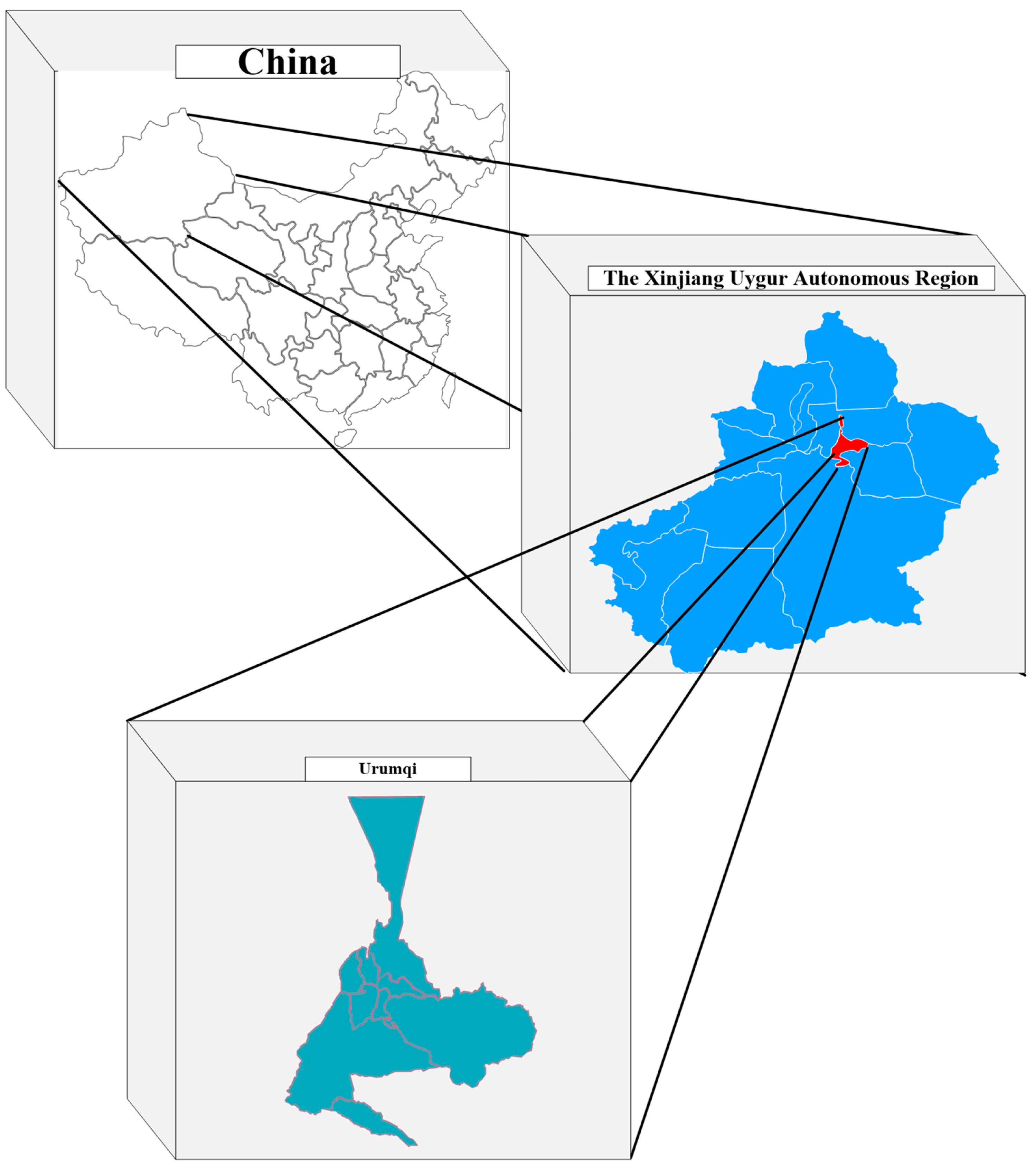
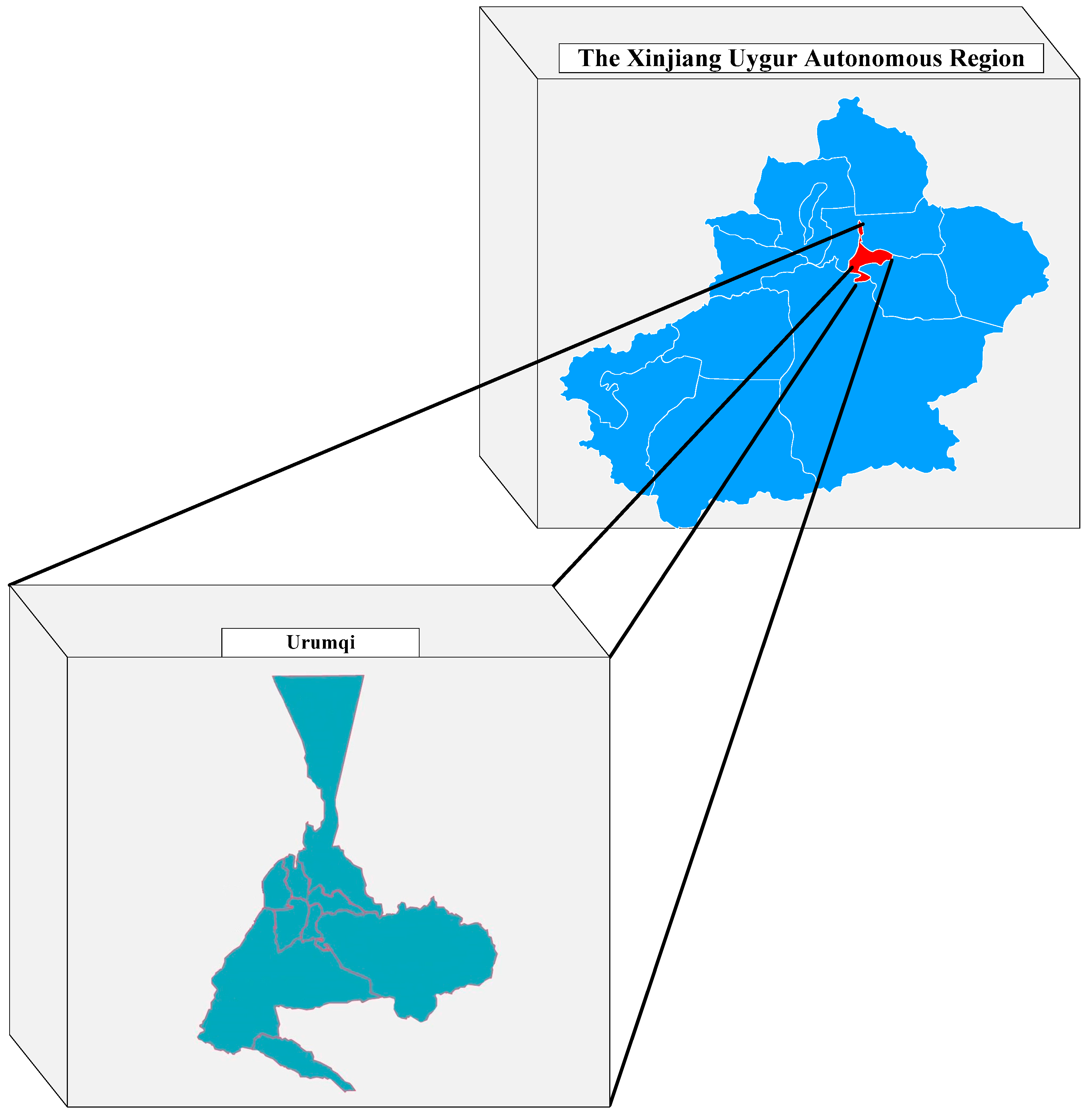
2.1. Study Site
2.2. Copula Method
2.3. Common Copula Functions
- (1)
- Gaussian Copula
- (2)
- t-Copula
- (3)
- Archimedean Copula
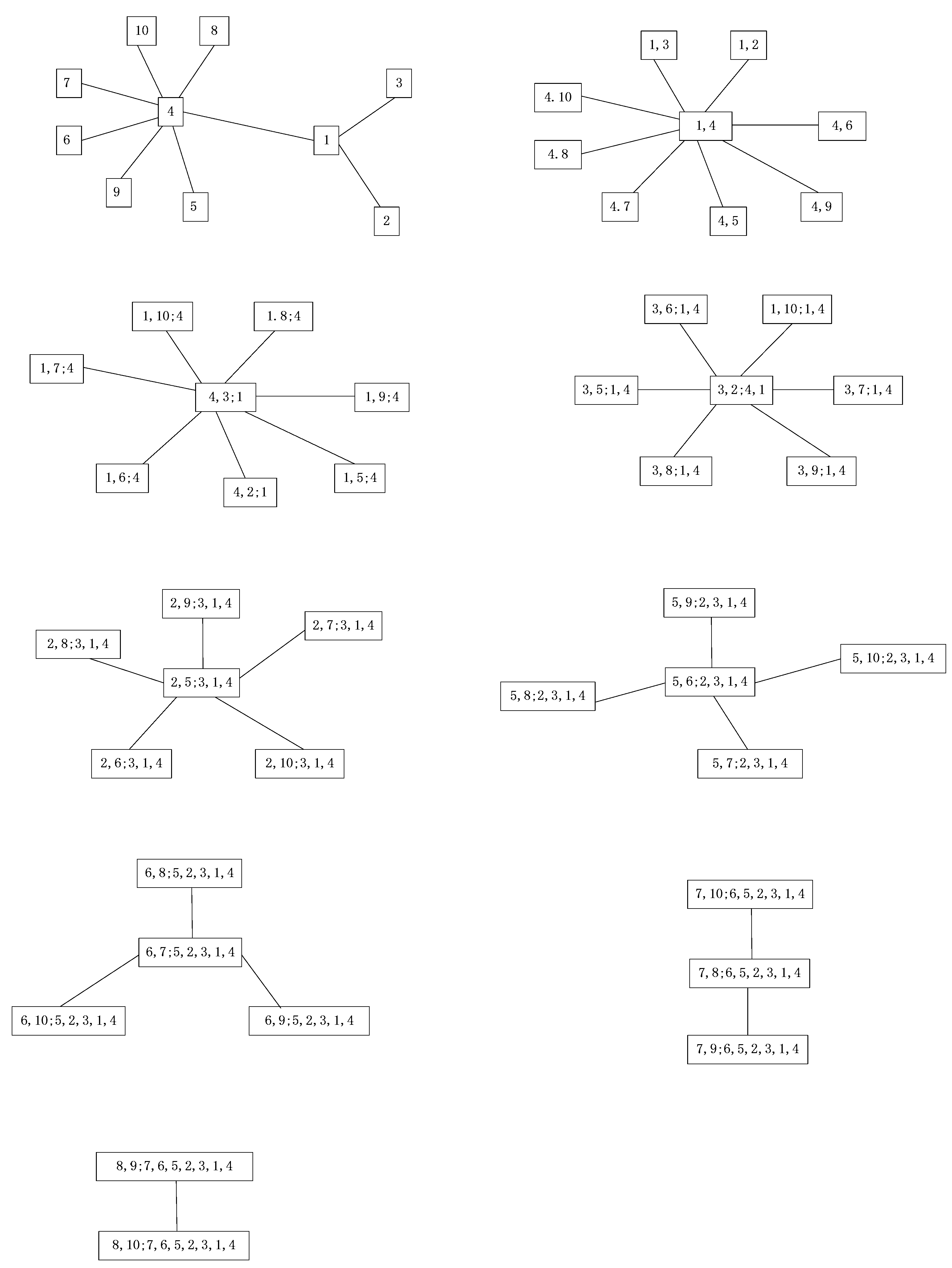
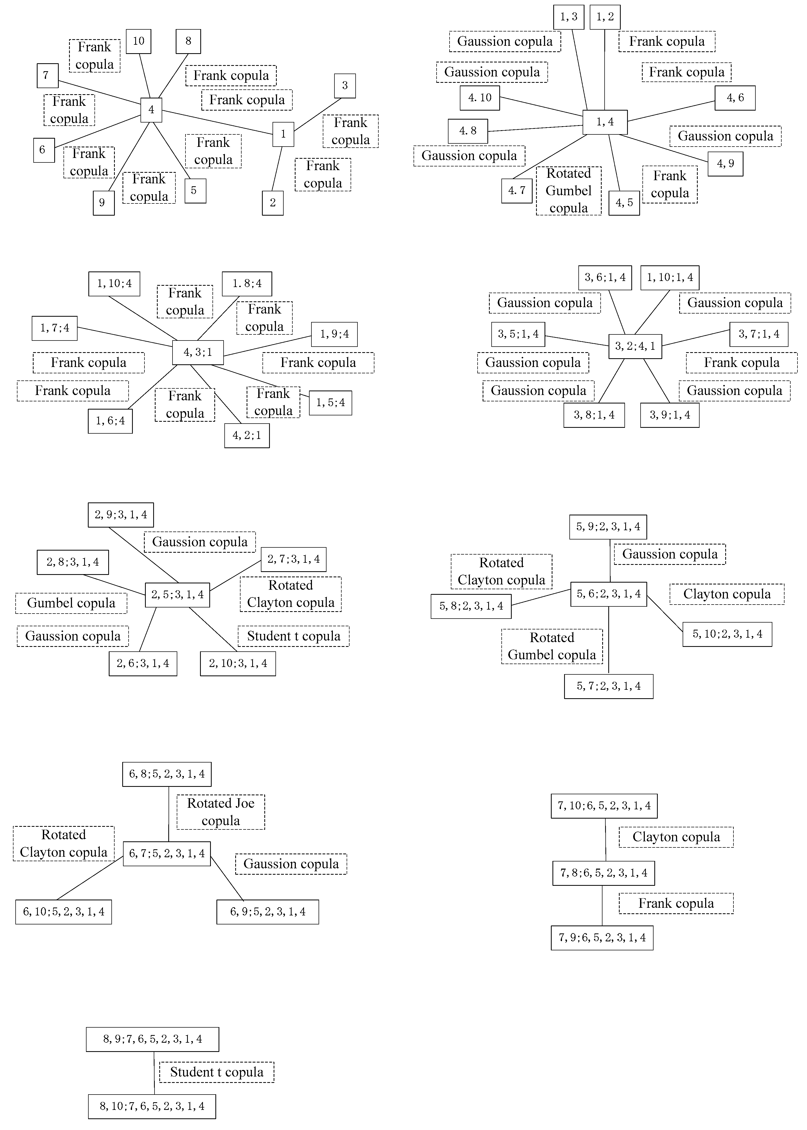
2.4. MvCD Based on Pair-Copula Method
- 1.
- The first layer pair-copula sequence was constructed by bivariate copula functions of one random variable with other random variables:
- 2.
- The second layer condition pair-copula sequence is constructed by distribution functions of (1) as new random variable sequences:
- 3.
- Repeating step (2) until the last one bivariate copula reveals
2.5. Evaluation Criteria
- (1)
- NSE coefficient
- (2)
- RMSE
2.6. Output Power Function
3. Case Study
4. Result and Discussion
5. Conclusions
Author Contributions
Funding
Data Availability Statement
Acknowledgments
Conflicts of Interest
References
- Lei, Y.; Wang, Z.; Wang, D.; Zhang, X.; Che, H.; Yue, X.; Tian, C.; Zhong, J.; Guo, L.; Li, L.; et al. Co-benefits of carbon neutrality in enhancing and stabilizing solar and wind energy. Nat. Clim. Change 2023, 13, 693–700. [Google Scholar] [CrossRef]
- Wang, Y.; Wang, R.; Tanaka, K.; Ciais, P.; Penuelas, J.; Balkanski, Y.; Sardans, J.; Hauglustaine, D.; Liu, W.; Xing, X.; et al. Accelerating the energy transition towards photovoltaic and wind in China. Nature 2023, 619, 761–767. [Google Scholar] [CrossRef] [PubMed]
- Beiter, P.; Mai, T.; Mowers, M.; Bistline, J. Expanded modelling scenarios to understand the role of offshore wind in decarbonizing the United States. Nat. Energy 2023, 8, 1240–1249. [Google Scholar] [CrossRef]
- Jung, C.; Schindler, D. Development of onshore wind turbine fleet counteracts climate change-induced reduction in global capacity factor. Nat. Energy 2022, 7, 12. [Google Scholar] [CrossRef]
- Pimentel, D.; Herz, M.; Glickstein, M.; Zimmerman, M.; Allen, R.; Becker, K.; Evans, J.; Hussain, B.; Sarsfeld, R.; Grosfeld, A.; et al. Renewable Energy: Current and Potential Issues Renewable energy technologies could, if developed and implemented, provide nearly 50% of US energy needs; this would require about 17% of US land resources. BioScience 2002, 52, 1111–1120. [Google Scholar] [CrossRef]
- Hubbert, M.K. The Energy resources of the Earth. Sci. Am. 1971, 225, 60–70. [Google Scholar] [CrossRef]
- Pryor, S.C.; Barthelmie, R.J. A global assessment of extreme wind speeds for wind energy applications. Nat. Energy 2021, 6, 268–276. [Google Scholar] [CrossRef]
- Pryor, S.C.; Barthelmie, R.J. Climate change impacts on wind energy: A review. Renew. Sustain. Energy Rev. 2010, 14, 430–437. [Google Scholar] [CrossRef]
- Pryor, S.C.; Barthelmie, R.J.; Shepherd, T.J.; Bukovsky, M.S.; Leung, L.R. Climate change impacts on windpower generation. Nat. Rev. Earth Environ. 2020, 1, 627–643. [Google Scholar] [CrossRef]
- Moriarty, P. Safety-factor calibration for wind turbine extreme loads. Wind Energy 2008, 11, 601–612. [Google Scholar] [CrossRef]
- Mai, T.; Bistline, J.; Sun, Y.; Cole, W.; Marcy, C.; Namovicz, C.; Young, D. The role of input assumptions and model structures in projections of variable renewable energy: A multi-model perspective of the U.S. electricity system. Energy Econ. 2018, 76, 313–324. [Google Scholar] [CrossRef]
- Brown, B.G.; Katz, R.W.; Murphy, A.H. Time series models to simulate and forecast wind speed and wind power. J. Appl. Meteorol. Climatol. 1984, 23, 1184–1195. [Google Scholar] [CrossRef]
- Santos-Alamillos, F.J.; Pozo-Vázquez, D.; Ruiz-Arias, J.A.; Lara-Fanego, V.; Tovar-Pescador, J. A methodology for evaluating the spatial variability of wind energy resources: Application to assess the potential contribution of wind energy to baseload power. Renew. Energy 2014, 69, 147–156. [Google Scholar] [CrossRef]
- Cai, Y.L.; Bréon, F.M. Wind power potential and intermittency issues in the context of climate change. Energy Convers. Manag. 2021, 240, 114276. [Google Scholar] [CrossRef]
- Wang, C.; Zhang, S.H.; Xiao, L.; Fu, T.L. Wind speed forecasting based on multi-objective grey wolf optimization algorithm, weighted information criterion, and wind energy conversion system: A case study in Eastern China. Energy Convers. Manag. 2021, 240, 114276. [Google Scholar]
- Howland, M.F.; Quesada, J.B.; Martínez, J.J.P.; Larrañaga, F.P.; Yadav, N.; Chawla, J.S.; Sivaram, V.; Dabiri, J.O. Collective wind farm operation based on a predictive model increases utility-scale energy production. arXiv 2022, arXiv:2202.06683. [Google Scholar] [CrossRef]
- Yamaguchi, A.; Ishihara, T. Assessment of offshore wind energy potential using mesoscale model and geographic information system. Renew. Energy 2014, 69, 506–515. [Google Scholar] [CrossRef]
- Simões, T.; Estanqueiro, A. A new methodology for urban wind resource assessment. Renew. Energy 2016, 89, 598–605. [Google Scholar] [CrossRef]
- Kibler, S.R.; Tester, P.A.; Kunkel, K.E.; Moore, S.K.; Litaker, R.W. Effects of ocean warming on growth and distribution of dinoflagellates associated with ciguatera fish poisoning in the Caribbean. Ecol. Model. 2015, 316, 194–210. [Google Scholar] [CrossRef]
- Carvalho, D.; Rocha, A.; Costoya, X.; deCastro, M.; Gómez-Gesteira, M. Wind energy resource over Europe under CMIP6 future climate projections: What changes from CMIP5 to CMIP6. Renew. Sustain. Energy Rev. 2021, 151, 111594. [Google Scholar] [CrossRef]
- Wagner, R.W.; Stacey, M.; Brown, L.R.; Dettinger, M. Statistical models of temperature in the Sacramento–San Joaquin Delta under climate-change scenarios and ecological implications. Estuaries Coasts 2011, 34, 544–556. [Google Scholar] [CrossRef]
- Lee, Y.J.; Mangasarian, O.L. SSVM: A smooth support vector machine for classification. Comp. Optim. Appl. 2001, 20, 5–22. [Google Scholar] [CrossRef]
- Zeng, J.; Qiao, W. Short-term wind power prediction using a wavelet support vector machine. IEEE Trans. Sustain. Energy 2012, 3, 255–264. [Google Scholar] [CrossRef]
- Jung, C.; Schindler, D. Changing wind speed distributions under future global climate. Energy Conserv. Manag. 2019, 198, 111841. [Google Scholar] [CrossRef]
- Jones, P.G.; Thornton, P.K. Generating downscaled weather data from a suite of climate models for agricultural modelling applications. Agric. Syst. 2013, 114, 1–5. [Google Scholar] [CrossRef]
- Trotochaud, J.; Flanagan, D.C.; Engel, B.A. A simple technique for obtaining future climate data inputs for natural resource models. Appl. Eng. Agric. 2016, 32, 371–381. [Google Scholar] [CrossRef]
- Muhling, B.A.; Gaitán, C.F.; Stock, C.A.; Saba, V.S.; Tommasi, D.; Dixon, K.W. Potential salinity and temperature futures for the Chesapeake Bay using a statistical downscaling spatial disaggregation framework. Estuaries Coasts 2018, 41, 349–372. [Google Scholar] [CrossRef]
- Zobel, Z.; Wang, J.; Wuebbles, D.J.; Kotamarthi, V.R. Evaluations of high-resolution dynamically downscaled ensembles over the contiguous United States. Clim. Dyn. 2017, 10, 863–884. [Google Scholar] [CrossRef]
- Li, S.; Xu, C.; Su, M.; Lu, W.; Chen, Q.; Huang, Q.; Teng, Y. Downscaling of environmental indicators: A review. Sci. Total Environ. 2024, 916, 170251. [Google Scholar] [CrossRef]
- Jiang, Y.; Kim, J.B.; Still, C.J.; Kerns, B.K.; Kline, J.D.; Cunningham, P.G. Inter-comparison of multiple statistically downscaled climate datasets for the Pacific Northwest, USA. Sci. Data 2018, 5, 180016. [Google Scholar] [CrossRef]
- Xue, Y.; Janjic, Z.; Dudhia, J.; Vasic, R.; De Sales, F. A review on regional dynamical downscaling in intraseasonal to seasonal simulation/prediction and major factors that affect downscaling ability. Atmos. Res. 2014, 147–148, 68–85. [Google Scholar] [CrossRef]
- Lee, C.Y.; Camargo, S.J.; Sobel, A.H.; Tippett, M.K. Statistical–dynamical downscaling projections of tropical cyclone activity in a warming climate: Two diverging genesis scenarios. J. Clim. 2020, 33, 4815–4834. [Google Scholar] [CrossRef]
- Sharifi, E.; Saghafian, B.; Steinacker, R. Downscaling satellite precipitation estimates with multiple linear regression, artificial neural networks, and spline interpolation techniques. J. Geophys. Res. Atmos. 2019, 124, 789–805. [Google Scholar] [CrossRef]
- Tareghian, R.; Rasmussen, P.F. Statistical downscaling of precipitation using quantile regression. J. Hydrol. 2013, 487, 122–135. [Google Scholar] [CrossRef]
- Gangopadhyay, S.; Clark, M.; Rajagopalan, B. Statistical downscaling using Knearest neighbors. Water Resour. Res. 2005, 41, W02024. [Google Scholar] [CrossRef]
- Tripathi, S.; Srinivas, V.V.; Nanjundiah, R.S. Downscaling of precipitation for climate change scenarios: A support vector machine approach. J. Hydrol. 2006, 330, 621–640. [Google Scholar] [CrossRef]
- Baño-Medina, J.; Manzanas, R.; Gutiérrez, J.M. Configuration and intercomparison of deep learning neural models for statistical downscaling. Geosci. Model Dev. 2020, 13, 2109–2124. [Google Scholar] [CrossRef]
- Morgan, E.C.; Lackner, M.; Vogel, R.M.; Baise, L.G. Probability distributions for offshore wind speeds. Energy Convers Manag. 2011, 52, 15–26. [Google Scholar] [CrossRef]
- Holmes, J.D.; Moriarty, W.W. Application of the generalized Pareto distribution to extreme value analysis in wind engineering. J. Wind Eng. Ind. Aerodyn. 1999, 83, 1–10. [Google Scholar] [CrossRef]
- Weisser, D. A wind energy analysis of Grenada: An estimation using the “Weibull” density function. Renew. Energy 2003, 28, 1803–1812. [Google Scholar] [CrossRef]
- Van de Vyver, H.; Delcloo, A.W. Stable estimations for extreme wind speeds. An application to Belgium. Theor. Appl. Climatol. 2011, 105, 417–429. [Google Scholar] [CrossRef]
- Calsaverini, R.S.; Vicente, R. An information-theoretic approach to statistical dependence: Copula information. Europhys. Lett. 2009, 88, 68003. [Google Scholar] [CrossRef]
- Salvadori, G.; De Michele, C. Frequency analysis via copulas: Theoretical aspects and applications to hydrological events. Water Resour. Res. 2004, 40, 14511. [Google Scholar] [CrossRef]
- Salvadori, G.; De Michele, C.; Kottegoda, N.T.; Rosso, R. Extremes in Nature: An Approach Using Copulas; Springer Science+Business Media: Berlin/Heidelberg, Germany, 2007; Volume 56. [Google Scholar]
- Karmakar, S.; Simonovic, S.P. Bivariate flood frequency analysis. Part 2: A copula-based approach with mixed marginal distributions. J. Flood Risk Manag. 2009, 2, 32–44. [Google Scholar] [CrossRef]
- Mudersbach, C.; Jensen, J. Nonstationary extreme value analysis of annual maximum water levels for designing coastal structures on the German North Sea coastline. J. Flood Risk Manag. 2010, 3, 52–62. [Google Scholar] [CrossRef]
- Grimaldi, S.; Serinaldi, F. Design hyetograph analysis with 3-copula function. Hydrol. Sci. J. 2006, 51, 223–238. [Google Scholar] [CrossRef]
- Zhang, L.; Singh, V.P. Trivariate flood frequency analysis using the Gumbel–Hougaard copula. J. Hydrol. Eng. 2007, 12, 431–439. [Google Scholar] [CrossRef]
- Pinya, M.A.S.; Madsen, H.; Rosbjerg, D. Assessment of the risk of inland flooding in a tidal sluice regulated catchment using multi-variate statistical techniques. Phys. Chem. Earth Parts A B C 2009, 34, 662–669. [Google Scholar] [CrossRef]
- Li, X.; Babovic, V. Multi-site multivariate downscaling of global climate model outputs: An integrated framework combining quantile mapping, stochastic weather generator and Empirical Copula approaches. Clim. Dyn. 2016, 52, 5775–5799. [Google Scholar] [CrossRef]
- Li, X.; Babovic, V. A new scheme for multivariate, multisite weather generator with inter-variable, inter-site dependence and inter-annual variability based on empirical copula approach. Clim. Dyn. 2019, 52, 2247–2267. [Google Scholar] [CrossRef]
- Sancetta, A.; Satchell, S. The Bernstein copula and its applications to modeling and approximations of multivariate distributions. Econom. Theory 2004, 20, 535–562. [Google Scholar] [CrossRef]
- Al-Harthy, M.; Begg, S.; Bratvold, R.B. Copulas: A new technique to model dependence in petroleum decision making. J. Petrol. Sci. Eng. 2007, 57, 195–208. [Google Scholar] [CrossRef]
- Zhang, L.; Singh, V.P. Bivariate rainfall and runoff analysis using entropy and copula theories. Entropy 2012, 14, 1784–1812. [Google Scholar] [CrossRef]
- Requena, A.I.; Mediero, L.; Garrote, L. A bivariate return period based on copulas for hydrologic dam design: Accounting for reservoir routing in risk estimation. Hydrol. Earth Syst. Sci. 2013, 17, 3023–3038. [Google Scholar] [CrossRef]
- Tang, X.S.; Li, D.Q.; Zhou, C.B.; Zhang, L.M. Bivariate distribution models using copulas for reliability analysis. Proc. Inst. Mech. Eng. O 2013, 227, 499–512. [Google Scholar] [CrossRef]
- Tao, S.; Dong, S.; Wang, N.; Guedes Soares, C.G. Estimating storm surge intensity with Poisson bivariate maximum entropy distributions based on copulas. Nat. Hazards 2013, 68, 791–807. [Google Scholar] [CrossRef]
- Sklar, A. Random variables, distribution functions, and copulas: A personal look backward and forward. Lect. Notes-Monogr. Ser. 1996, 28, 1–14. [Google Scholar]
- Chen, Q.P. A study on pair-copula constructions of multiple dependence. Appl. Stat. Manag. 2013, 44, 182–198. [Google Scholar]
- Bozdogan, H. Model selection and Akaike’s Information Criterion (AIC): The general theory and its analytical extensions. Psychometrika 1987, 52, 345–370. [Google Scholar] [CrossRef]
- Banks, H.T.; Joyner, M.L. AIC under the framework of least squares estimation. Appl. Math. Lett. 2017, 74, 33–45. [Google Scholar] [CrossRef]


| 1. MvCD was applied to a wind-downscaling study firstly, which will provide new ideas for related research. |
| 2. The development of a stochastic downscaling method (such as MvCD) will provide an analysis path for randomness in downscaling research. |
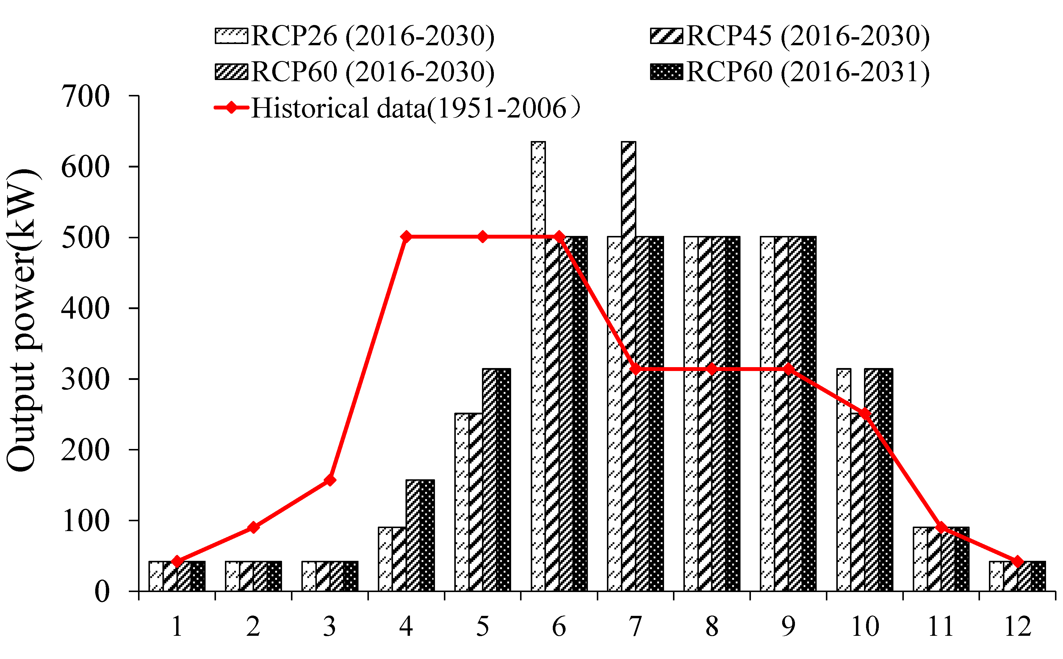
| 3. The results of this study clearly show the vulnerability of new energy systems to climate change. |
| 4. The findings also point to the wind energy potential associated with climate change. |
| Copula | |||
|---|---|---|---|
| Gumbel Copula | [1,∞) | ||
| Clayton Copula | (0,∞) | ||
| Frank Copula | R |
| Month | Wind Speed (m/s) |
|---|---|
| January | 4.20 |
| February | 4.24 |
| March | 6.21 |
| April | 8.92 |
| May | 9.08 |
| June | 8.52 |
| July | 8.37 |
| August | 8.38 |
| September | 7.88 |
| October | 6.51 |
| November | 5.17 |
| December | 4.14 |
| Approaches | Characteristic |
|---|---|
| MvCD | Simplicity of calculation; stochastic analysis; high dimensional problem-solving ability; nonlinear problem-solving ability; limited application scope |
| Artificial Neural Network, ANN | Strong distribution processing ability; distributed storage and learning ability; large parameter quantity requirement |
| Genetic Algorithm, GA | Simple analytical procedure; randomness; easy to combine with other algorithms; complex programming implementation; large parameter quantity requirement |
| Support Vector Machine, SVM | Generalization performance; high dimensional problem-solving ability; nonlinear problem solving ability; sensitive to missing data; no universal solution |
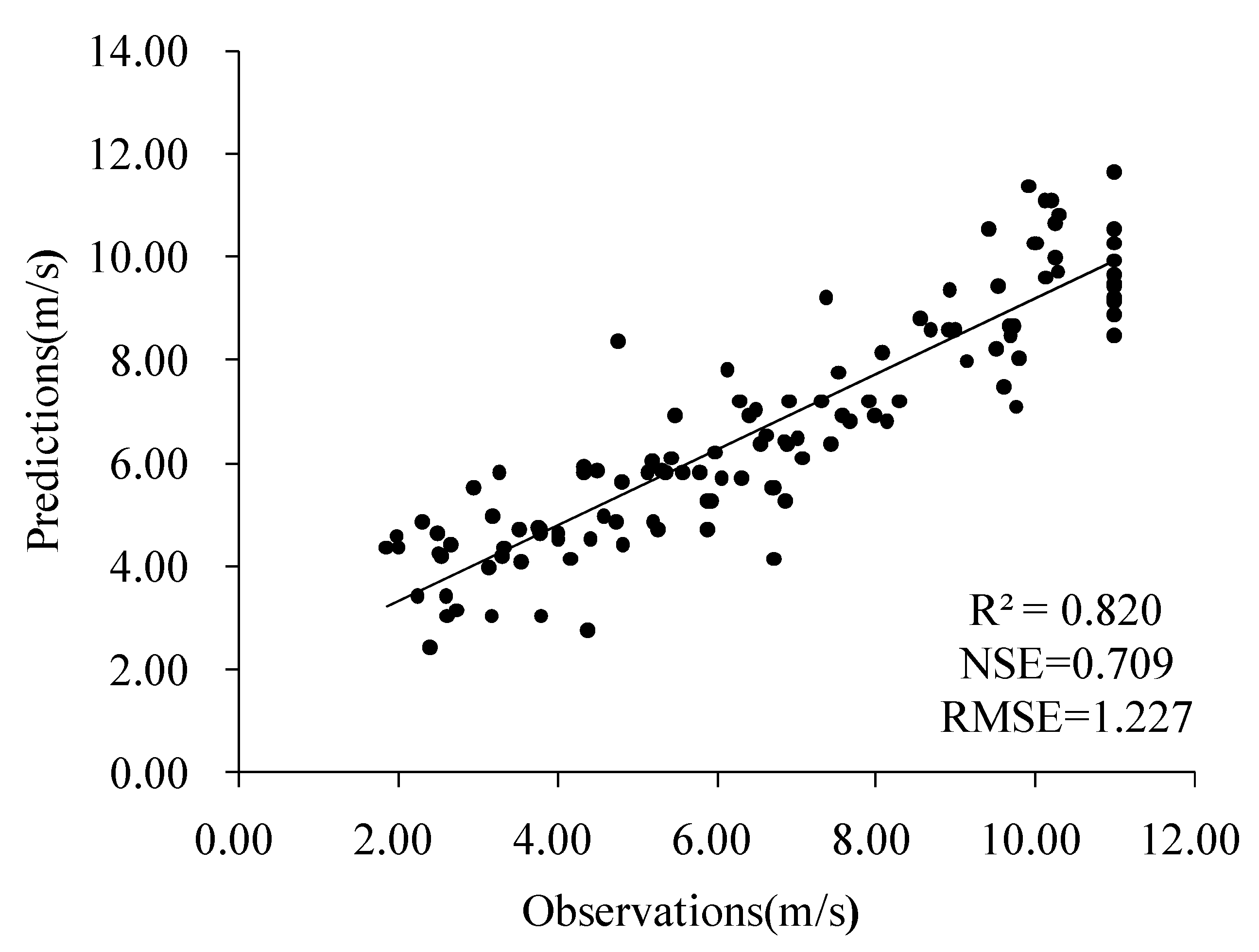
| Approaches | R2 | NSE | RMSE |
|---|---|---|---|
| MvCD | 0.82 | 0.709 | 1.227 |
| ANN | 0.85 | 0.34 | 3.234 |
| SVM | 0.771 | 0.826 | 4.17 |
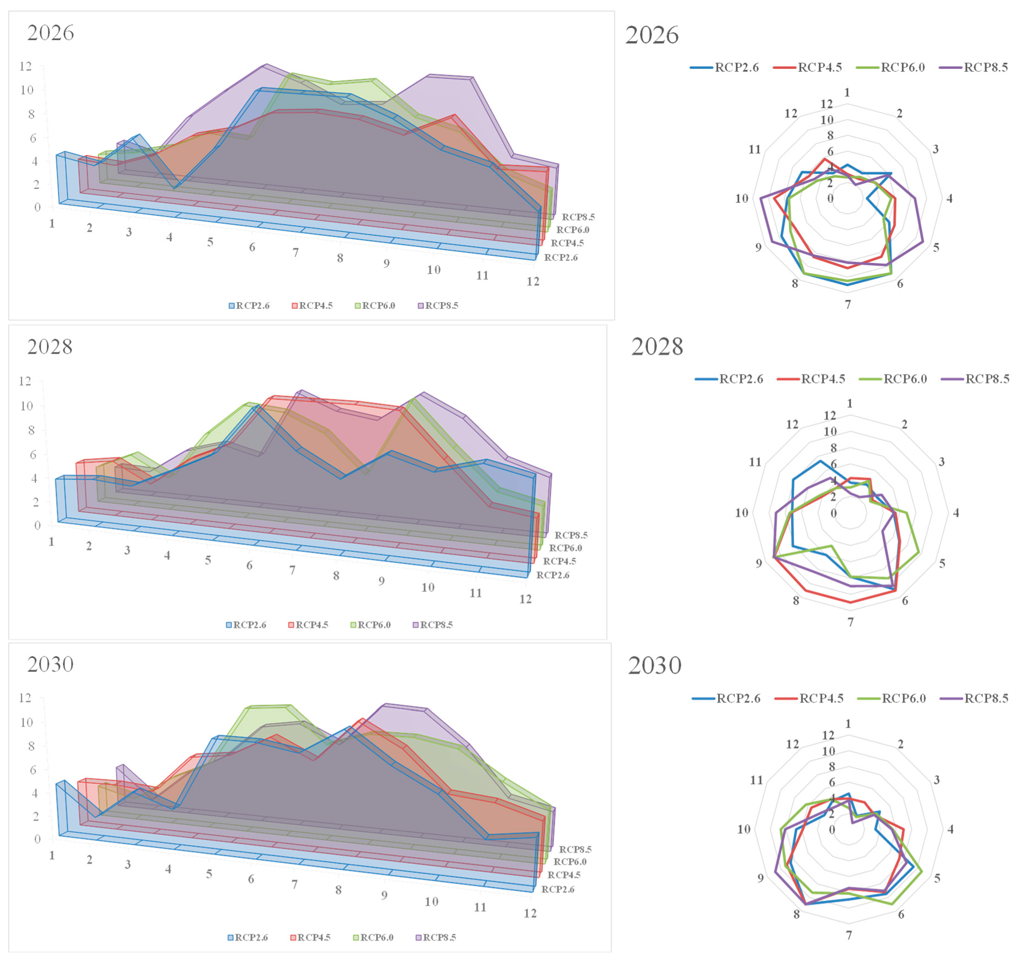
| 1 | 2 | 3 | 4 | 5 | 6 | 7 | 8 | 9 | 10 | 11 | 12 | ||
|---|---|---|---|---|---|---|---|---|---|---|---|---|---|
| 2016 | RCP2.6 | 6.12 | 4.04 | 5.19 | 4.59 | 7.39 | 9.62 | 11.00 | 9.48 | 8.43 | 10.23 | 2.58 | 4.51 |
| RCP4.5 | 5.11 | 3.87 | 3.61 | 5.79 | 7.37 | 9.41 | 10.63 | 11.00 | 6.58 | 8.52 | 3.41 | 3.22 | |
| RCP6.0 | 2.23 | 4.65 | 3.02 | 5.78 | 8.54 | 2.56 | 7.17 | 9.24 | 9.16 | 7.43 | 3.62 | 3.87 | |
| RCP8.5 | 3.47 | 4.49 | 3.95 | 5.16 | 6.52 | 11.00 | 8.88 | 7.93 | 11.00 | 8.39 | 5.25 | 2.52 | |
| 2020 | RCP2.6 | 2.93 | 3.89 | 3.20 | 5.46 | 8.16 | 10.32 | 6.63 | 7.48 | 10.82 | 9.65 | 4.45 | 2.17 |
| RCP4.5 | 3.71 | 3.69 | 3.13 | 5.23 | 8.03 | 11.00 | 10.19 | 7.64 | 11.00 | 7.26 | 6.03 | 4.55 | |
| RCP6.0 | 3.78 | 1.70 | 3.42 | 5.44 | 9.97 | 7.53 | 8.25 | 9.45 | 10.65 | 10.53 | 4.36 | 4.07 | |
| RCP8.5 | 3.46 | 3.81 | 3.85 | 5.79 | 6.89 | 8.65 | 9.04 | 8.75 | 10.75 | 8.27 | 3.21 | 5.55 | |
| 2030 | RCP2.6 | 4.55 | 1.98 | 4.53 | 3.39 | 9.50 | 9.48 | 8.90 | 11.00 | 8.55 | 6.69 | 3.60 | 4.16 |
| RCP4.5 | 3.91 | 3.98 | 3.71 | 6.97 | 7.42 | 9.19 | 7.56 | 11.00 | 9.10 | 5.85 | 5.51 | 4.44 | |
| RCP6.0 | 2.71 | 1.83 | 4.02 | 5.58 | 10.70 | 11.00 | 8.16 | 9.30 | 9.31 | 8.66 | 6.31 | 4.42 | |
| RCP8.5 | 3.67 | 0.93 | 3.71 | 5.46 | 8.48 | 9.03 | 7.45 | 11.00 | 10.81 | 8.09 | 4.14 | 3.34 |
Disclaimer/Publisher’s Note: The statements, opinions and data contained in all publications are solely those of the individual author(s) and contributor(s) and not of MDPI and/or the editor(s). MDPI and/or the editor(s) disclaim responsibility for any injury to people or property resulting from any ideas, methods, instructions or products referred to in the content. |
© 2025 by the authors. Licensee MDPI, Basel, Switzerland. This article is an open access article distributed under the terms and conditions of the Creative Commons Attribution (CC BY) license (https://creativecommons.org/licenses/by/4.0/).
Share and Cite
Wang, S.; Wu, J.; Lv, L. Impact of Climate Change on Wind Power Generation Studied Using Multivariate Copula Downscaling: A Case Study in Northwestern China. Energies 2025, 18, 1963. https://doi.org/10.3390/en18081963
Wang S, Wu J, Lv L. Impact of Climate Change on Wind Power Generation Studied Using Multivariate Copula Downscaling: A Case Study in Northwestern China. Energies. 2025; 18(8):1963. https://doi.org/10.3390/en18081963
Chicago/Turabian StyleWang, Shen, Jing Wu, and Lianhong Lv. 2025. "Impact of Climate Change on Wind Power Generation Studied Using Multivariate Copula Downscaling: A Case Study in Northwestern China" Energies 18, no. 8: 1963. https://doi.org/10.3390/en18081963
APA StyleWang, S., Wu, J., & Lv, L. (2025). Impact of Climate Change on Wind Power Generation Studied Using Multivariate Copula Downscaling: A Case Study in Northwestern China. Energies, 18(8), 1963. https://doi.org/10.3390/en18081963