Collaborative Planning of Source–Grid–Load–Storage Considering Wind and Photovoltaic Support Capabilities

Abstract

With the transformation of the global energy structure and the rapid development of new power generation technologies, new power system planning faces the challenge of multi-source–storage coordinated deployment. This paper proposes a new power system planning method, the collaborative planning of source–grid–load–storage, considering wind and photovoltaic power generation systems. First, taking into account the access of renewable energy such as wind and solar power, a renewable energy output model is constructed. Secondly, a typical intraday dispatch model of the new power system is constructed; on this basis, by adding constraints of different types of power sources, a multi-source and storage coordinated deployment planning model is constructed. Finally, through actual case studies in three provinces of Northeast China, the effectiveness of the proposed method is analyzed and verified. The results show that compared with traditional planning methods, the method proposed in this paper can significantly improve the economy and environmental friendliness of the system while meeting the requirements of power supply security.

1. Introduction

1.1. Background

The transition to new power generation systems is not merely a technological evolution but a fundamental change in how power is generated, transmitted, and consumed. As the global energy structure shifts towards renewable sources, the planning and operation of power systems must adapt to the multifaceted challenges of integrating new energy sources, such as solar and wind power, with traditional generation methods. The variability and uncertainty inherent in these new energy sources pose significant operational risks, leading to supply imbalances and increased system costs if not managed effectively. Since different energy forms are highly complementary in time and space, using a multi-source–storage complementary power generation method can effectively improve the power grid’s reliability [1]. Therefore, making full use of renewable energy sources such as wind and solar power to build a new power system planning method with multi-source–storage coordinated deployment is an important research direction.

Integrating new energy sources into the grid, especially the effective integration of renewable energy, such as wind and solar energy, has profoundly impacted the existing power system. First of all, the integration of new energy into the grid significantly reduces dependence on fossil fuels and reduces environmental pollution [2]. By using clean energy such as wind and solar energy, carbon emissions, and other air pollutants can be reduced, and the optimization of the energy structure can be promoted, which is crucial to achieving global emission reduction goals and combating climate change. Secondly, new energy grid connection technology provides technical support for the intelligent and sustainable development of the power system by improving its flexibility and stability. This improvement in flexibility is significant when a high proportion of new energy is penetrated. It is particularly important as it helps balance supply and demand, reduce energy waste, and improve energy efficiency [2]. However, if the use of new energy is unoptimized, it will also have some adverse effects on the power system. For example, integrating new energy into the grid may lead to declining power quality, including harmonic pollution, voltage fluctuations, and increased technical and economic risks [3]. These technical challenges need to be solved through scientific and reasonable measures to ensure the stable operation of the distribution network and improve the efficiency of using renewable energy power generation connected to the grid. As the proportion of renewable energy in the power grid increases, it also significantly impacts the safety and stability of the power system. A high proportion of variable renewable energy (VRE) may challenge the power system’s short-term flexibility and stability. The output of renewable energy, such as wind and solar power, is uncertain due to the variability in weather conditions. This uncertain volatility has had a huge impact on the long-term stability of the power system. Therefore, the accuracy of predictions for renewable energy needs to be improved further.

1.2. Literature Review

At present, scholars at home and abroad have conducted relevant research on the optimization planning of power systems with a high proportion of renewable energy. For the simulation of renewable energy output and the treatment of output uncertainty, Vallée et al. [4] and Borges and Dias [5] proposed a non-sequential Monte Carlo method, which directly performs multiple random samplings based on the wind speed distribution density function to generate a time series of wind speed. This method can ensure the distribution characteristics of wind speed but completely ignores the time series characteristics of wind speed. The wind speed time series obtained by this method cannot ensure that the intensity of wind speed changes is the same as the actual one. P. Chen et al. [6] proposed a time series ARIMA model method. This method first uses the ARIMA model to model the historical wind data and determine the parameters of the ARIMA model. Then, the obtained ARIMA model is used to generate the wind speed time series. This method considers the time series characteristics of wind speed and can simulate the severity of wind speed changes. However, this method does not consider the distribution characteristics of wind speed. The probability distribution of the obtained wind speed series cannot meet the expected typical wind speed distribution (such as the Weibull distribution). Verástegui et al. [7] proposed the idea of robust optimization to deal with this problem, but robust optimization often ignores the parameter information of renewable energy, resulting in overly conservative results. Liu C. et al. [8] proposed a random optimization method to deal with the uncertainty of renewable energy. Still, it requires specific distribution information on renewable energy, which is often difficult to obtain in real life. C. Zhao and Y. Guan [9] proposed using distributed robust optimization to deal with the uncertainty of new energy. However, since a large amount of historical data is required to form a data set, it increases the difficulty of planning. To improve the prediction accuracy of renewable energy output and reduce the uncertainty of renewable energy output, this paper proposes a stochastic difference equation method. Based on the theory of stochastic differential equations in random processes, this method considers the autocorrelation of wind speed time series and the probability distribution function of wind speed and analytically gives the stochastic differential equation of wind speed. After the stochastic differential equation is transformed into a stochastic difference equation, an iterative difference equation can generate the time series of wind speed. This method considers both the probability distribution of wind speed and the time series characteristics of wind speed. It can obtain a wind speed time series that conforms to the random characteristics of historical data, thereby improving the accuracy of wind power prediction.

To improve the power supply reliability problem of the power system, Suo et al. [10] established a new energy-wide-area complementary planning method for multi-energy power systems. It comprehensively considered the multi-energy complementary planning method in the time and space dimensions of new energy to improve the safe operation capability of the power grid. Z. Ren et al. [11] proposed a two-level planning model for tidal power farm (TCF) planning, which coordinates the micro-site selection strategy of tidal turbines (TCTs) and the collection system planning scheme to achieve a better balance between power generation, TCF capital investment, and the economic operation of the power system. Y. Fang et al. [12] proposes a novel expansion planning model with integrated operational flexibility constraints (EP-OFLX) that can effectively address long-term and short-term temporal variations and uncertainties and optimize investment decisions for generation and transmission facilities to achieve the desired level of renewable energy penetration. Z. Zhuo et al. [13] proposed an improved barrier method to effectively solve the coordination problem of renewable energy generation and other emerging power technologies in the low-carbon transformation of the power system. P. Han et al. [14] proposed a BESS power rating and capacity optimization method based on sequential production simulation technology to achieve the coordinated optimization of power and capacity of renewable energy battery energy storage systems. Z. Wen et al. [15] proposes an uncertainty modeling method based on the Wasserstein distance and Gaussian mixture model (W-GMM) to generate wind and solar energy scenarios to address RES-related uncertainties and promote low-carbon energy transformation. C. Lai and B. Kazemtabrizi [16] proposes a new tight constraint method to ensure the effectiveness of the day-ahead plan in real-time operation to improve the reliability of the day-ahead plan and ultimately to ensure the effectiveness of the day-ahead plan from the perspective of real-time operation. Guo et al. [17] proposes a hybrid system consisting of photovoltaic panels, air source heat pumps, batteries, and hot water tanks to meet the needs of the building. It develops a multi-objective, two-stage planning method to discover the optimal scheduling solution. Y. Tian et al. [18] proposes an HWPBS capacity planning framework that considers the characteristics of multi-energy grid connection to determine the optimal capacity configuration mode and scale of the hydropower–wind–solar–battery complementary system (HWPBS). Z. Yuan et al. [19] proposes a power system expansion planning model that integrates transmission expansion, renewable energy generation expansion, energy storage system deployment coordinated with coal-fired power plant retirement, and the transformation of coal-fired power plants into carbon capture plants to achieve the low-carbon transformation goals of the power industry. Z. Zhang et al. [20] proposed a planning method that considers the multi-temporal adequacy details of RES output and production time and demand differences to determine the size of short-term and seasonal energy storage and RES to achieve multi-temporal adequacy balance. However, most of the current literature tends to conduct the short-term planning of new power systems, and there is little research on the coordinated deployment of multiple sources and storage in new power systems and the annual planning problem (i.e., long-term planning).

Therefore, to deal with a series of power system security issues brought about by the grid connection of new energy systems and to formulate a long-term planning scheme for power systems that is both safe, economical, and environmentally friendly, this paper proposes a new power system planning method for multi-source–storage coordinated deployment. First, considering the access of new energy, a new energy output model was constructed; secondly, a typical intraday dispatch model including new energy was constructed; and finally, multi-source–storage coordinated deployment was achieved by adding constraints—the construction of planning models. This paper first constructs a typical intraday scheduling model that includes new energy sources and then builds a new planning model by continuously adding new constraints to complete the coordinated deployment of multiple sources and storage.

The structure of this paper is as follows. Section 2 summarizes the overall framework of the model constructed in this paper. Section 3 introduces the renewable energy output model and establishes a typical daily planning model for a new power system considering the coordinated deployment of multiple sources and storage. Section 4 forms the final model by adding different types of power supply constraints. The experimental setup and case studies are presented in Section 5. Finally, Section 6 concludes the paper.

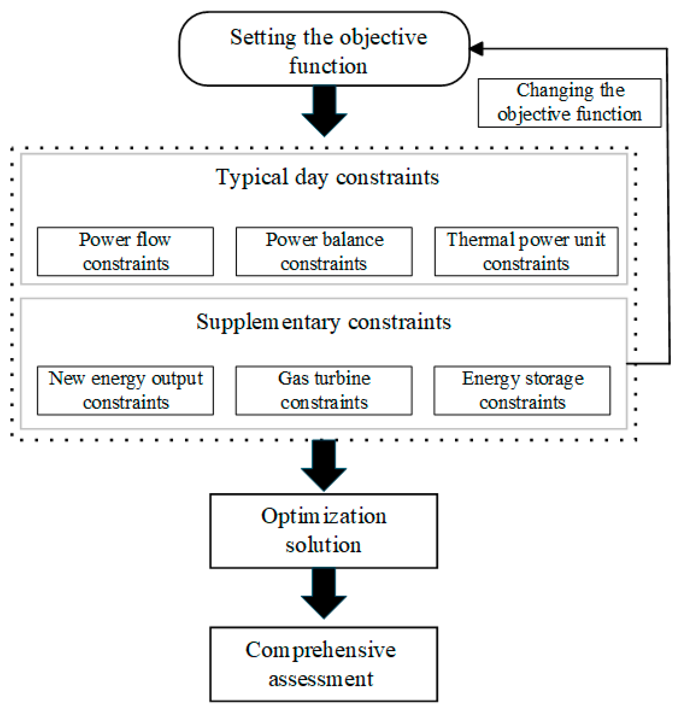
2. A New Power System Planning Framework Considering Multi-Source–Storage Coordinated Deployment

This paper designs a new power system planning method for multiple sources and storage combinations under different energy combinations by coordinating the deployment of different power sources and energy storage systems. The model takes the minimum economic cost as the goal and, on this basis, considers the optimal dispatching and operation modeling under different combinations and compares the advantages and disadvantages of different combinations. The planning framework is shown in Figure 1. First, using random difference equations and photovoltaic effects, we consider the analysis and modeling methods for constructing new energy output. Secondly, on this basis, we consider the planning modeling method of a typical day’s new power system dominated by thermal power units. Among them, with the goal of minimizing the total economic cost, the constraints within a typical day, including thermal power units, wind power, and photovoltaic energy, are considered, including minimum time start–stop constraints, thermal power unit climbing constraints, thermal power units and wind and solar output constraints, power balance constraints, flow constraints, etc., and we optimize the operation in the form of a typical day’s dispatch. Secondly, some thermal power units are replaced by gas turbine units to form a planning method for the coordinated scheduling of thermal power, gas turbine units, and renewable energy, and corresponding constraints are added, and the objective function is improved to optimize scheduling. Finally, the energy storage system is added to the plan, and a new power system with the coordinated deployment of multiple sources and storage is considered. Finally, corresponding conditions are added to form a planning method for optimized scheduling.

3. Construction of a New Power System Planning Model for Coordinated Deployment of Multiple Sources and Storage Based on Stochastic Difference Equations

This section considers the construction of a traditional combined new power system planning model. First, a traditional new power system planning model (including only thermal power units and renewable energy sources) is constructed. Second, different combination models are formed by adding different source and storage constraints. Finally, the results of different combination models are solved, and the advantages and disadvantages of different combinations are compared.

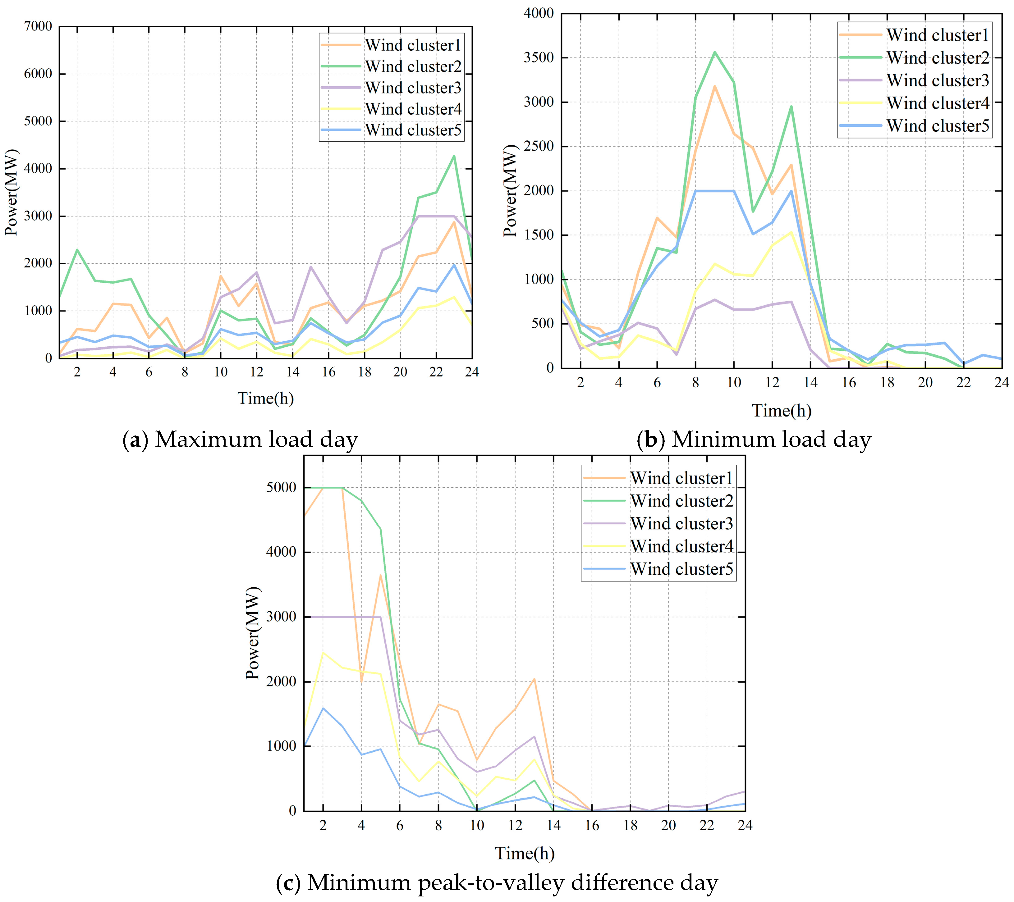
3.1. New Energy Output Analysis and Modeling

Renewable energy’s intermittent output may appear from 0 to its installed capacity. Therefore, the classic two-state model of conventional units cannot be used for the renewable energy reliability model. For this reason, this paper adopts a model that considers output timing. By considering various factors affecting the output of renewable energy, an analytical model is constructed to calculate the output of renewable energy [21].

a. Wind power output model

Considering the autocorrelation of the wind speed time series and the probability distribution function of the wind speed, the stochastic differential equation of the wind speed is obtained and then converted into a stochastic difference equation to generate the time series of the wind speed through iteration, and finally, the time series output of the wind farm is obtained. The specific method is as follows [22]:

Assume that the wind speed conforms to the Weibull distribution with scale parameters c and shape parameters k, respectively:

$$f(x)={\displaystyle \frac{k}{c}}{({\displaystyle \frac{x}{c}})}^{k-1}\exp [-{({\displaystyle \frac{x}{c}})}^k]$$

(1)

Then, the stochastic differential equation is obtained:

$$d{X}_t=-\theta (X_t-\mu )dt+\sqrt{v(X_t)}d{W}_t,t\ge 0$$

(2)

The average wind speed $E(x)=\mu =c\Gamma (1+{\displaystyle \frac{1}{k}})$, $\theta \ge 0$, $v(X_t)$ is defined as a non-negative function over the domain:

$$\begin{array}{ll}v(X_t)& ={\displaystyle \frac{2\theta }{f(x)}}{\displaystyle \int (\mu -x)f(x)dx}\\ & ={\displaystyle \frac{2\theta }{f(x)}}\left(c\Gamma (1+{\displaystyle \frac{1}{k}})\left(1-\exp \left[-{({\displaystyle \frac{x}{c}})}^k\right]\right)-c\Gamma \left({({\displaystyle \frac{x}{c}})}^k,1+{\displaystyle \frac{1}{k}}\right)\right)\\ \end{array}$$

(3)

Then,

$$\left\{\begin{array}{l}\Gamma (a)={\displaystyle {\int }_0^{+\infty }{y}^{a-1}{e}^{-y}}dy\\ \Gamma (x,a)={\displaystyle {\int }_0^x{y}^{a-1}{e}^{-y}}dy\end{array}\right.$$

(4)

In summary, the wind speed of a single wind farm is

$${\stackrel{⌢}{v}}_{w,t}={\stackrel{⌢}{v}}_{w,t-1}+d{X}_t$$

(5)

Affected by the climate, the wind speed levels in the areas where wind farms are located are different in different seasons (low in winter and high in summer), which has a certain regularity. In addition, the different surface temperatures during the day also affect the average wind speed at different times of the day (low in the day and high in the evening). Therefore, considering the seasonality and daily regularity of wind speed, the randomly generated wind speed sequence is corrected as follows [23]:

$$v_{w,t}=k_{w,m}{k}_{w,h}{\stackrel{⌢}{v}}_{w,t}$$

(6)

Considering the output characteristic curve of wind turbines, the wake effect of wind farms, and the output reliability of wind turbines in wind farms, the final wind farm timing output curve is as follows [24]:

$$P_{w,t}=n_t(1-{\eta }_w)C_w(v_{w,t})$$

(7)

Then,

$$C_w(v)=\left\{\begin{array}{ll}0,& 0\le v\le v_{in},v>v_{out}\\ {\displaystyle \frac{v^3-{v_{in}}^3}{{v_{out}}^3-{v_{in}}^3}}R,& 0\le v\le v_{rated}\\ R& v_{rated}\le v\le v_{out}\end{array}\right.$$

(8)

b. Photovoltaic output model

The basic principle of photovoltaic power generation is the photovoltaic effect, which uses solar panels to convert solar energy into electrical energy. The studies in [25] have shown that the output of solar panels at time t is

$$P_{v,t}=P_{stc}{\displaystyle \frac{I(R_t,k_t,I_{0t})}{I_{stc}}}[1+{\alpha }_t(T_t-T_{stc})]$$

(9)

Among them, $I(R_t,k_t,I_{0t})$ represents the total irradiance on the photovoltaic panel after considering factors such as solar irradiation, the clear sky index, and the photovoltaic panel tracking type; T represents the atmospheric temperature; $P_{stc}$, $T_{stc}$, $I_{stc}$ and ${\alpha }_t$ are all constants; and the factors that affect the output of the solar panel are $R_t,k_t,I_{0t},T$.

3.2. Objective Functions

This paper establishes an optimal dispatch model for the power system with the goal of minimizing the total system cost, as shown in Formula (10). The total system cost that needs to be considered includes the operating fuel consumption and start-stop fuel consumption of thermal power units, as well as the load shedding cost and various energy and energy storage costs.

$$C^{\mathit{Total}}=\min \left\{C_1+C_2+C_3\right\}$$

(10)

$$C_1={\displaystyle \sum _t{\displaystyle \sum _g\left\{d_{g,t}(a_g{P}_{g,t}^2+b_g{P}_{g,t}+c_g)+(C_g^{st}{d}_{g,t}^{on}+C_g^{sd}{d}_{g,t}^{off})\right\}}}$$

(11)

$$C_2=\beta L^{Total,cur}$$

(12)

$$C_3={\displaystyle \sum _t{\displaystyle \sum _{\Omega }\Omega {\lambda }_{\Omega }}}$$

(13)

Among them, $C_1$ represents the traditional planning cost, including the typical daily operation cost and start-up and shutdown cost of the unit; $a_g$, $b_g$, and $c_g$ represent the coal consumption coefficient of the unit, respectively; $C_g^{st}$ and $C_g^{sd}$ represent the start-up and shutdown costs of the unit, respectively; $d_{g,t}^{on}$ and $d_{g,t}^{off}$ represent the start-up and shutdown status of the unit, respectively; $C_2$ represents the load shedding cost of the unit; $\beta$ represents the load shedding cost coefficient; $L^{Total,cur}$ represents the total load shedding amount; $C_3$ represents the cost incurred when considering different energy sources and energy storage; ${\lambda }_{\Omega }$ represents the cost coefficient of different units; and $\Omega$ represents the total load shedding cost of the unit, $\Omega =\left\{G,W,V,E\right\}$.

3.3. Typical Day Constraints

The model constructed in this section only considers typical intraday constraints, including thermal power unit ramp constraints, minimum start and stop time constraints, output constraints, operation reserve constraints, power flow constraints, wind power and photovoltaic output constraints as follows:

a. Thermal power unit constraints

$$\left\{\begin{array}{l}{T}_{g,t\in T_t^{{\rm X}}}^{on}={\stackrel{⌢}{d}}_{g,t\in T_t^{{\rm X}}}{T}_{g,t-1\in T_t^{{\rm X}}}^{on}+{\stackrel{⌢}{d}}_{g,t\in T_t^{{\rm X}}}\\ T_{g,t\in T_t^{{\rm X}}}^{off}=T_{g,t-1\in T_t^{{\rm X}}}^{off}(1-{\stackrel{⌢}{d}}_{g,t\in T_t^{{\rm X}}})+(1-{\stackrel{⌢}{d}}_{g,t\in T_t^{{\rm X}}})\\ ({\stackrel{⌢}{d}}_{g,t\in T_t^{{\rm X}}}-{\stackrel{⌢}{d}}_{g,t-1\in T_t^{{\rm X}}})(T_{g,t-1\in T_t^{{\rm X}}}^{off}-T_g^{off})\ge 0\\ ({\stackrel{⌢}{d}}_{g,t-1\in T_t^{{\rm X}}}-{\stackrel{⌢}{d}}_{g,t\in T_t^{{\rm X}}})(T_{g,t-1\in T_t^{{\rm X}}}^{on}-T_g^{on})\ge 0\end{array}\right.$$

(14)

$$\left\{\begin{array}{l}(P_{g,t\in T_t^{{\rm X}}}+r_{g,t\in T_t^{{\rm X}}}^{up})-(P_{g,t-1\in T_t^{{\rm X}}}-r_{g,t-1\in T_t^{{\rm X}}}^{down})\le R_g^u\\ (P_{g,t\in T_t^{{\rm X}}}+r_{g,t-1\in T_t^{{\rm X}}}^{up})-(P_{g,t\in T_t^{{\rm X}}}-r_{g,t\in T_t^{{\rm X}}}^{down})\le R_g^d\end{array}\right.$$

(15)

$${\stackrel{⌢}{d}}_{g,t\in T_t^{{\rm X}}}{P}_g^{\min }+r_{g,t\in T_t^{{\rm X}}}^{down}\le P_{g,t\in T_t^{{\rm X}}}\le {\stackrel{⌢}{d}}_{g,t\in T_t^{{\rm X}}}{P}_g^{\max }-r_{g,t\in T_t^{{\rm X}}}^{up}$$

(16)

Equations (14)–(16) represent the minimum start–stop time constraint, climbing constraint, and output constraint, respectively. $T_{g,t}^{on}$ represents the duration for which the thermal power unit has been continuously operating at time t; $T_{g,t}^{off}$ represents the duration for which the thermal power unit has been continuously offline at time t; $T_g^{on}$ represents the minimum start-up time for the thermal power unit; and $T_g^{off}$ represents the minimum shutdown time for the thermal power unit. $P_g^{\min }$ and $P_g^{\max }$ represent the upper and lower limits of the thermal power unit’s output, respectively; $P_{g,t}$ represents the planned production of the thermal power unit at time t; and $R_g^u$, $R_g^d$ represent the ramp-up and ramp-down rates of the thermal power unit, respectively. Equation (24) represents the output constraints for the thermal power unit, and $r_{g,t}^{up}$ and $r_{g,t}^{down}$ represent the upper and lower limits of the thermal power unit’s reserve capacity.

b. Intraday power balance constraints

The typical day is $X=\left\{A,B,C,D\dots \right\}$. The power balance constraints of each typical day are constructed as follows:

$${\displaystyle \sum _{g\in {\Omega }_i^G}{P}_{g,t\in T_t^{{\rm X}}}}+{\displaystyle \sum _{w\in {\Omega }_i^W}{P}_{w,t\in T_t^{{\rm X}}}}+{\displaystyle \sum _{v\in {\Omega }_i^V}{P}_{v,t\in T_t^{{\rm X}}}}={\displaystyle \sum _{j\in {\Omega }_i^J}{P}_{ij,t\in T_t^{{\rm X}}}}+L_{i,t\in T_t^{{\rm X}}}-L_{i,t\in T_t^{{\rm X}}}^{cur}$$

(17)

Quantitative indicators of supply and demand balance on a typical day are as follows:

$$L^{X,cur}={\displaystyle \sum _i{\displaystyle \sum _t{L}_{i,t\in T_t^{{\rm X}}}^{cur}}}$$

(18)

Among them, ${\Omega }_i^G$, ${\Omega }_i^W$, and ${\Omega }_i^V$ represent the sets of different types of units belonging to node i and ${\Omega }_i^J$ represents the set of nodes connected to node i.

c. Intraday power constraints

$$\left\{\begin{array}{l}{P}_{ij,t\in T_t^{{\rm X}}}={\displaystyle \frac{{\delta }_i-{\delta }_j}{x_{ij}}}\\ P_{ij,t\in T_t^{{\rm X}}}^{\min }\le P_{ij,t\in T_t^{{\rm X}}}\le P_{ij,t\in T_t^{{\rm X}}}^{\max }\\ -\pi /2\le {\delta }_i,{\delta }_j\le \pi /2\end{array}\right.$$

(19)

where ${\delta }_i$ and ${\delta }_j$ represent the power angles at nodes $i$ and $j$, respectively and $x_{ij}$ represents the impedance between nodes $i$ and $j$.

d. Renewable energy output constraints

$$\left\{\begin{array}{l}0\le P_{w,t\in T_t^{{\rm X}}}\le U_w{\Theta }_{w,t\in T_t^{{\rm X}}}\\ P_{w,t\in T_t^{{\rm X}}}+P_{w,t\in T_t^{{\rm X}}}^{cur}=U_w{\Theta }_{w,t\in T_t^{{\rm X}}}\end{array}\right.$$

(20)

$$\left\{\begin{array}{l}0\le P_{v,t\in T_t^{{\rm X}}}\le U_v{\Theta }_{v,t\in T_t^{{\rm X}}}\\ P_{v,t\in T_t^{{\rm X}}}+P_{v,t\in T_t^{{\rm X}}}^{cur}=U_v{\Theta }_{v,t\in T_t^{{\rm X}}}\end{array}\right.$$

(21)

Formulas (20) and (21) represent the upper and lower output constraints of wind power and photovoltaic power, respectively.

4. Multi-Source–Storage Coordinated Deployment Analysis and Modeling

To realize the modeling of planning methods with different combinations, we add different constraints to the original model and change the objective function. By adding different constraints and objective functions, the safety and reliability of the optimized operation of the new power system planning methods with different combinations can be guaranteed, thereby realizing planning schemes with different combinations.

4.1. Gas Turbine Plant Modeling

Consider adding gas turbine planning and adding gas turbine costs [26,27]:

$$C_{GT}={\displaystyle \frac{3600c}{\eta D(1-y)}}$$

(22)

Modify the original constraint condition (17) as follows:

$${\displaystyle \sum _{g\in {\Omega }_i^G}{P}_{g,t\in T_t^{{\rm X}}}}+{\displaystyle \sum _{gt\in {\Omega }_i^{GT}}{P}_{gt,t\in T_t^{{\rm X}}}}+{\displaystyle \sum _{w\in {\Omega }_i^W}{P}_{w,t\in T_t^{{\rm X}}}}+{\displaystyle \sum _{v\in {\Omega }_i^V}{P}_{v,t\in T_t^{{\rm X}}}}={\displaystyle \sum _{j\in {\Omega }_i^J}{P}_{ij,t\in T_t^{{\rm X}}}}+L_{i,t\in T_t^{{\rm X}}}-L_{i,t\in T_t^{{\rm X}}}^{cur}$$

(23)

$$P_{gt,t\in T_t^{{\rm X}}}=\eta Q_{t\in T_t^{{\rm X}}}D$$

(24)

4.2. Energy Storage Modeling

Considering the addition of energy storage to the planning, it is necessary to modify the original constraint Formula (17) and add energy storage constraints [28]:

$$\begin{array}{l}{\displaystyle \sum _{g\in {\Omega }_i^G}{P}_{g,t\in T_t^{{\rm X}}}}+{\displaystyle \sum _{w\in {\Omega }_i^W}{P}_{w,t\in T_t^{{\rm X}}}}+{\displaystyle \sum _{v\in {\Omega }_i^V}{P}_{v,t\in T_t^{{\rm X}}}}+{\displaystyle \sum _{s\in {\Omega }_i^S}(E_{s,t\in T_t^{{\rm X}}}^{dis}-}{E}_{s,t\in T_t^{{\rm X}}}^{cha})=\\ {\displaystyle \sum _{j\in {\Omega }_i^J}{P}_{ij,t\in T_t^{{\rm X}}}}+L_{i,t\in T_t^{{\rm X}}}-L_{i,t\in T_t^{{\rm X}}}^{cur}\end{array}$$

(25)

$$S_{s,t\in T_t^{{\rm X}}}=S_{s,t-1\in T_t^{{\rm X}}}+{\eta }_s^{cha}{E}_{s,t\in T_t^{{\rm X}}}^{cha}-E_{s,t\in T_t^{{\rm X}}}^{dis}/{\eta }_s^{dis}$$

(26)

$$\begin{array}{l}0\le E_{s,t\in T_t^{{\rm X}}}^{cha},E_{s,t\in T_t^{{\rm X}}}^{dis}\le U_{s}T{D}_{T_t^{{\rm X}}}\\ 0\le S_{s,t\in T_t^{{\rm X}}}\le U_{s}T\\ S_{s,t_0}=S_{s,t_{24}}\end{array}$$

(27)

As shown in Figure 2, the analysis and solution process of the optimization model in this paper is given. First, considering the typical intra-day constraints, a traditional optimization scheduling model is constructed. Secondly, when performing different combination planning, corresponding constraints and target costs are added. Finally, according to different planning schemes, the optimization results are solved and compared and analyzed.

5. Case Analysis

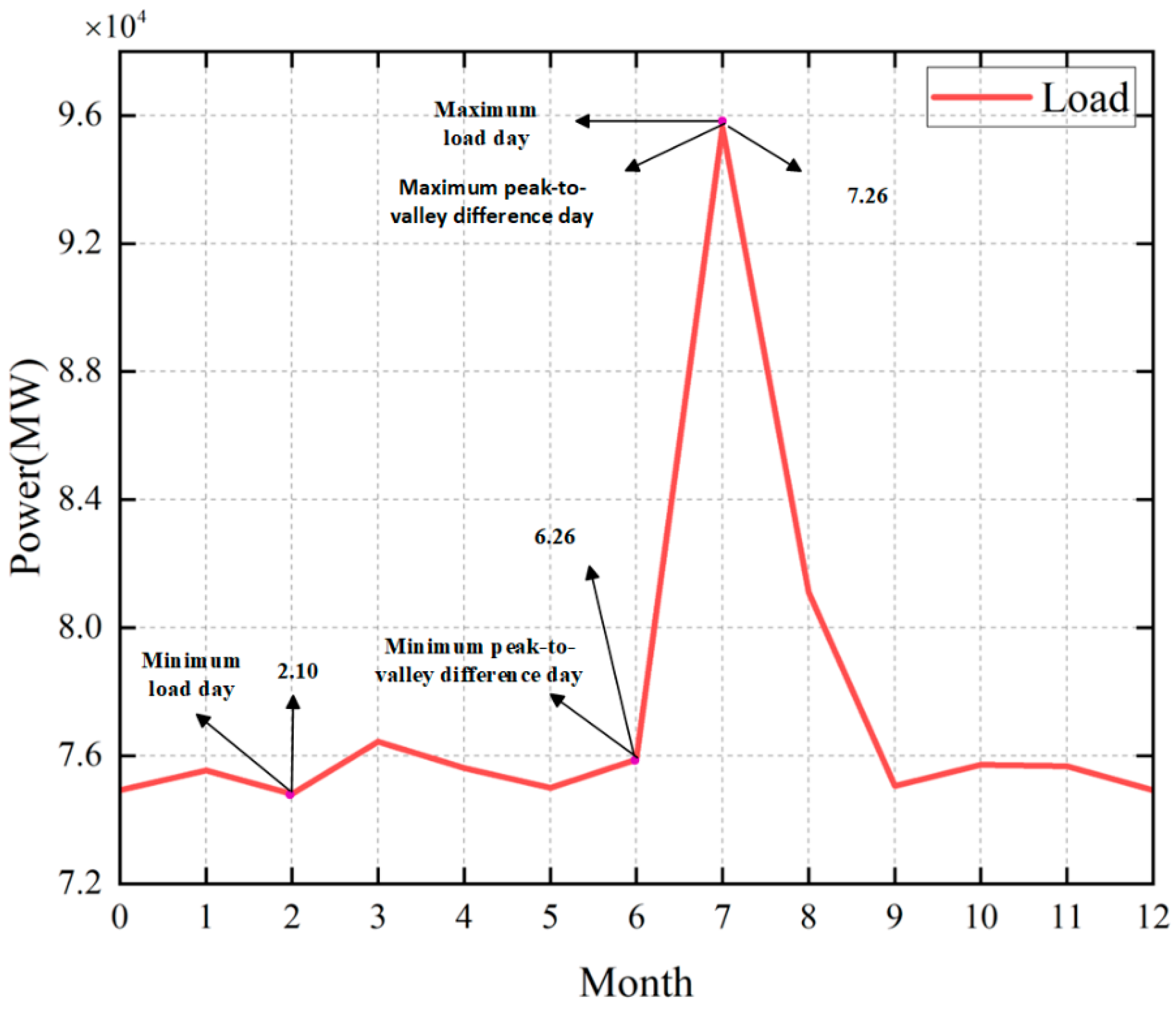
5.1. Data Description and Simulation Setup

This paper selects a 145-node system in a specific area of the three northeastern provinces for research to compare the advantages and disadvantages of new power system planning methods with different combinations of collaborative optimization. The relevant data come from the actual data of the power grid in the three northeastern provinces in 2024. By selecting different combinations to establish a planning method, the constructed optimization model solves directly using a commercial solver, such as Gurobi.

The schemes set in this paper are shown in

Table 1. Unit deployment plan.

Number of Units	Case 1	Case 2	Case 3	Case 4
$N_G$	135	120	127	112
$N_{GT}$	0	15	0	15
$N_E$	0	0	8	8
$N_W$	5	5	5	5
$N_V$	5	5	5	5

below:

Case 1: Select only thermal power units and renewable energy as power supply energy to construct an optimization model;

Case 2: Select thermal power units, gas turbine units, and renewable energy as power supply energy to construct an optimization model;

Case 3: Select thermal power units and renewable energy as power supply energy to construct an optimization model and add energy storage devices;

Case 4: Select thermal power units, gas turbine units, and renewable energy as power supply energy to construct an optimization model and add energy storage devices.

Figure 3 shows the typical days selected in this paper. As shown in the figure, this paper selects the minimum load day, maximum load day, minimum peak-to-valley difference day, and maximum peak-to-valley difference day (the maximum load day and the maximum peak-to-valley difference day are the same day). This paper selects these typical days for case analysis.

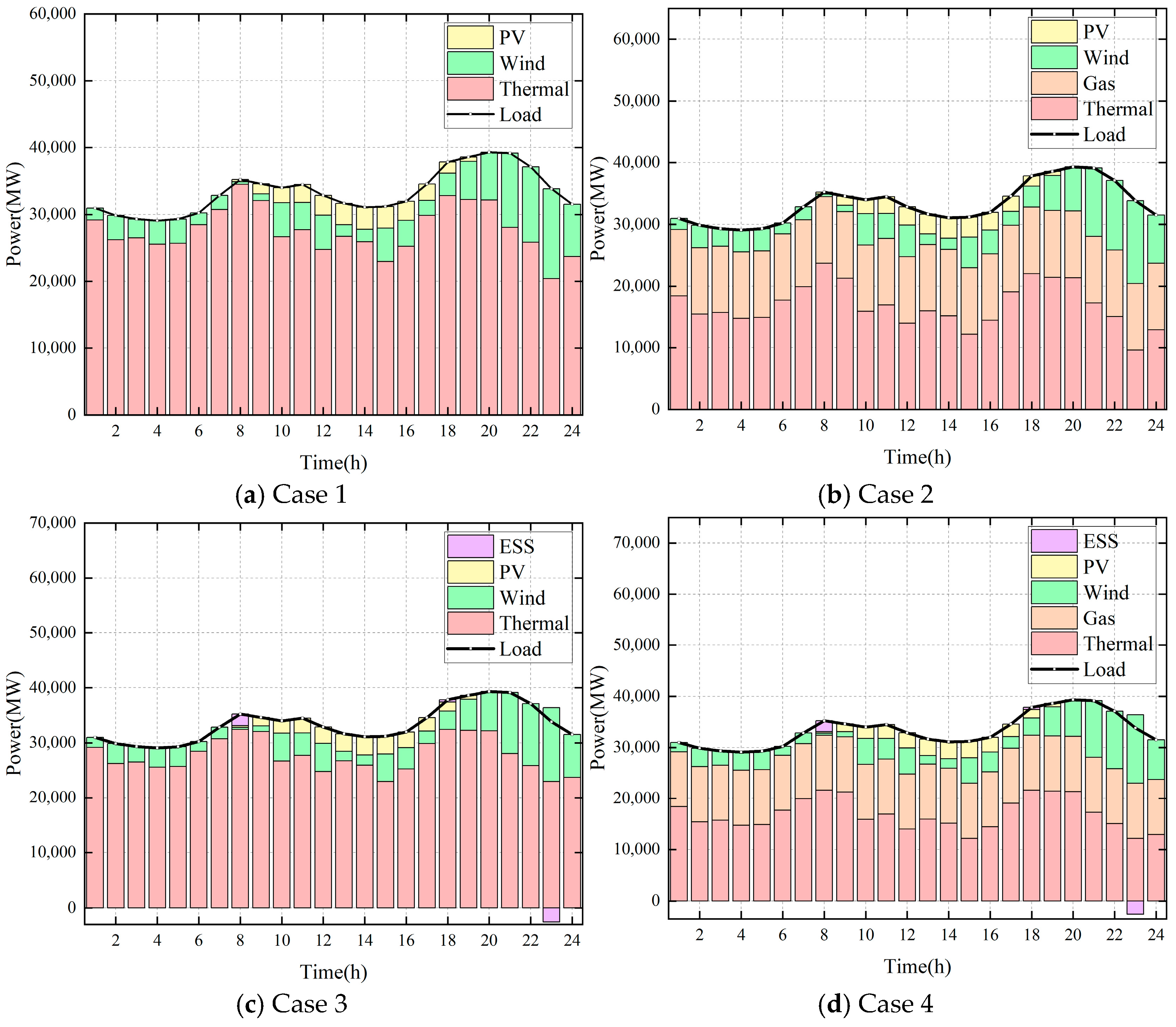
5.2. Power Supply-Related Statistics

a. New energy output

Figure 4 shows the output of five wind clusters on the minimum load day, maximum load day, and the day with the smallest peak-to-valley difference. It can be seen from the figure that the output of each wind cluster is different under different load conditions. The output trends of each wind farm on the same day are similar. On the maximum load day, the output of each wind farm shows a concave trend; on the minimum load day, the output of each wind farm shows a trend of being obvious in the middle and smaller on both sides; on the day with the smallest peak-to-valley difference, the output of each wind farm gradually decreases over time.

Figure 5 shows the output of five PV clusters on the minimum load day, maximum load day, and the day with the smallest peak-to-valley difference. The output trends of the PV clusters are basically similar, showing a trend of being large in the middle and small on both sides. The output is mainly concentrated from 8 a.m. to 8 p.m.

b. Number of starts and stops of thermal power units

Figure 6 shows the number of starts and stops of thermal power units under different schemes throughout the year. It can be seen from the figure that the units in Schemes 1 and 2 have the highest number of starts and stops; when energy storage devices are added, the number of starts and stops of thermal power units in Schemes 3 and 4 decreases significantly.

5.3. Economic Analysis

Figure 7 shows a bar chart comparing the total costs obtained under different allocation schemes. The figure clearly shows that the total cost of Example 1 is the highest, and the total cost of Example 4 is the lowest; that is, the traditional planning method is the worst in terms of economic efficiency, and the multi-source–storage system planning and scheduling is the best in terms of economic efficiency.

Table 2. Cost summary of different cases.

Cost ($\times {10}^9$ yuan)	Case 1	Case 2	Case 3	Case 4
$C_G$	1686.78	1392.85	1685.70	1391.25
$C_{GT}$	0.00	45.88	0.00	45.00
$C_W$	46.80	46.80	46.80	46.80
$C_V$	10.40	10.40	10.40	10.40
$C_E$	0.00	0.00	16.00	16.00
$C_{Cur}$	1243.50	585.56	0.00	0.00

shows various costs under different examples. Examples 1 and 2 incur load shedding costs, with Example 1 having the highest cost. Examples 3 and 4 do not incur load shedding costs, with Example 4 having the lowest cost.

5.4. Supply and Demand Balance Analysis

Figure 8 shows the output of the units under different calculation cases on the minimum load day. It can be seen from the figure that in Example 1, the load power supply is basically borne by the thermal power units; in Example 2, the load power supply is borne by the thermal power units and the gas turbine units; on the minimum load day, in Example 3, the energy storage basically does not participate in the output, and the thermal power units mainly bear the power supply; and similarly, on the minimum load day, in Example 4, the energy storage basically does not participate in the output, and the thermal power units and the gas turbine units mainly bear the load power supply.

Figure 9 shows the output of the units under different calculation cases on the maximum load day. It can be seen from the figure that on the maximum load day, in Example 1, the load power supply is borne by the thermal power units, but it cannot meet the load supply at all times. At 12 and 14 o’clock, many load shedding situations occur; in Example 2, the load power supply is borne by the thermal power units and gas turbine units, which also cannot meet the load supply at all times. At 12 and 14 o’clock, a small amount of load shedding situations occur; in Examples 3 and 4, the load supply is guaranteed due to energy storage participation, and the system load shedding problem is solved.

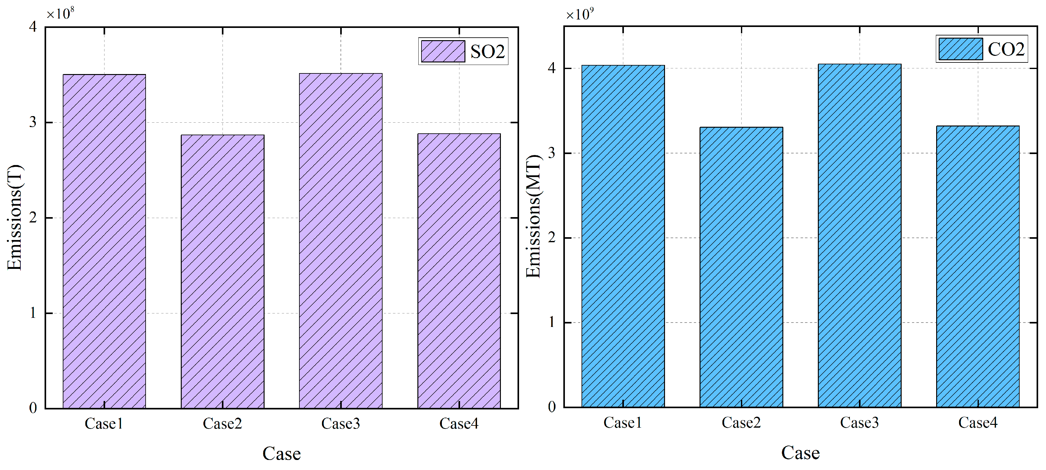
5.5. Environmental Analysis

As shown in Figure 10, the emissions of carbon dioxide and sulfur dioxide under different schemes are displayed. It can be seen from the figure that the carbon dioxide and sulfur dioxide emissions of Scheme 1 and Scheme 3 are greater than those of Scheme 2 and Scheme 4; that is, when Scheme 1 and Scheme 3 are used, the degree of environmental pollution is higher. Additionally, when the gas units are involved in the scheduling, that is, using Scheme 2 and Scheme 4 for scheduling, it has a significant effect on reducing the degree of environmental pollution.

6. Conclusions

To avoid the impact of high-proportion renewable energy grid connection on the safety and reliability of the power system and improve the economic efficiency and environmental impacts of the power grid, a new power system planning method with multi-source–storage coordinated dispatch is proposed. It is proposed that stochastic difference equations and the photovoltaic effect be used to simulate renewable energy output. Then, a new power system annual planning scheme based on a typical day’s dispatch is constructed by adding source–storage-related constraints. The numerical results show that the proposed method can reduce the degree of system load shedding and improve the system’s economic efficiency, safety, and environmental impacts. The main contributions of this paper are as follows:

(1) This paper proposes a wind farm operation simulation model based on stochastic difference equations, which takes into account both the probability distribution of wind speed and the time series characteristics of wind speed and can obtain a wind speed time series that conforms to the random characteristics of historical data;

(2) This paper takes daily dispatch as the core and uses the typical day analysis method to optimize and evaluate the planning method of the new power system throughout the year;

(3) The new power system planning method of multi-source–storage coordinated deployment proposed in this paper comprehensively quantifies and examines the safety, economic efficiency, and environmental protection of the power system.

The new power system planning method with multi-source–storage coordinated dispatch effectively improves the anti-interference ability of the power system under the condition of high-proportion renewable energy grid connection. On the one hand, it incorporates a variety of energy sources and energy storage devices. This is conducive to ensuring the safety of power system dispatch. It makes up for the lack of complementary capabilities of traditional dispatch methods, thereby alleviating related safety defects. On the other hand, compared with traditional dispatch, it reduces the cost of power system dispatch while ensuring the safe operation of the power system. It also improves the environmental protection performance of the system. In the future, we can further study the coordinated dispatch strategies between different types of energy to improve the flexibility and adaptability of the system. At the same time, it is possible to consider conducting relevant research under extreme weather conditions and respond to the impact of extreme weather and emergencies on the operation of the power system through the coordinated optimization of multiple sources and storage.

References

1. Numan, M.; Baig, M.F.; Yousif, M. Reliability evaluation of energy storage systems combined with other grid flexibility options: A review. J. Energy Storage 2023, 63, 107022. [Google Scholar]
2. Harrouz, A.; Abbes, M.; Colak, I.; Kayisli, K. Smart grid and renewable energy in Algeria. In Proceedings of the 2017 IEEE 6th International Conference on Renewable Energy Research and Applications (ICRERA), San Diego, CA, USA, 5–8 November 2017; pp. 1166–1171. [Google Scholar]
3. Li, Y.; Liu, H.; Fan, Y.; Tian, X.; Xiao, Y.; Wang, C. Research on the Technology Requirement of Distributed Renewable Energy AC/DC Output System and Network Voltage Coordinated Control. In Proceedings of the 2020 IEEE 4th Conference on Energy Internet and Energy System Integration (EI2), Wuhan, China, 30 October–1 November 2020; pp. 2369–2372. [Google Scholar]
4. Vallée, F.; Brunieau, G.; Pirlot, M.; Deblecker, O.; Lobry, J. Optimal wind clustering methodology for electrical network adequacy studies using non sequential Monte Carlo simulation. In Proceedings of the 2011 International Conference on Clean Electrical Power (ICCEP), Ischia, Italy, 14–16 June 2011; pp. 778–785. [Google Scholar]
5. Borges, C.L.T.; Dias, J.A.S. A Model to Represent Correlated Time Series in Reliability Evaluation by Non-Sequential Monte Carlo Simulation. IEEE Trans. Power Syst. 2017, 32, 1511–1519. [Google Scholar] [CrossRef]
6. Chen, P.; Pedersen, T.; Bak-Jensen, B.; Chen, Z. ARIMA-Based Time Series Model of Stochastic Wind Power Generation. IEEE Trans. Power Syst. 2010, 25, 667–676. [Google Scholar] [CrossRef]
7. Verástegui, F.; Lorca, Á.; Olivares, D.E.; Negrete-Pincetic, M.; Gazmuri, P. An Adaptive Robust Optimization Model for Power Systems Planning With Operational Uncertainty. IEEE Trans. Power Syst. 2019, 34, 4606–4616. [Google Scholar] [CrossRef]
8. Liu, C.; Lee, C.; Chen, H.; Mehrotra, S. Stochastic robust mathematical programming model for power system optimization. IEEE Trans. Power Syst. 2015, 31, 821–822. [Google Scholar] [CrossRef]
9. Zhao, C.; Guan, Y. Data-Driven Stochastic Unit Commitment for Integrating Wind Generation. IEEE Trans. Power Syst. 2016, 31, 2587–2596. [Google Scholar] [CrossRef]
10. Suo, X.; Zhao, S.; Ma, Y.; Dong, L. New Energy Wide Area Complementary Planning Method for Multi-Energy Power System. IEEE Access 2021, 9, 157295–157305. [Google Scholar] [CrossRef]
11. Ren, Z.; Wang, Y.; Li, H.; Liu, X.; Wen, Y.; Li, W. A Coordinated Planning Method for Micrositing of Tidal Current Turbines and Collector System Optimization in Tidal Current Farms. IEEE Trans. Power Syst. 2019, 34, 292–302. [Google Scholar] [CrossRef]
12. Fang, Y.; Han, J.; Du, E.; Jiang, H.; Fang, Y.; Zhang, N.; Kang, C. Electric energy system planning considering chronological renewable generation variability and uncertainty. Appl. Energy 2024, 373, 123961. [Google Scholar] [CrossRef]
13. Zhuo, Z.; Zhang, N.; Hou, Q.; Du, E.; Kang, C. Backcasting Technical and Policy Targets for Constructing Low-Carbon Power Systems. IEEE Trans. Power Syst. 2022, 37, 4896–4911. [Google Scholar] [CrossRef]
14. Han, P.; Li, P.; Xie, X.; Zhang, J. Coordinated Optimization of Power Rating and Capacity of Battery Storage Energy System with Large-Scale Renewable Energy. In Proceedings of the 2022 IEEE 6th Conference on Energy Internet and Energy System Integration (EI2), Chengdu, China, 28–30 October 2022; pp. 189–193. [Google Scholar]
15. Wen, Z.; Zhang, X.; Wang, H.; Wang, G.; Wu, T.; Qiu, J. Low-carbon planning for integrated power-gas-hydrogen system with Wasserstein-distance based scenario generation method. Energy 2025, 316, 134388. [Google Scholar] [CrossRef]
16. Lai, C.; Kazemtabrizi, B. A novel data-driven tighten-constraint method for wind-hydro hybrid power system to improve day-ahead plan performance in real-time operation. Appl. Energy 2024, 371, 123616. [Google Scholar] [CrossRef]
17. Guo, S.; Ren, F.; Wei, Z.; Zhai, X. A multi-objective collaborative planning method for a PV-powered hybrid energy system considering source-load matching. Energy Convers. Manag. 2024, 316, 118848. [Google Scholar] [CrossRef]
18. Tian, Y.; Chang, J.; Wang, Y.; Wang, X.; Meng, X.; Guo, A. The capacity planning method for a hydro-wind-PV-battery complementary system considering the characteristics of multi-energy integration into power grid. J. Clean. Prod. 2024, 446, 141292. [Google Scholar] [CrossRef]
19. Yuan, Z.; Zhang, H.; Cheng, H.; Zhang, S.; Zhang, X.; Lu, J. Low-carbon oriented power system expansion planning considering the long-term uncertainties of transition tasks. Energy 2024, 307, 132759. [Google Scholar] [CrossRef]
20. Zhang, Z.; Guo, Z.; Zhou, M.; Wu, Z.; Yuan, B.; Chen, Y.; Li, G. Equalizing multi-temporal scale adequacy for low carbon power systems by co-planning short-term and seasonal energy storage. J. Energy Storage 2024, 84, 111518. [Google Scholar] [CrossRef]
21. Wei, H.; Ma, M.; Jiang, H.; Capuder, T.; Teng, F.; Strbac, G.; Zhang, J.; Zhang, N.; Kang, C. Generation and transmission expansion planning incorporating economically feasible heterogeneous demand-side resources. Appl. Energy 2025, 381, 125067. [Google Scholar] [CrossRef]
22. Zhang, Y.; Zhao, Y. Research on Wind Power Prediction Based on Time Series. In Proceedings of the 2021 IEEE International Conference on Artificial Intelligence and Industrial Design (AIID), Guangzhou, China, 28–30 May 2021; pp. 78–82. [Google Scholar]
23. Wang, K.; Zou, J.; Lu, S.; Wang, J.; Zhou, B. Wind Power Output Scene Reconstruction Method Considering Wind Speed Autocorrelation and Source Load Cross-Correlation. In Proceedings of the 2022 5th International Conference on Power and Energy Applications (ICPEA), Guangzhou, China, 18–20 November 2022; pp. 687–692. [Google Scholar]
24. Teng, Y.; Xu, J.; Zhang, M.; Liang, W. Study of wind farm power output predicting model based on nonlinear time series. In Proceedings of the 2011 International Conference on Electrical Machines and Systems, Beijing, China, 20–23 August 2011; pp. 1–4. [Google Scholar]
25. Cheng, Y.; Zhang, N.; Lu, Z.; Kang, C. Planning multiple energy systems toward low-carbon society: A decentralized approach. IEEE Trans. Smart Grid 2018, 10, 4859–4869. [Google Scholar] [CrossRef]
26. Wang, C.; Zhang, R.; Bi, T. Energy management of distribution-level integrated electric-gas systems with fast frequency reserve. IEEE Trans. Power Syst. 2023, 39, 4208–4223. [Google Scholar] [CrossRef]
27. Huang, W.; Du, E.; Capuder, T.; Zhang, X.; Zhang, N.; Strbac, G.; Kang, C. Reliability and vulnerability assessment of multi-energy systems: An energy hub based method. IEEE Trans. Power Syst. 2021, 36, 3948–3959. [Google Scholar] [CrossRef]
28. Zhang, J.; Zhang, N.; Ge, Y. Energy storage placements for renewable energy fluctuations: A practical study. IEEE Trans. Power Syst. 2022, 38, 4916–4927. [Google Scholar] [CrossRef]
Figure 1. A new power system planning framework considering multi-source–storage coordinated deployment.
Energies 18 02045 g001
Figure 2. Algorithm flow.
Energies 18 02045 g002
Figure 3. Selection of typical days throughout the year.
Energies 18 02045 g003
Figure 4. Wind power output.
Energies 18 02045 g004
Figure 5. Photovoltaic power output.
Energies 18 02045 g005
Figure 6. Start and stop status of thermal power units throughout the year.
Energies 18 02045 g006
Figure 7. Total cost of different deployment plans.
Energies 18 02045 g007
Figure 8. Output of different schemes on minimum load day.
Energies 18 02045 g008
Figure 9. Output of different schemes on maximum load day.
Energies 18 02045 g009
Figure 10. Carbon dioxide and sulfur dioxide emissions under different scenarios.
Energies 18 02045 g010