
Insights into Small-Scale LNG Supply Chains for Cost-Efficient Power Generation in Indonesia

 , , ,
, , ,
Abstract
:1. Introduction
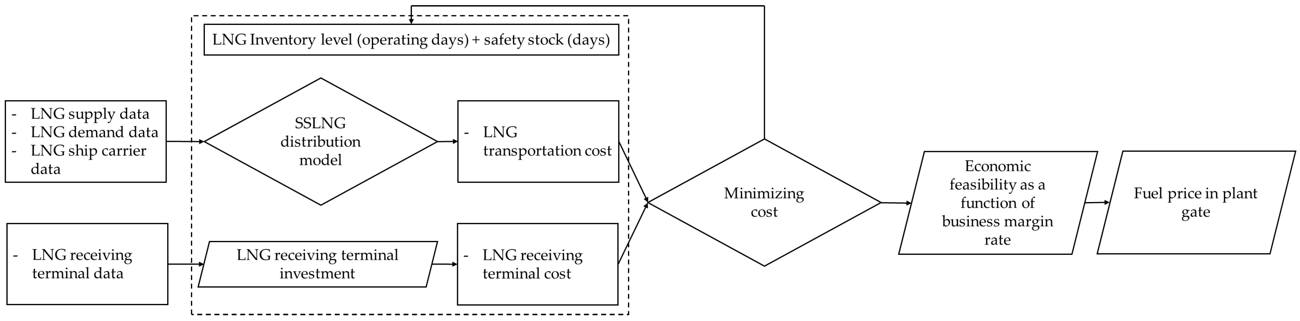
2. Methodology
2.1. System Description
2.1.1. Mathematical Model for SSLNG Distribution Cost
| Sets | |
| N | Set of all nodes or locations |
| D ⊆ N | Set of depot nodes |
| T ⊆ N | Set of terminal nodes |
| K | Set of ships |
| Indices |
| i, j | Location points (i, j = 0, 1, 2, …, N) |
| k | Ship k (k = 0, 1, 2, …, K) |
| Notation | |
| dij | Distance from point i to point j (km) |
| fk | Fuel consumption of ship k (tons per km) |
| fc | Fuel cost (USD per ton) |
| ef | Emission rate (tons of CO2 per ton of fuel) |
| ct | Carbon cost or carbon tax (USD per ton of CO2) |
| vk | Speed of ship k (km per hour) |
| ts | Stoppage time for loading/unloading (hours) |
| rk | Charter cost of ship k (USD per hour) |
| qj | Demand at point j (BBTU per day) |
| sf | Safety stock factor (days) |
| capk | Capacity of ship k (BBTU) |
| ts | LNG unloading time (hours) |
| Decision Variables | |
| xijk | Binary variable, 1 if distribution occurs from iii to j using ship k, 0 otherwise |
| yk | Binary variable, 1 if ship k is used, 0 otherwise |
| ui | Continuous variable used for sub-tour elimination (MTZ formula) |
2.1.2. Handling and Storage Cost Formulation
| Total capex terminal | = Total capital expenditure of the FSRU terminal (USD) |
| CapexFSRU | = Capital expenditure of the FSRU (USD/m3 LNG) |
| LNG storage | = Total inventory, including operating and safety stock (m3 LNG) |
| CapexJetty&Facility | = Cost of jetty, pipeline, and onshore facilities (USD/m3 LNG) |
| ICC | = The total Initial Capital Cost during the construction phase or the total Capex of the LNG terminal; |
| Con | = The construction cost; |
| Own | = The project implementation expenses covered by FSRU project stakeholders; |
| Cont | = The contingency costs for unforeseen events. |
2.1.3. Total Unit Cost Formulation
| Total unit cost | = the combined cost of transportation, storage, and regasification at the FSRU (USD/MMBTU); |
| Transportation cost | = the total transportation expense (formulated in Equation (1)) based on LNG demand or inventory (USD); |
| Total LNG trans. | = the total amount of LNG, measured in energy units, delivered from the depot to the LNG terminal (MMBTU); |
| ICC | = the total Initial Capital Cost (USD), as formulated in Equation (13); |
| Salvage value | = the residual value of the LNG terminal assets at the end of their operational lifetime (USD); |
| Project lifetime | = the operational lifespan of the LNG terminal (years); |
| Opex LNG terminal | = the operational costs of the LNG terminal (USD/year); |
| Daily LNG demand | = the amount of LNG required by the terminal (MMBTU/day). |
2.2. Economic Feasibility
| NPV | = Net Present Value (USD); |
| Ct | = Cash flow in year t (USD); |
| r | = Discount rate (%); |
| t | = Time period (years); |
| n | = Total project lifetime (years). |
| IRR | = The rate of return that equates to cash inflows and outflows; |
| Ct | = The cash flow at time t (USD); |
| t | = The time period (years); |
| n | = The total project lifetime (years). |
| PBP | = The duration (in years) needed to recoup the investment. |
| Investment | = The total capital expenditure of the project (USD). |
| Annual net cash flow | = The yearly net income generated by the investment after deducting key expense (USD/year). |
2.3. General Assumptions in SS LNG Supply Chain Modeling
3. Results and Discussion
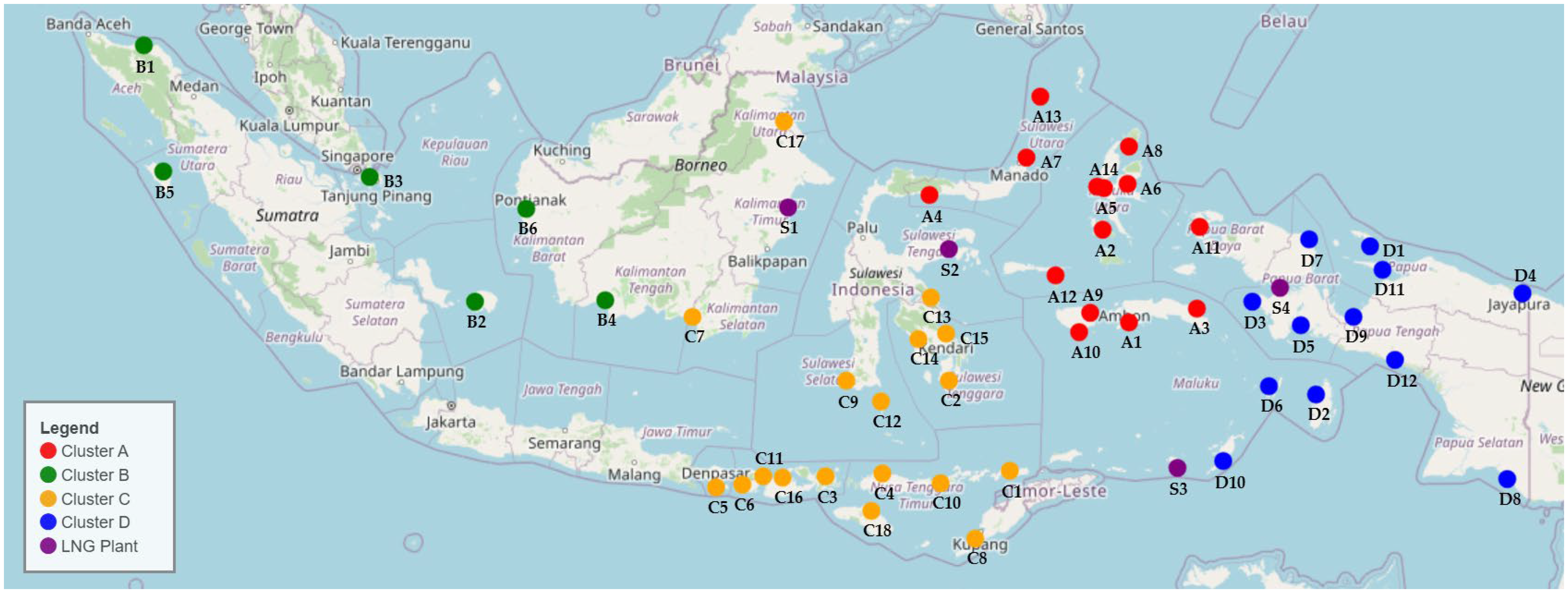
3.1. Clustering Supply and Demand
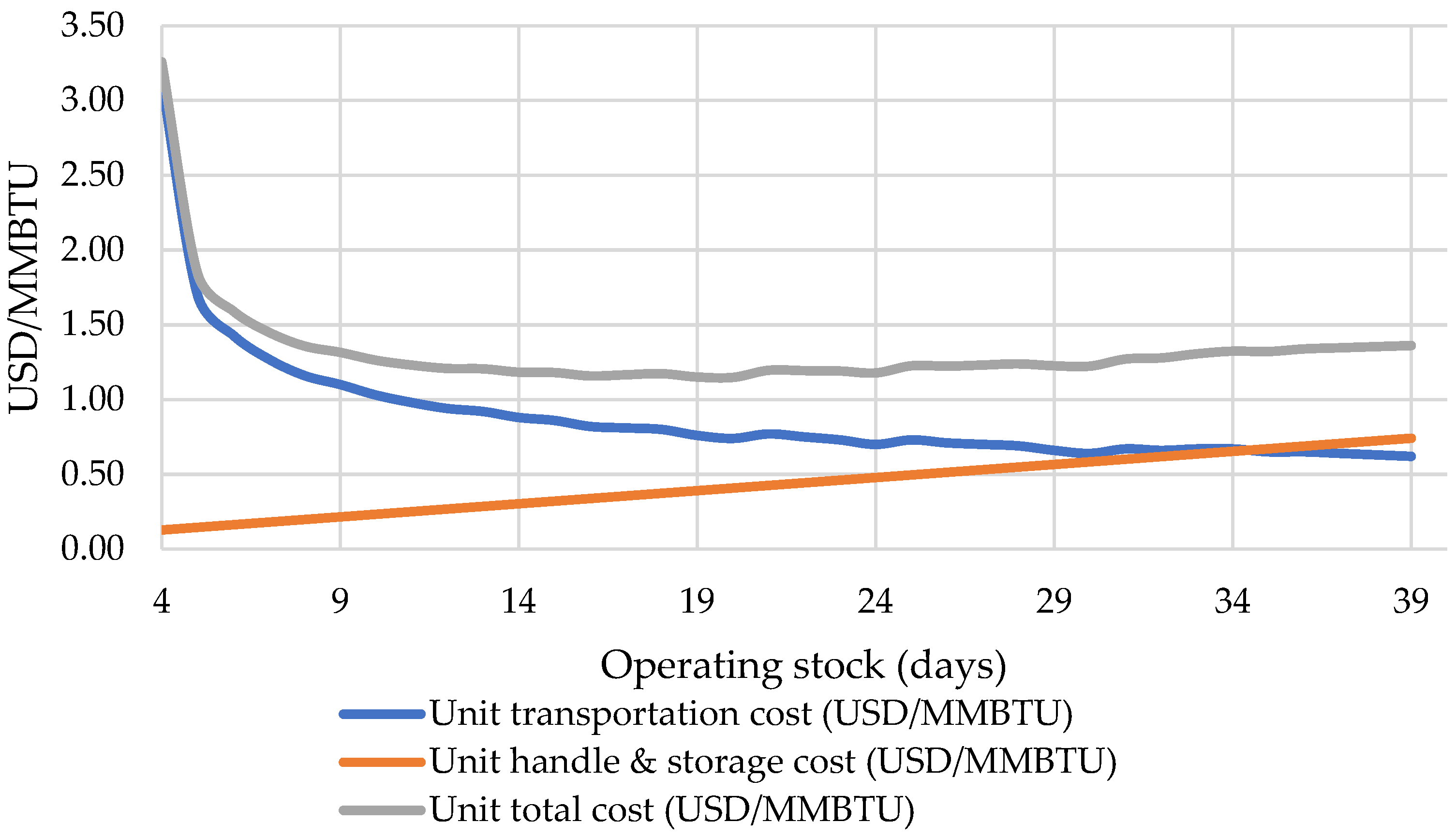
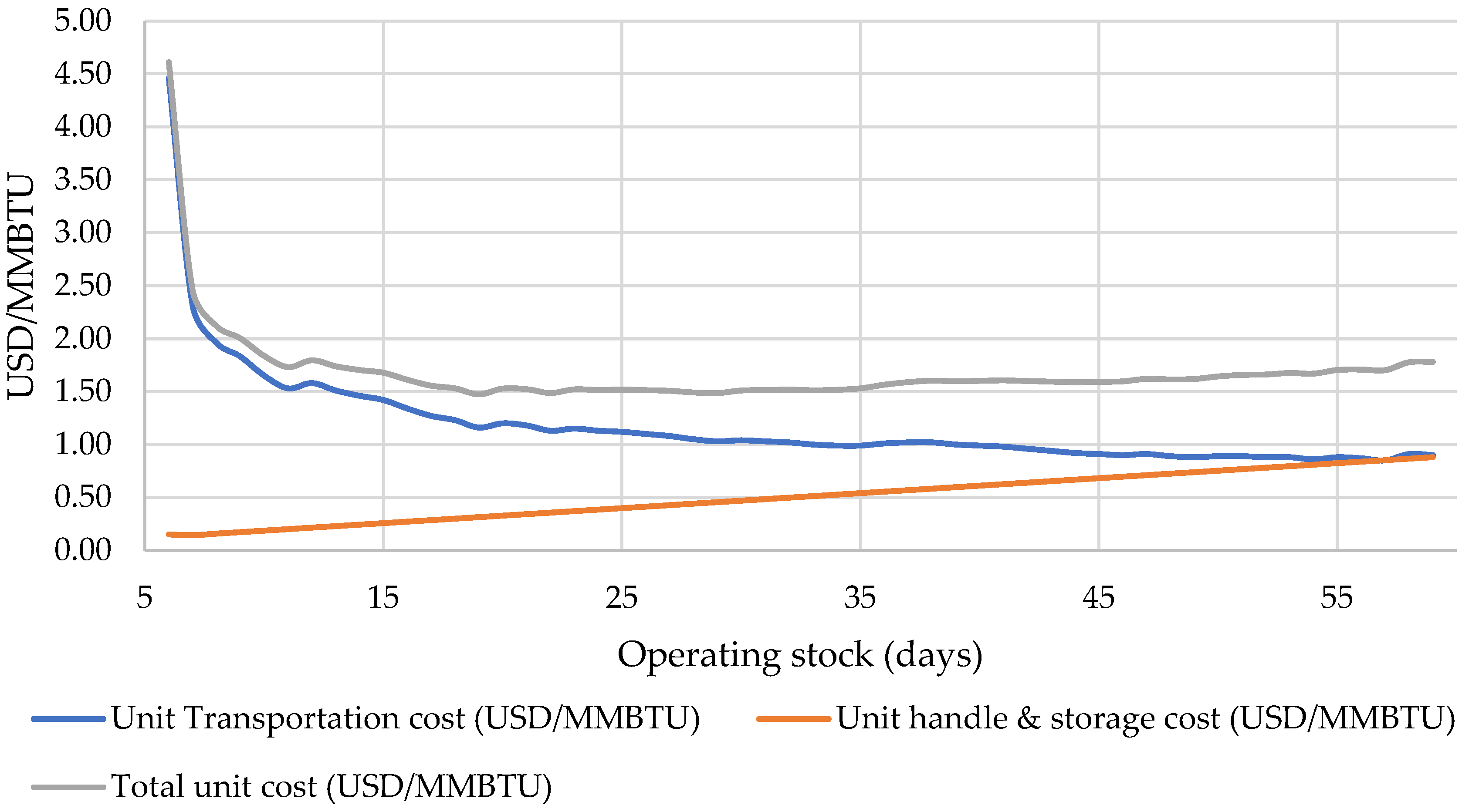
3.2. Cost Optimization and Economic Feasibility
3.2.1. Cluster A
3.2.2. Cluster B
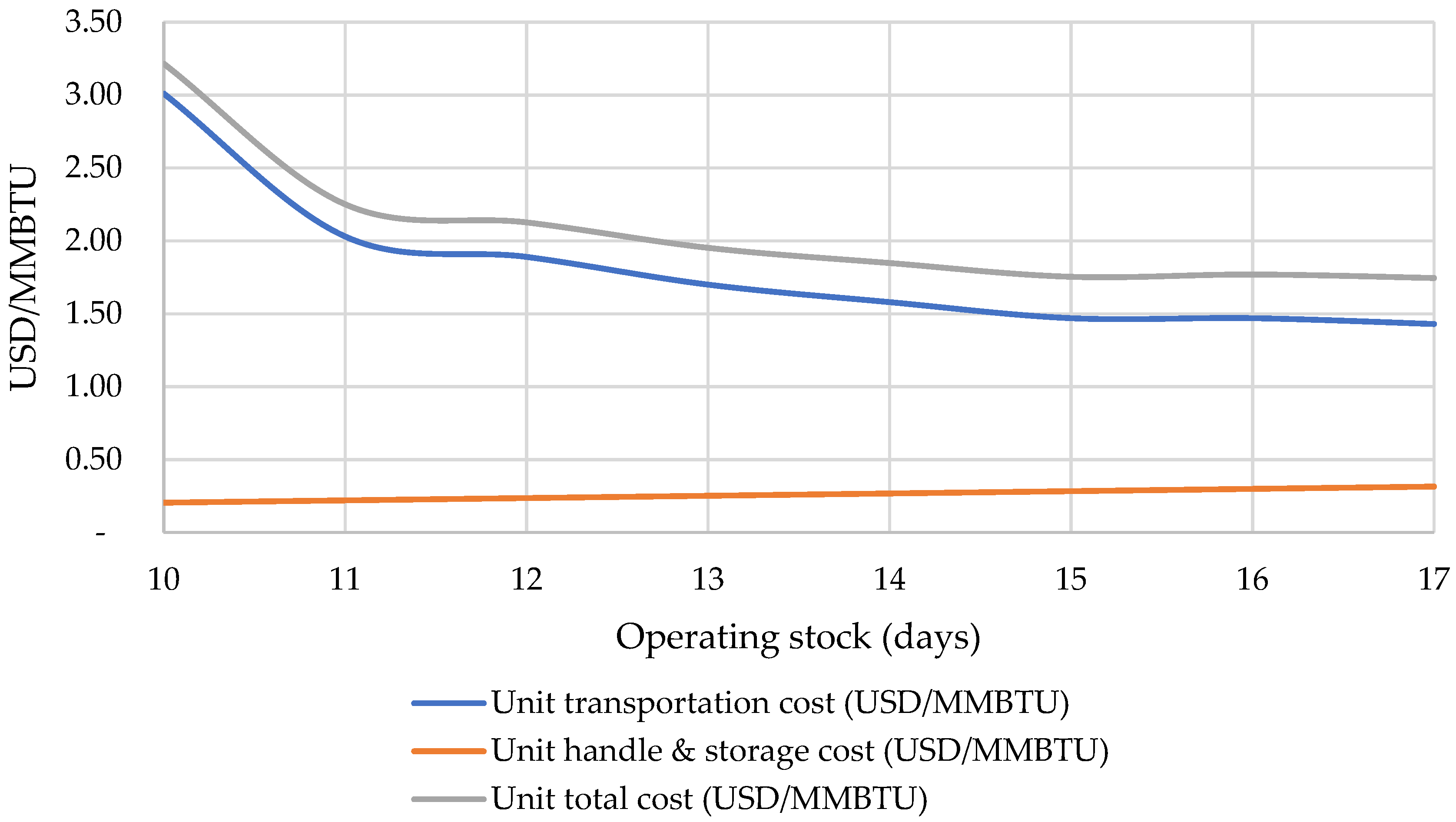
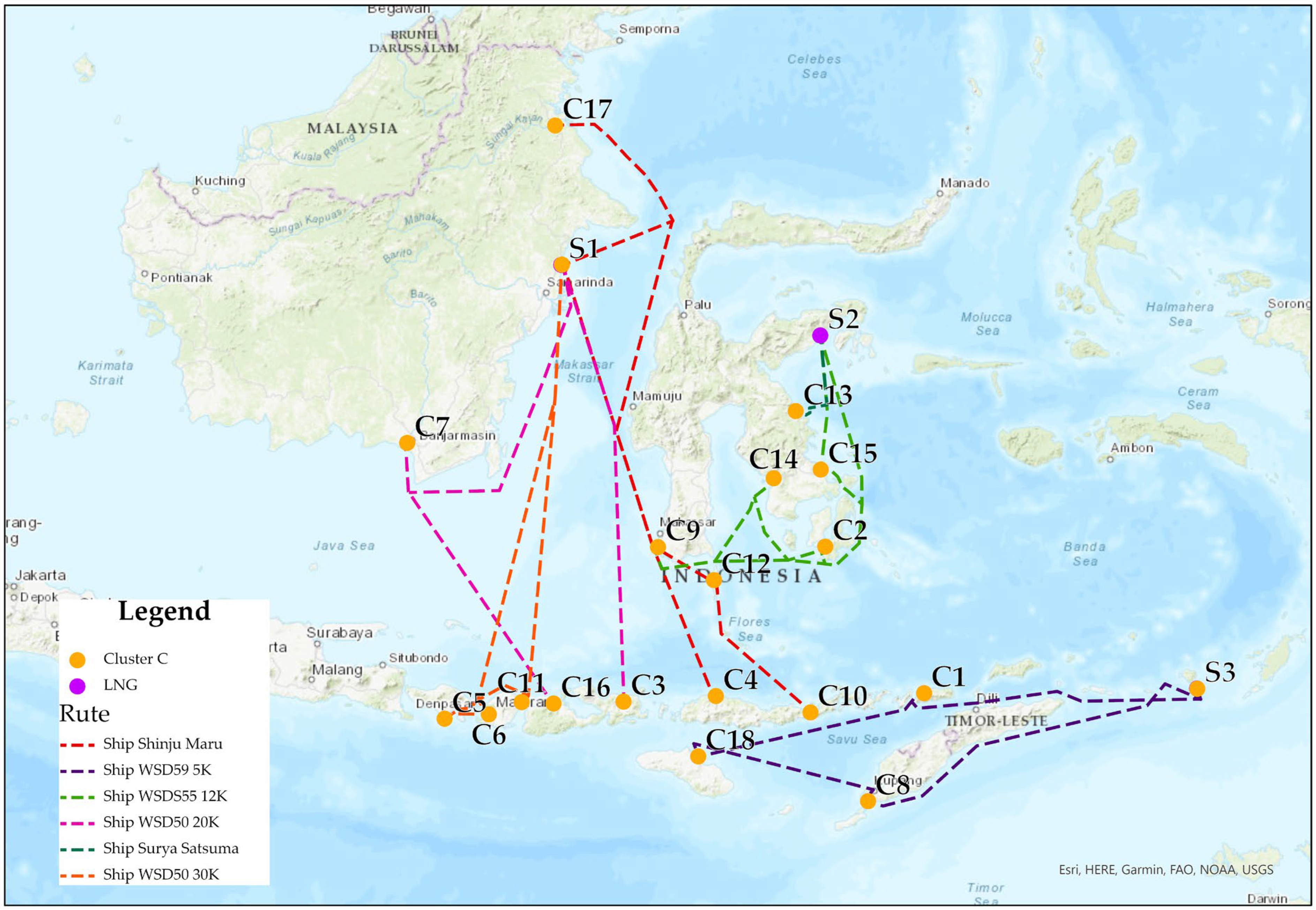
3.2.3. Cluster C
3.2.4. Cluster D
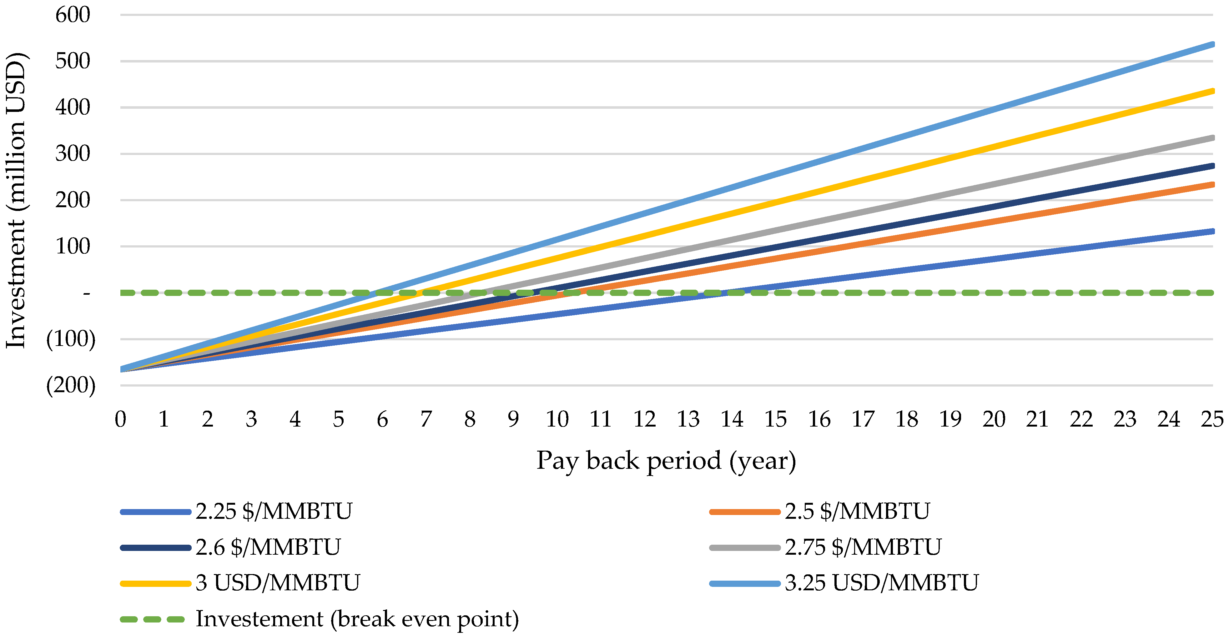
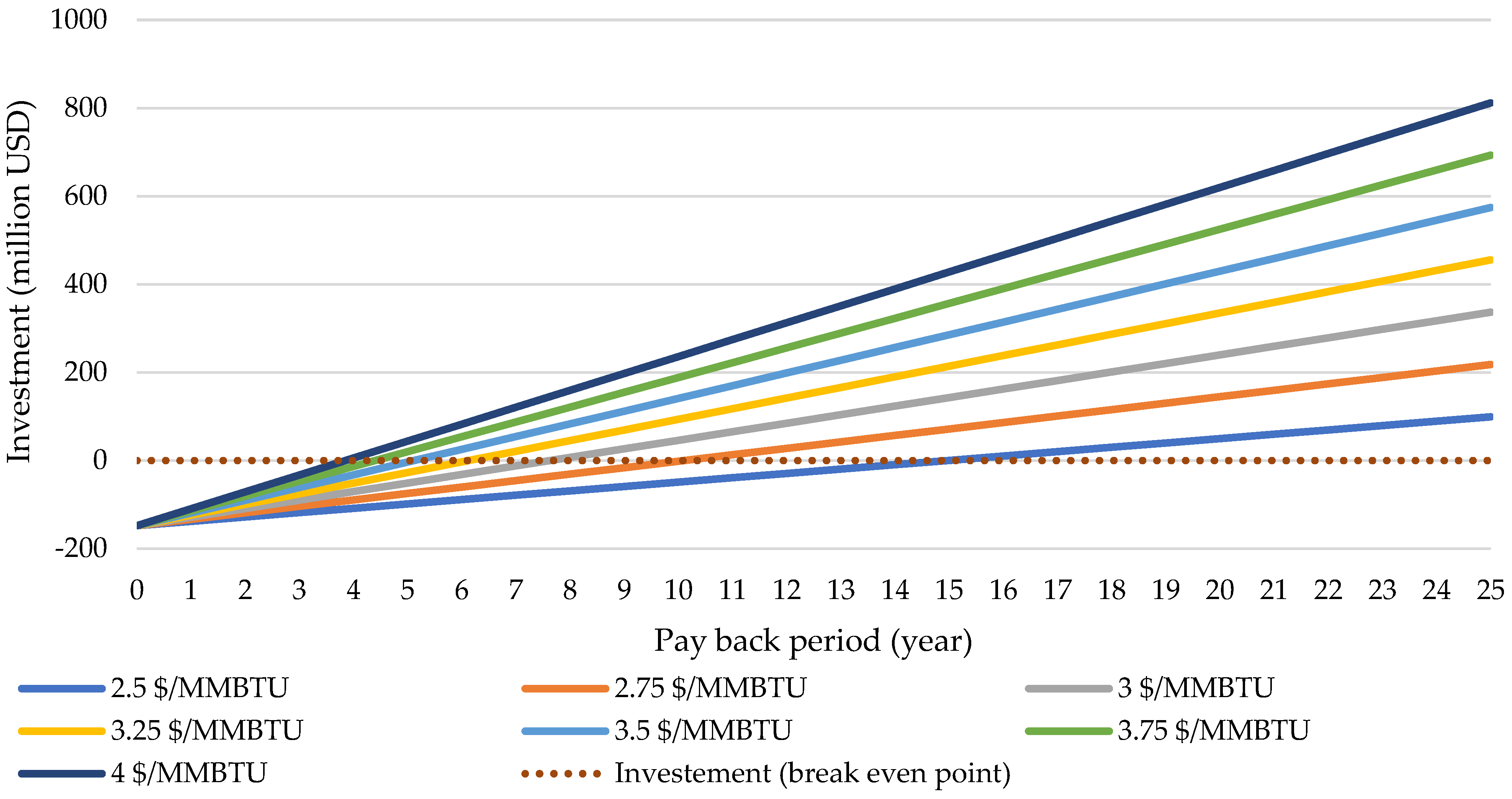
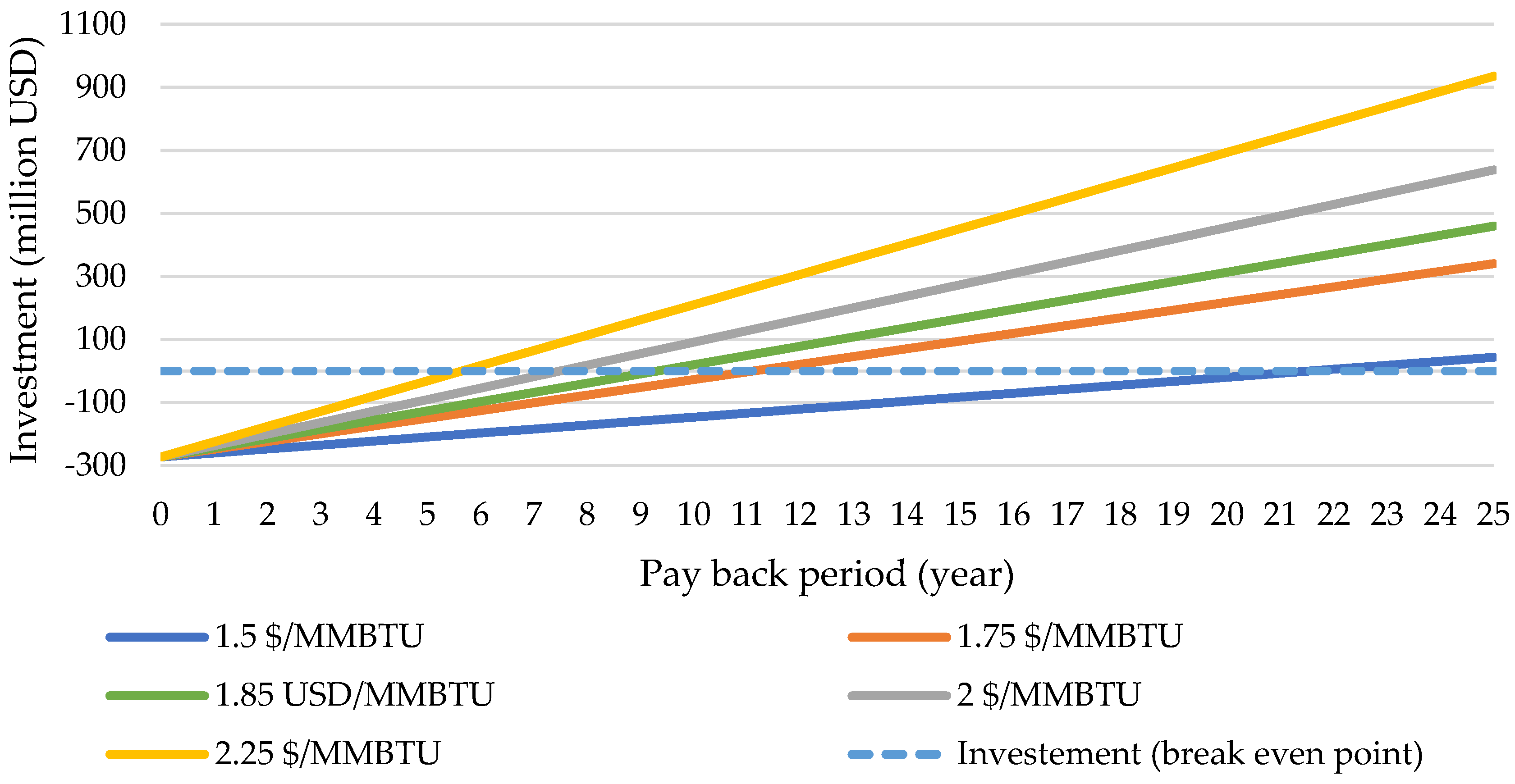
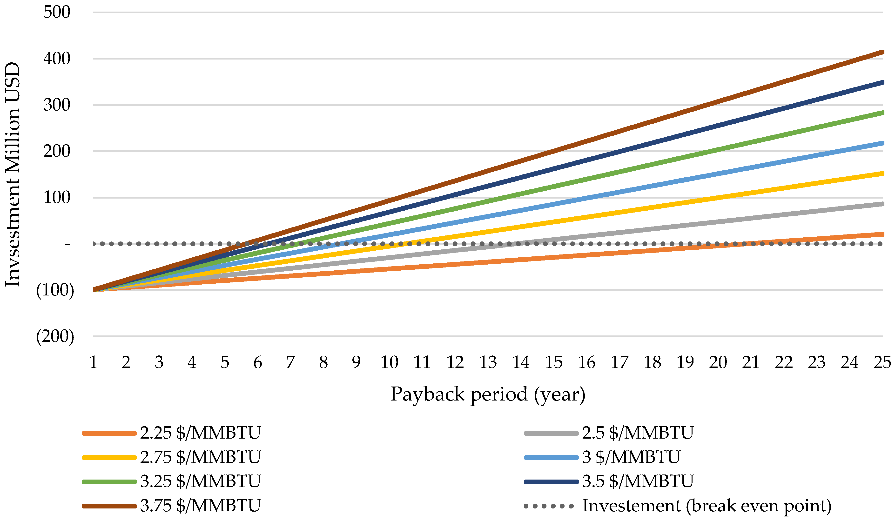
3.3. Investment Value and Fuel Costs
4. Conclusions
Author Contributions
Funding
Data Availability Statement
Conflicts of Interest
Abbreviations
| Capex | Capital expenditure |
| CVRP | Capacitated Vehicle Routing Problem |
| FSRU | Floating Storage Regasification Unit |
| HSD | High-Speed Diesel |
| ICC | Total Initial Capital Cost |
| IRR | Internal Rate of Return |
| LNG | Liquefied natural gas |
| MDCVRP | Multi-Depot Capacitated Vehicle Routing Problem |
| MILP | Mixed Integer Linear Programming |
| NPV | Net Present Value |
| Opex | Operational Expenditure |
| PBP | Time required to recover an investment |
| SS LNG | Small-scale liquefied natural gas |
Appendix A

| LNG Carrier | Capacity (m3) | Capacity (BBTU) | Speed (Knot) | Speed (km/Hour) | Fuel (Ton per km) | Rent (USD/Day) | Fuel (Ton/Day) |
|---|---|---|---|---|---|---|---|
| Shinju Maru | 2500 | 52.97 | 13 | 24.08 | 0.013331 | 11,679 | 7.7 |
| WSD59 3K | 3000 | 63.56 | 12 | 22.22 | 0.019487 | 12,730 | 10.4 |
| WSD59 5K | 5000 | 105.93 | 14 | 25.93 | 0.026533 | 16,933 | 16.5 |
| WSD59 6.5K | 6500 | 137.71 | 13 | 24.08 | 0.023547 | 20,085 | 13.6 |
| Coral Methane | 7500 | 158.90 | 14 | 25.93 | 0.032935 | 22,187 | 20.5 |
| Norgas | 10,000 | 211.86 | 14 | 25.93 | 0.042730 | 27,441 | 26.6 |
| WSDS55 12K | 12,000 | 254.24 | 14 | 25.93 | 0.030042 | 31,643 | 18.7 |
| Coral Energy | 15,600 | 330.51 | 15 | 27.78 | 0.065083 | 39,207 | 43.4 |
| WSD50 20K | 20,000 | 423.73 | 15 | 27.78 | 0.037653 | 42,538 | 25.1 |
| Surya Satsuma | 23,000 | 487.29 | 15 | 27.78 | 0.094204 | 44,808 | 62.8 |
| WSD50 30K | 30,000 | 635.59 | 16 | 29.63 | 0.048937 | 69,464 | 34.8 |
| Terminal | Cluster, Terminal Number | Latitude | Longitude | BBTUD | m3 LNG/Day | Remark |
|---|---|---|---|---|---|---|
| Ambon and Seram 1 | A1 | −3.54956 | 128.3335 | 6.51 | 307.27 | Proposed LNG terminal facility |
| Bacan | A2 | −0.63148 | 127.4862 | 0.73 | 34.46 | Proposed LNG terminal facility |
| Bula | A3 | −3.0994 | 130.4926 | 0.93 | 43.9 | Proposed LNG terminal facility |
| FSRU Gorontalo | A4 | 0.464411 | 122.0072 | 5.11 | 241.19 | Existing terminal facility |
| Halmahera, Sofifi, and Tidore 2 | A5 | 0.703122 | 127.5269 | 3.52 | 166.14 | Proposed LNG terminal facility |
| Halmahera Timur | A6 | 0.838249 | 128.2552 | 16.08 | 758.98 | Proposed LNG terminal facility |
| Minahasa | A7 | 1.679776 | 125.0795 | 10.72 | 505.98 | Proposed LNG terminal facility |
| Morotai and Tobelo 3 | A8 | 2.037213 | 128.2987 | 2.35 | 110.92 | Proposed LNG terminal facility |
| Namlea | A9 | −3.23225 | 127.1099 | 1.2 | 56.64 | Proposed LNG terminal facility |
| Namrole | A10 | −3.84501 | 126.7478 | 0.81 | 38.23 | Proposed LNG terminal facility |
| Raja Ampat | A11 | −0.53295 | 130.5775 | 0.71 | 33.51 | Proposed LNG terminal facility |
| Sanana | A12 | −2.07 | 125.9798 | 0.87 | 41.06 | Proposed LNG terminal facility |
| Tahuna | A13 | 3.615112 | 125.4952 | 2.42 | 114.22 | Proposed LNG terminal facility |
| Ternate | A14 | 0.768278 | 127.3065 | 5.65 | 266.68 | Proposed LNG terminal facility |
| Arun PAG | B1 | 5.2156 | 97.08788 | 16.2 | 764.64 | Existing terminal facility |
| Belitung | B2 | −2.8905 | 107.5653 | 2.1 | 99.12 | Proposed LNG terminal facility |
| Bintan | B3 | 1.064211 | 104.2365 | 0.7 | 33.04 | Proposed LNG terminal facility |
| Kalteng | B4 | −2.8532 | 111.6955 | 4.86 | 229.392 | Proposed LNG terminal facility |
| Nias | B5 | 1.210076 | 97.67568 | 6.6 | 311.52 | Proposed LNG terminal facility |
| Pontianak | B6 | 0.063473 | 109.2001 | 36.28 | 1712.416 | Proposed LNG terminal facility |
| Alor | C1 | −8.2479 | 124.5489 | 1.35 | 63.72 | Proposed LNG terminal facility |
| Baubau | C2 | −5.39652 | 122.6252 | 5.27 | 248.744 | Proposed LNG terminal facility |
| Bima | C3 | −8.40963 | 118.6968 | 7.35 | 346.92 | Proposed LNG terminal facility |
| Flores | C4 | −8.30431 | 120.4959 | 0.77 | 36.344 | Proposed LNG terminal facility |
| FSRU Karunia Dewata | C5 | −8.74677 | 115.2107 | 29.6 | 1397.12 | Existing terminal facility |
| Jeranjang Lombok 4 | C6 | −8.65981 | 116.0716 | 20.86 | 984.592 | Proposed LNG terminal facility |
| Kalsel | C7 | −3.37403 | 114.4828 | 10.08 | 475.776 | Proposed LNG terminal facility |
| Kupang peaker | C8 | −10.3526 | 123.459 | 2.92 | 137.824 | Proposed LNG terminal facility |
| Makassar | C9 | −5.4033 | 119.37 | 9.6 | 453.12 | Proposed LNG terminal facility |
| Maumere | C10 | −8.62013 | 122.3366 | 1.54 | 72.688 | Proposed LNG terminal facility |
| Sambelia | C11 | −8.42181 | 116.7109 | 2.6 | 122.72 | Proposed LNG terminal facility |
| Selayar | C12 | −6.04827 | 120.4582 | 1.66 | 78.352 | Proposed LNG terminal facility |
| Sulbagsel | C13 | −2.7564 | 122.053 | 42.46 | 2004.112 | Proposed LNG terminal facility |
| Sulselbar | C14 | −4.06503 | 121.6202 | 5.03 | 237.416 | Proposed LNG terminal facility |
| Sultra | C15 | −3.89476 | 122.5393 | 2.1 | 99.12 | Proposed LNG terminal facility |
| Sumbawa | C16 | −8.44733 | 117.333 | 19.75 | 932.2 | Proposed LNG terminal facility |
| Tanjung selor | C17 | 2.813909 | 117.3644 | 0.66 | 31.152 | Proposed LNG terminal facility |
| Waingapu | C18 | −9.47733 | 120.1521 | 3.48 | 164.256 | Proposed LNG terminal facility |
| Biak | D1 | −1.14437 | 135.9474 | 3.45 | 162.84 | Proposed LNG terminal facility |
| Dobo | D2 | −5.81997 | 134.2446 | 1.01 | 47.672 | Proposed LNG terminal facility |
| Fak-fak | D3 | −2.91949 | 132.2193 | 1.46 | 68.912 | Proposed LNG terminal facility |
| Jayapura | D4 | −2.61653 | 140.7867 | 7.09 | 334.648 | Proposed LNG terminal facility |
| Kaimana | D5 | −3.66659 | 133.7623 | 0.6 | 28.32 | Proposed LNG terminal facility |
| Langgur | D6 | −5.55358 | 132.7717 | 1.59 | 75.048 | Proposed LNG terminal facility |
| Manokwari | D7 | −0.93527 | 134.012 | 7.39 | 348.808 | Proposed LNG terminal facility |
| Merauke | D8 | −8.47729 | 140.3374 | 4.41 | 208.152 | Proposed LNG terminal facility |
| Nabire | D9 | −3.37871 | 135.455 | 2.3 | 108.56 | Proposed LNG terminal facility |
| Saumlaki | D10 | −7.93842 | 131.2967 | 0.83 | 39.176 | Proposed LNG terminal facility |
| Serui | D11 | −1.88209 | 136.3736 | 1.14 | 53.808 | Proposed LNG terminal facility |
| Timika | D12 | −4.75358 | 136.7653 | 7.16 | 337.952 | Proposed LNG terminal facility |
| Bontang NGL | S1 | 0.100036 | 117.4962 | 0 | 0 | Existing LNG Plant |
| Donggi Senoro | S2 | −1.24916 | 122.5889 | 0 | 0 | Existing LNG Plant |
| Masela | S3 | −8.16121 | 129.8702 | 0 | 0 | Proposed LNG Plant |
| Tangguh | S4 | −2.44209 | 133.1205 | 0 | 0 | Existing LNG Plant |
| Location | A1 | A2 | A3 | A4 | A5 | A6 | A7 | A8 | A9 | A10 | A11 | A12 | A13 | A14 | S1 | S2 | S3 | S4 | |
|---|---|---|---|---|---|---|---|---|---|---|---|---|---|---|---|---|---|---|---|
| A1 | Ambon and Seram | 442 | 414 | 886 | 674 | 717 | 747 | 824 | 159 | 206 | 660 | 340 | 939 | 594 | 1648 | 796 | 612 | 605 | |
| A2 | Bacan | 442 | 468 | 649 | 440 | 484 | 432 | 528 | 326 | 488 | 455 | 242 | 597 | 252 | 1322 | 580 | 989 | 719 | |
| A3 | Bula | 414 | 468 | 1036 | 553 | 561 | 834 | 668 | 429 | 560 | 430 | 527 | 999 | 653 | 1724 | 938 | 636 | 303 | |
| A4 | FSRU Gorontalo | 886 | 649 | 1036 | 1022 | 1002 | 472 | 805 | 770 | 758 | 1038 | 551 | 695 | 599 | 1394 | 366 | 1376 | 1295 | |
| A5 | Halmahera, Sofifi, and Tidore | 674 | 440 | 553 | 1022 | 492 | 805 | 452 | 558 | 690 | 424 | 373 | 877 | 625 | 1694 | 954 | 1222 | 904 | |
| A6 | Halmahera Timur | 717 | 484 | 561 | 1002 | 492 | 647 | 222 | 601 | 733 | 370 | 642 | 646 | 475 | 1464 | 997 | 1180 | 812 | |
| A7 | Minahasa | 747 | 432 | 834 | 472 | 805 | 647 | 450 | 630 | 711 | 821 | 503 | 321 | 295 | 1020 | 494 | 1294 | 1085 | |
| A8 | Morotai and Tobelo | 824 | 528 | 668 | 805 | 452 | 222 | 450 | 708 | 897 | 457 | 649 | 449 | 278 | 1267 | 821 | 1287 | 919 | |
| A9 | Namlea | 159 | 326 | 429 | 770 | 558 | 601 | 630 | 708 | 174 | 544 | 224 | 823 | 478 | 1532 | 653 | 706 | 699 | |
| A10 | Namrole | 206 | 488 | 560 | 758 | 690 | 733 | 711 | 897 | 174 | 675 | 284 | 926 | 620 | 1562 | 594 | 654 | 774 | |
| A11 | Raja Ampat | 660 | 455 | 430 | 1038 | 424 | 370 | 821 | 457 | 544 | 675 | 599 | 882 | 640 | 1700 | 696 | 1049 | 681 | |
| A12 | Sanana | 340 | 242 | 527 | 551 | 373 | 642 | 503 | 649 | 224 | 284 | 599 | 708 | 373 | 1407 | 443 | 887 | 796 | |
| A13 | Tahuna | 939 | 597 | 999 | 695 | 877 | 646 | 321 | 449 | 823 | 926 | 882 | 708 | 389 | 969 | 717 | 1487 | 1250 | |
| A14 | Ternate | 594 | 252 | 653 | 599 | 625 | 475 | 295 | 278 | 478 | 620 | 640 | 373 | 389 | 1155 | 589 | 1141 | 904 | |
| S1 | Bontang NGL | 1648 | 1322 | 1724 | 1394 | 1694 | 1464 | 1020 | 1267 | 1532 | 1562 | 1700 | 1407 | 969 | 1155 | 1416 | 1935 | 1975 | |
| S2 | Donggi Senoro | 796 | 580 | 938 | 366 | 954 | 997 | 494 | 821 | 653 | 594 | 696 | 443 | 717 | 589 | 1416 | 1200 | 1209 | |
| S3 | Masela | 612 | 989 | 636 | 1376 | 1222 | 1180 | 1294 | 1287 | 706 | 654 | 1049 | 887 | 1487 | 1141 | 1935 | 1200 | 816 | |
| S4 | Tangguh | 605 | 719 | 303 | 1295 | 904 | 812 | 1085 | 919 | 699 | 774 | 681 | 796 | 1250 | 904 | 1975 | 1209 | 816 |
| Location | Arun PAG | Belitung | Bintan | Kalteng | Nias | Pontianak | Bontang NGL | Donggi Senoro | Masela | Tangguh | |
|---|---|---|---|---|---|---|---|---|---|---|---|
| B1 | Arun PAG | 1588 | 969 | 2105 | 848 | 1537 | 3060 | 3844 | 4141 | 4538 | |
| B2 | Belitung | 1588 | 669 | 723 | 2203 | 411 | 1678 | 2463 | 2760 | 3157 | |
| B3 | Bintan | 969 | 669 | 1185 | 1766 | 617 | 2140 | 2924 | 3221 | 3618 | |
| B4 | Kalteng | 2105 | 723 | 1185 | 2065 | 781 | 1130 | 1922 | 2219 | 2616 | |
| B5 | Nias | 848 | 2203 | 1766 | 2065 | 2261 | 2995 | 3749 | 4022 | 4444 | |
| B6 | Pontianak | 1537 | 411 | 617 | 781 | 2261 | 1736 | 2520 | 2817 | 3214 | |
| S1 | Bontang NGL | 3060 | 1678 | 2140 | 1130 | 2995 | 1736 | 1416 | 1935 | 1975 | |
| S2 | Donggi Senoro | 3844 | 2463 | 2924 | 1922 | 3749 | 2520 | 1416 | 1200 | 1209 | |
| S3 | Masela | 4141 | 2760 | 3221 | 2219 | 4022 | 2817 | 1935 | 1200 | 816 | |
| S4 | Tangguh | 4538 | 3157 | 3618 | 2616 | 4444 | 3214 | 1975 | 1209 | 816 |
| Location | C1 | C2 | C3 | C4 | C5 | C6 | C7 | C8 | C9 | C10 | C11 | C12 | C13 | C14 | C15 | C16 | C17 | C18 | S1 | S2 | S3 | S4 | |
|---|---|---|---|---|---|---|---|---|---|---|---|---|---|---|---|---|---|---|---|---|---|---|---|
| C1 | Alor | 429 | 682 | 501 | 1065 | 1017 | 1319 | 281 | 791 | 329 | 911 | 613 | 777 | 632 | 652 | 843 | 1778 | 511 | 1360 | 888 | 702 | 1225 | |
| C2 | Baubau | 429 | 557 | 4545 | 909 | 861 | 1032 | 811 | 447 | 371 | 759 | 309 | 557 | 280 | 432 | 693 | 1474 | 1061 | 1055 | 668 | 971 | 1363 | |
| C3 | Bima | 682 | 557 | 252 | 428 | 380 | 758 | 1093 | 690 | 437 | 274 | 337 | 1012 | 594 | 887 | 206 | 1392 | 730 | 972 | 1123 | 1310 | 1766 | |
| C4 | Flores | 501 | 4545 | 252 | 635 | 586 | 913 | 912 | 608 | 256 | 481 | 263 | 863 | 505 | 738 | 413 | 1421 | 937 | 1002 | 974 | 1129 | 1585 | |
| C5 | FSRU Karunia Dewata | 1065 | 909 | 428 | 635 | 100 | 676 | 972 | 1007 | 820 | 237 | 665 | 1364 | 911 | 1239 | 277 | 1546 | 579 | 1065 | 1476 | 1677 | 2147 | |
| C6 | Jeranjang Lombok | 1017 | 861 | 380 | 586 | 100 | 627 | 950 | 958 | 772 | 195 | 617 | 1316 | 863 | 1191 | 229 | 1497 | 556 | 1017 | 1427 | 1645 | 2098 | |
| C7 | Kalsel | 1319 | 1032 | 758 | 913 | 676 | 627 | 1506 | 1114 | 1095 | 656 | 799 | 1504 | 1018 | 1379 | 670 | 755 | 1112 | 822 | 1615 | 1912 | 2309 | |
| C8 | Kupang peaker | 281 | 811 | 1093 | 912 | 972 | 950 | 1506 | 1180 | 740 | 882 | 1010 | 1148 | 1021 | 1066 | 963 | 2175 | 457 | 1757 | 1235 | 812 | 1448 | |
| C9 | Makassar | 791 | 447 | 690 | 608 | 1007 | 958 | 1114 | 1180 | 675 | 864 | 391 | 804 | 420 | 782 | 801 | 1556 | 1320 | 1138 | 1000 | 1340 | 1733 | |
| C10 | Maumere | 329 | 371 | 437 | 256 | 820 | 772 | 1095 | 740 | 675 | 666 | 402 | 767 | 535 | 642 | 598 | 1571 | 990 | 1152 | 878 | 958 | 1437 | |
| C11 | Sambelia | 911 | 759 | 274 | 481 | 237 | 195 | 656 | 882 | 864 | 666 | 517 | 1213 | 768 | 1088 | 114 | 1454 | 489 | 996 | 1325 | 1539 | 1992 | |
| C12 | Selayar | 613 | 309 | 337 | 263 | 665 | 617 | 799 | 1010 | 391 | 402 | 517 | 780 | 295 | 655 | 454 | 1242 | 973 | 824 | 892 | 1188 | 1586 | |
| C13 | Sulbagsel | 777 | 557 | 1012 | 863 | 1364 | 1316 | 1504 | 1148 | 804 | 767 | 1213 | 780 | 663 | 114 | 1148 | 1556 | 1398 | 1527 | 325 | 1117 | 1231 | |
| C14 | Sulselbar | 632 | 280 | 594 | 505 | 911 | 863 | 1018 | 1021 | 420 | 535 | 768 | 295 | 663 | 641 | 705 | 1461 | 1224 | 1042 | 860 | 1181 | 1574 | |
| C15 | Sultra | 652 | 432 | 887 | 738 | 1239 | 1191 | 1379 | 1066 | 782 | 642 | 1088 | 655 | 114 | 641 | 1023 | 1620 | 1316 | 1402 | 296 | 1038 | 1225 | |
| C16 | Sumbawa | 843 | 693 | 206 | 413 | 277 | 229 | 670 | 963 | 801 | 598 | 114 | 454 | 1148 | 705 | 1023 | 1436 | 570 | 982 | 1260 | 1471 | 1924 | |
| C17 | Tanjung selor | 1778 | 1474 | 1392 | 1421 | 1546 | 1497 | 755 | 2175 | 1556 | 1571 | 1454 | 1242 | 1556 | 1461 | 1620 | 1436 | 1910 | 588 | 1403 | 2183 | 1962 | |
| C18 | Waingapu | 511 | 1061 | 730 | 937 | 579 | 556 | 1112 | 457 | 1320 | 990 | 489 | 973 | 1398 | 1224 | 1316 | 570 | 1910 | 1452 | 1485 | 1123 | 1698 | |
| S1 | Bontang NGL | 1360 | 1055 | 972 | 1002 | 1065 | 1017 | 822 | 1757 | 1138 | 1152 | 996 | 824 | 1527 | 1042 | 1402 | 982 | 588 | 1452 | 1416 | 1935 | 1975 | |
| S2 | Donggi Senoro | 888 | 668 | 1123 | 974 | 1476 | 1427 | 1615 | 1235 | 1000 | 878 | 1325 | 892 | 325 | 860 | 296 | 1260 | 1403 | 1485 | 1416 | 1200 | 1209 | |
| S3 | Masela | 702 | 971 | 1310 | 1129 | 1677 | 1645 | 1912 | 812 | 1340 | 958 | 1539 | 1188 | 1117 | 1181 | 1038 | 1471 | 2183 | 1123 | 1935 | 1200 | 816 | |
| S4 | Tangguh | 1225 | 1363 | 1766 | 1585 | 2147 | 2098 | 2309 | 1448 | 1733 | 1437 | 1992 | 1586 | 1231 | 1574 | 1225 | 1924 | 1962 | 1698 | 1975 | 1209 | 816 |
| D1 | D2 | D3 | D4 | D5 | D6 | D7 | D8 | D9 | D10 | D11 | D12 | S1 | S2 | S3 | S4 | ||
|---|---|---|---|---|---|---|---|---|---|---|---|---|---|---|---|---|---|
| D1 | Biak | 1508 | 1171 | 573 | 1495 | 1432 | 228 | 2323 | 1750 | 1686 | 207 | 1728 | 2173 | 1544 | 1621 | 1253 | |
| D2 | Dobo | 1508 | 410 | 2073 | 249 | 269 | 1351 | 933 | 399 | 447 | 1601 | 377 | 2230 | 1444 | 599 | 583 | |
| D3 | Fak-fak | 1171 | 410 | 1736 | 353 | 328 | 1014 | 1217 | 1294 | 652 | 1264 | 612 | 1893 | 1113 | 658 | 213 | |
| D4 | Jayapura | 573 | 2073 | 1736 | 2024 | 1997 | 791 | 2888 | 715 | 2251 | 528 | 2283 | 2734 | 2108 | 2186 | 1817 | |
| D5 | Kaimana | 1495 | 249 | 353 | 2024 | 298 | 1302 | 998 | 1583 | 597 | 1552 | 371 | 2182 | 1397 | 673 | 526 | |
| D6 | Langgur | 1432 | 269 | 328 | 1997 | 298 | 1275 | 1103 | 568 | 408 | 1525 | 546 | 2154 | 1293 | 462 | 494 | |
| D7 | Manokwari | 228 | 1351 | 1014 | 791 | 1302 | 1275 | 2166 | 334 | 1529 | 301 | 1562 | 2017 | 1386 | 1464 | 1095 | |
| D8 | Merauke | 2323 | 933 | 1217 | 2888 | 998 | 1103 | 2166 | 2447 | 1018 | 2416 | 657 | 3046 | 2197 | 1157 | 1390 | |
| D9 | Nabire | 1750 | 399 | 1294 | 715 | 1583 | 568 | 334 | 2447 | 806 | 1834 | 1842 | 2472 | 1687 | 958 | 817 | |
| D10 | Saumlaki | 1686 | 447 | 652 | 2251 | 597 | 408 | 1529 | 1018 | 806 | 1778 | 784 | 2082 | 1347 | 193 | 810 | |
| D11 | Serui | 207 | 1601 | 1264 | 528 | 1552 | 1525 | 301 | 2416 | 1834 | 1778 | 1821 | 2267 | 1636 | 1714 | 1345 | |
| D12 | Timika | 1728 | 377 | 612 | 2283 | 371 | 546 | 1562 | 657 | 1842 | 784 | 1821 | 2450 | 1666 | 936 | 795 | |
| S1 | Bontang NGL | 2173 | 2230 | 1893 | 2734 | 2182 | 2154 | 2017 | 3046 | 2472 | 2082 | 2267 | 2450 | 1416 | 1935 | 1975 | |
| S2 | Donggi Senoro | 1544 | 1444 | 1113 | 2108 | 1397 | 1293 | 1386 | 2197 | 1687 | 1347 | 1636 | 1666 | 1416 | 1200 | 1209 | |
| S3 | Masela | 1621 | 599 | 658 | 2186 | 673 | 462 | 1464 | 1157 | 958 | 193 | 1714 | 936 | 1935 | 1200 | 816 | |
| S4 | Tangguh | 1253 | 583 | 213 | 1817 | 526 | 494 | 1095 | 1390 | 817 | 810 | 1345 | 795 | 1975 | 1209 | 816 |
References
- Kementerian Energi dan Sumber Daya Mineral Republik Indonesia. Total Electricity Generation Capacity in Indonesia from 2014 to 2022 with Target for 2023; Kementerian Energi dan Sumber Daya Mineral Republik Indonesia: Jakarta, Indonesia, 2023. (In Gigawatts)
- PT. PLN (Persero). Statistik PLN 2022; PT. PLN (Persero): Jakarta, Indonesia, 2023; Available online: https://web.pln.co.id/stakeholder/laporan-statistik (accessed on 13 April 2025).
- IEA Indonesia Electricity. Available online: https://www.iea.org/countries/indonesia/electricity (accessed on 9 April 2025).
- PT. PLN (Persero). Statistik PLN 2021; PT. PLN (Persero): Jakarta, Indonesia, 2022; Available online: https://web.pln.co.id/stakeholder/laporan-statistik (accessed on 13 April 2025).
- Kementerian Energi & Sumber Daya Mineral. Rencana Usaha Penyediaan Tenaga Listrik (RUPTL) PT. PLN (Persero) 2021–2030; Kementerian Energi & Sumber Daya Mineral: Jakarta, Indonesia, 2021.
- Faramawy, S.; Zaki, T.; Sakr, A.A. Natural Gas Origin, Composition, and Processing: A Review. J. Nat. Gas Sci. Eng. 2016, 34, 34–54. [Google Scholar] [CrossRef]
- Mokhatab, S.; Poe, W.A.; Mak, J.Y. Handbook of Natural Gas Transmission and Processing; Gulf Professional Publishing: Houston, TX, USA, 2012; ISBN 9780123869142. [Google Scholar]
- Morosuk, T.; Tsatsaronis, G. LNG—Based Cogeneration Systems: Evaluation Using Exergy-Based Analyses. In Natural Gas-Extraction to End Use; InTech: Milton, QLD, USA, 2011; p. 235. [Google Scholar]
- Mokhatab, S.; Mak, J.Y.; Valappil, J.V.; Wood, D.A. LNG Fundamentals; Elsevier Inc.: Oxford, UK, 2014; ISBN 9780124045859. [Google Scholar]
- Wyllie, M. Developments in the ‘LNG to Power’ Market and the Growing Importance of Floating Facilities; OIES: Oxford, UK, 2021. [Google Scholar]
- Direktorat Jenderal Minyak dan Gas Bumi Kementerian Energi dan Sumber Daya Mineral. Satistik Minyak Dan Gas Bumi 2022; Kementerian Energi dan Sumber Daya Mineral Republik Indonesia: Jakarta, Indonesia, 2022; Available online: https://migas.esdm.go.id/cms/uploads/uploads/C--ESDM--Statistik-Tahun-2022.pdf (accessed on 13 April 2025).
- Asia-Pasific Economic Corporation. Small-Scale LNG in Asia-Pacific; Asia-Pasific Economic Corporation: Singapore, 2019. [Google Scholar]
- International Gas Union. Small Scale LNG; International Gas Union: London, UK, 2015. [Google Scholar]
- Songhurst, B. The Outlook for Floating Storage and Regasification Units (FSRUs); The Oxford Institute for Energy Studies: Oxford, UK, 2017. [Google Scholar]
- Songhurst, B. Floating Liquefaction (FLNG): Potential for Wider Deployment; The Oxford Institute for Energy Studies: Oxford, UK, 2016. [Google Scholar]
- Lim, H.; Lee, G.M.; Singgih, I.K. Multi-Depot Split-Delivery Vehicle Routing Problem. IEEE Access 2021, 9, 112206–112220. [Google Scholar] [CrossRef]
- Kim, G.; Ong, Y.S.; Heng, C.K.; Tan, P.S.; Zhang, N.A. City Vehicle Routing Problem (City VRP): A Review. IEEE Trans. Intell. Transp. Syst. 2015, 16, 1654–1666. [Google Scholar] [CrossRef]
- Braekers, K.; Ramaekers, K.; Van Nieuwenhuyse, I. The Vehicle Routing Problem: State of the Art Classification and Review. Comput. Ind. Eng. 2016, 99, 300–313. [Google Scholar] [CrossRef]
- Jokinen, R.; Pettersson, F.; Saxén, H. An MILP Model for Optimization of a Small-Scale LNG Supply Chain along a Coastline. Appl. Energy 2015, 138, 423–431. [Google Scholar] [CrossRef]
- Bittante, A.; Jokinen, R.; Krooks, J.; Pettersson, F.; Saxen, H. Optimal Design of a Small-Scale LNG Supply Chain Combining Sea and Land Transports. Ind. Eng. Chem. Res. 2017, 56, 13434–13443. [Google Scholar] [CrossRef]
- Bittante, A.; Pettersson, F.; Sax, H.; Pettersson, F.; Chain, S.; Sax, H. Optimization of a Small-Scale LNG Supply Chain. Energy 2018, 148, 79–89. [Google Scholar] [CrossRef]
- Bittante, A.; Saxén, H.; Bittante, A.; Saxén, H. Design of Small LNG Supply Chain by Multi-Period Optimization. Energies 2020, 13, 6704. [Google Scholar] [CrossRef]
- Pratiwi, E.; Handani, D.W.G.B.D.S.A.; Dinariyana, A.A.B.; Abdillah, H.N. Economic Analysis on the LNG Distribution to Power Plants in Bali and Lombok by Utilizing Mini-LNG Carriers. In Proceedings of the 5th International Conference on Marine Technology (SENTA 2020), Surabaya, Indonesia, 8 December 2020. [Google Scholar]
- Surury, F.; Syauqi, A.; Wahyu, W. Multi-Objective Optimization of Petroleum Product Logistics in Eastern Indonesia Region. Asian J. Shipp. Logist. 2021, 37, 220–230. [Google Scholar] [CrossRef]
- Budiyanto, M.A.; Putra, G.L.; Riadi, A.; Gunawan; Febri, A.M.; Theotokatos, G. Techno-economic Analysis of Natural Gas Distribution Using a Small-scale Liquefied Natural Gas Carrier. Sci. Rep. 2023, 13, 22900. [Google Scholar] [CrossRef] [PubMed]
- Budiyanto, M.A.; Pamitran, A.S.; Yusman, T. Optimization of the Route of Distribution of LNG Using Small Scale LNG Carrier: A Case Study of a Gas Power Plant in the Sumatra Region, Indonesia. Int. J. Energy Econ. Policy 2019, 9, 179–187. [Google Scholar] [CrossRef]
- Cahyo, A.; Tri, P.; Al Hakim, B.; Cahyo, A.; Tri, P.; Al Hakim, B.; Hendrik, D.; Sasmito, C.; Muttaqie, T.; Tjolleng, A.; et al. Mission Analysis of Small-Scale LNG Carrier as Feeder for East Indonesia: Ambon City as the Hub Terminal Mission Analysis of Small-Scale LNG Carrier as Feeder for East Indonesia: Ambon City as the Hub Terminal. Evergreen 2023, 10, 1938–1950. [Google Scholar]
- Budiyanto, M.A.; Riadi, A.; Buana, I.S.; Kurnia, G. Study on the LNG Distribution to Mobile Power Plants Utilizing Small-Scale LNG Carriers. Heliyon 2020, 6, e04538. [Google Scholar] [CrossRef]
- Armyn, R.; Muslim, F.; Priatna, W. Optimization of the Risk-Based Small-Scale LNG Supply Chain in the Indonesian Archipelago. Heliyon 2023, 9, e19047. [Google Scholar] [CrossRef]
- Kementerian Energi dan Sumber Daya Mineral Republik Indonesia. Keputusan Menteri Energi Dan Sumber Daya Mineral Republik Indonesia Nomor 13K/13/MEM/2020; Kementerian Energi dan Sumber Daya Mineral Republik Indonesia: Jakarta, Indonesia, 2020.
- Kementerian Energi dan Sumber Daya Mineral Republik Indonesia. Keputusan Menteri Energi Dan Sumber Daya Mineral No. 34K/16/MEM/2020; Kementerian Energi dan Sumber Daya Mineral Republik Indonesia: Jakarta, Indonesia, 2020; Volume 2020, pp. 1–22.
- Kementerian Energi dan Sumber Daya Mineral. Laporan Kinerja Direktorat Jenderal Minyak Dan Gas Bumi Kementerian Energi Dan Sumber Daya Mineral Tahun 2022; Kementerian Energi dan Sumber Daya Mineral: Jakarta, Indonesia, 2023.
- Kementerian Energi dan Sumber Daya Mineral Republik Indonesia. Direktorat Jenderal Minyak Dan Gas Bumi, Laporan Kinerja 2023; Kementerian Energi dan Sumber Daya Mineral: Jakarta, Indonesia, 2023.
- Sinaga, K.P.; Yang, M. Unsupervised K-Means Clustering Algorithm. IEEE Access 2020, 8, 80716–80727. [Google Scholar] [CrossRef]
- Li, Y.; Wu, H. A Clustering Method Based on K-Means Algorithm. In Proceedings of the 2012 International Conference on Solid State Devices and Materials Science A Clustering Method, Kyoto, Japan, 25–27 September 2012; Elsevier Srl: Amsterdam, The Netherlands, 2012; Volume 25, pp. 1104–1109. [Google Scholar]
- Shutaywi, M.; Kachouie, N.N. Silhouette Analysis for Performance Evaluation in Machine. Entropy 2021, 23, 759. [Google Scholar] [CrossRef]
- Wang, L.; Wei, L. Clustering Analysis of Dangerous Goods Transportation of Logistics Platform Based on Improved K-Means Algorithm. In Proceedings of the 2016 13th International Conference on Service Systems and Service Management (ICSSSM), Kunming, China, 24–26 June 2016; pp. 1–6. [Google Scholar]
- Blackwell, B.; Skaar, H. GOLAR LNG: Delivering the World’s First FSRUs; 2009; Volume 6. Available online: http://members.igu.org/html/wgc2009/papers/docs/wgcFinal00775.pdf (accessed on 13 April 2025).
- Lawler, E.L.; Lenstra, J.K.; Kan, A.H.G.R.; Shmoys, D. The Traveling Salesman Problem; John Wiley & Sons: Hoboken, NJ, USA, 1988; Volume 18. [Google Scholar]
- Bektas, T.; Gouveia, L. Requiem for the Miller–Tucker–Zemlin Subtour Elimination Constraints? Eur. J. Oper. Res. 2013, 236, 820–832. [Google Scholar] [CrossRef]
- Konstantinou, D.F. Developing a Life Cycle Cost Analysis Tool for Floating Storage Regasification Unit (FSRU) Operations. Diploma Thesis, National Technical University of Athens, Athens, Greece, 2020. [Google Scholar]
- Dimitriou, D.; Zeimpekis, P. Appraisal Modeling for FSRU Greenfield Energy Projects. Energies 2022, 15, 3188. [Google Scholar] [CrossRef]
- Khoiriyah, L.; Artana, K.B.; Dinariyana, A.A.B. Conceptual Design of Floating Storage and Regasification Unit (FSRU) for Eastern Part Indonesia Conceptual Design of Floating Storage and Regasification Unit (FSRU) for Eastern Part Indonesia. In Proceedings of the IOP Conference Series: Earth and Environmental Science PAPER, Kitakyushu, Japan, 2–3 June 2023. [Google Scholar]
- Jun, P.; Michael Gillenwater, W.B. CO2, CH4, and N2O Emissions from Waterborne Transportation Navigation. 2000. Available online: https://www.ipcc-nggip.iges.or.jp/public/gp/bgp/2_4_Water-borne_Navigation.pdf (accessed on 13 April 2025).
- President of Republic Indonesia. Peraturan Presiden Republik Indonesia Nomor 98 Tahun 2021; President of Republic Indonesia: Jakarta, Indonesia, 2021. [Google Scholar]
- Wartsila Developer’s Guide to Small Scale LNG Terminals. Available online: https://www.bi.go.id/id/statistik/indikator/BI-Rate.aspx (accessed on 10 January 2025).
- Eriksen, U.; Kristiansen, J.; Fagerholt, K.; Pantuso, G. Planning a Maritime Supply Chain for Liquefied Natural Gas under Uncertainty. Marit. Transp. Res. 2022, 3, 100061. [Google Scholar] [CrossRef]
- Tarlowski, J.; Sheffield, J. LNG Import Terminals-Recent Developments; MW Kellogg Ltd.: London, UK, 2012. [Google Scholar]
- Tjandranegara, A.Q.; Arsegianto, A.; Purwanto, W.W. Natural Gas as Petroleum Fuel Substitution: Analysis of Supply-Demand Projections, Infrastructures, Investments and End-User Prices. Makara J. Technol. 2011, 15, 8. [Google Scholar] [CrossRef]
- Republic of Indonesia. Undang Undang Republik Indonesia Nomor 7 Tahun 2021 Tentang Harmonisasi Peraturan Perpajakan; Republic of Indonesia: Jakarta, Indonesia, 2021. [Google Scholar]
- USAID. Global LNG Fundamentals; USAID: Washington, DC, USA, 2020.
- Ministry of Finance Indonesia. Addressing Infrastructure Financing Gap in Indonesia: Role of Financial Sector; Ministry of Finance Indonesia: Jakarta, Indonesia, 2017.
- Trading Economics Indonesia Interest Rate. Available online: https://tradingeconomics.com/indonesia/interest-rate (accessed on 4 September 2023).
- Bank of Indonesia BI 7-Day (Reverse) Repo Rate. Available online: https://www.bi.go.id/id/statistik/indikator/BI-Rate.aspx (accessed on 4 September 2023).
- Netpas Netpas Distance. Available online: https://www.netpas.net/products/detail/nd (accessed on 14 January 2025).
- Kementerian Energi dan Sumber Daya Mineral Republik Indonesia. Keputusan Menteri Energi Dan Sumber Daya Mineral Republik Indonesia No. 169.K/HK.02/MEM.M/2021; Kementerian Energi dan Sumber Daya Mineral Republik Indonesia: Jakarta, Indonesia, 2021.
- PT Indonesia Power. Laporan Statistik 2022; PT Indonesia Power: Jakarta, Indonesia, 2023. [Google Scholar]


| Item | Unit | Value/Remark | Ref. |
|---|---|---|---|
| Demand size | m3 LNG/day | Based on ref. | [5,30,31] |
| Safety stock | days | 3 | [43] |
| Operating stock | days | Varied | Assumption |
| Shipping size | m3 LNG | Daily LNG demand x Operating stock | Simulated |
| Ship fuel (HSD B35) price | USD/ton | 1163 | Assumption |
| Direct emission factor of ship engine | g CO2/kg fuel | 3.140 | [44] |
| Carbon tax | USD/t CO2 | 2 | Adapted from: [45] |
| LNG storage capacity | m3 LNG | Daily Demand x operating stock + Daily demand x safety stock | [46,47] |
| Unloading capacity | m3 LNG/hours | 10,000 | [48] |
| Unloading duration | hours | 4 | Assumption |
| Pipeline capex (including 2 compressors) | USD/km | 40,000 | [49] |
| Capex FSRU | USD/m3 LNG storage capacity | 1748.23 | [41] |
| Capex jetty, pipeline, and on shore facility | USD/m3 LNG storage capacity | 611 | [14] |
| Owner cost | % from capex terminal | 15 | [14] |
| Contingency cost | % from capex terminal | 10 | [14] |
| Sales tax | % from sales | 12 | [50] |
| Corporate tax | % earning | 22 | [50] |
| Opex | % capex terminal | 2.5 | [41] |
| Salvage value | % capex terminal | 25 | [42] |
| Depreciation | straight method for 25 years | Assumption | |
| Project lifetime | years | 25 | [42,51] |
| Equity | % total investment cost | 30 | [52] |
| Debt | % total investment cost | 70 | [52] |
| Interest rate | % | 10 | [53,54] |
| LNG Carrier Ship | Shipping Route | Demand (m3 LNG/Day) | Total Demand (m3 LNG) | Shipping Time (Days) |
|---|---|---|---|---|
| Shinju Maru | Donggi Senoro (S2) ⟶ Tahuna (A13) ⟶ Donggi Senoro (S2) | 114.22 | 2284.48 | 3.15 |
| WSD59 3K | Donggi Senoro (S2) ⟶ Namrole (A10) -> Namlea (A9) ⟶ Sanana (A12) ⟶ Donggi Senoro (S2) | 135.94 | 2718.72 | 4.02 |
| WSD59 5K | Tangguh (S4) ⟶ Raja Ampat (A11) ⟶ Halmahera, Sofifi, and Tidore (A5) ⟶ Bula (A3) -> Tangguh (S4) | 243.55 | 4871.04 | 4.48 |
| WSD59 6.5K | Donggi Senoro (S2) ⟶ Bacan (A2) ⟶ Ternate (A14) ⟶ Donggi Senoro (S2) | 301.14 | 6022.72 | 3.46 |
| Coral Methane | Donggi Senoro (S2) ⟶ FSRU Gorontalo (A4) ⟶ Donggi Senoro (S2) | 241.19 | 4823.84 | 1.84 |
| Norgas | Tangguh (S4) ⟶ Ambon and Seram (A1) ⟶ Tangguh (S4) | 486.16 | 9723.20 | 2.61 |
| WSDS55 12K | Donggi Senoro (S2) ⟶ Minahasa (A7) ⟶ Donggi Senoro (S2) | 505.98 | 10,119.68 | 2.25 |
| WSD50 20K | Tangguh (S4) ⟶ Halmahera Timur (A6) ⟶ Morotai and Tobelo (A8) ⟶ Tangguh (S4) | 981.29 | 19,625.76 | 3.93 |
| Total | 3009.47 | 60,189.44 | - |
| LNG Carrier Ship | Shipping Route | Demand (m3 LNG/Day) | Total Demand (m3 LNG) | Shipping Time (Days) |
|---|---|---|---|---|
| WSD59 6.5K | Bontang NGL(S1) ⟶ Belitung (B2) ⟶ Kalteng (B4) ⟶ Bontang NGL (S1) | 328.51 | 5584.70 | 7.11 |
| WSD50 20K | Bontang NGL (S1) ⟶ Bintan (B3) ⟶ Arun PAG (B1) ⟶ Nias (B5) ⟶ Bontang NGL (S1) | 1109.20 | 18,856.40 | 11.76 |
| WSD50 30K | Bontang NGL (S1) ⟶ Pontianak (B6) ⟶ Bontang NGL (S1) | 1712.416 | 29,111.07 | 5.55 |
| Total | 3150.13 | 53,552.18 |
| LNG Carrier Ship | Shipping Route | Demand (m3 LNG/Day) | Total Demand (m3 LNG) | Shipping Time (Days) |
|---|---|---|---|---|
| Shinju Maru | Bontang NGL (S1) ⟶ Tanjung selor (C17) ⟶ Selayar (C12) ⟶ Maumere (C10) ⟶ Flores (C4) ⟶ Bontang NGL (S1) | 218.54 | 2403.90 | 7.71 |
| WSD59 5K | Masela (S3) ⟶ Alor (C1) ⟶ Waingapu (C18) ⟶ Kupang peaker (C8) ⟶ Masela (S3) | 302.08 | 3322.88 | 5.32 |
| WSDS55 12K | Donggi Senoro (S2) ⟶ Baubau (C2) ⟶ Makassar (C9) ⟶ Sulselbar (C14) ⟶ Sultra (C15) ⟶ Donggi Senoro (S2) | 1038.40 | 11,422.40 | 4.64 |
| WSD50 20K | Bontang NGL (S1) ⟶ Bima (C3) ⟶ Sumbawa (C16) ⟶ Kalsel (C7) ⟶ Bontang NGL (S1) | 1754.90 | 19,303.86 | 5.34 |
| Surya Satsuma | Donggi Senoro (S2) ⟶ Sulbagsel (C13) ⟶ Donggi Senoro (S2) | 2004.11 | 22,045.23 | 1.32 |
| WSD50 30K | Bontang NGL (S1) ⟶ Sambelia (C11) ⟶ Jeranjang Lombok (C6) ⟶ FSRU Karunia Dewata (C5) ⟶ Bontang NGL (S1) | 2504.43 | 27,548.75 | 4.48 |
| Total | 7822.46 | 86,047.02 |
| LNG Carrier Ship | Shipping Route | Demand (m3 LNG/Day) | Total Demand (m3 LNG) | Shipping Time (Days) |
|---|---|---|---|---|
| Shinju Maru | Tangguh (S4) ⟶ Fak-fak (D3) ⟶ Tangguh (S4) | 68.91 | 1309.33 | 1.40 |
| WSD59 3K | Tangguh (S4) ⟶ Langgur (D6) ⟶ Dobo (D2) ⟶ Kaimana (D5) ⟶ Tangguh (S4) | 151.04 | 2869.76 | 4.22 |
| WSD59 5K | Masela (S3) ⟶ Merauke (D8) ⟶ Saumlaki (D10) ⟶ Masela (S3) | 247.33 | 4699.23 | 4.81 |
| WSD59 6.5K | Tangguh (S4) ⟶ Timika (D12) ⟶ Tangguh (S4) | 337.95 | 6421.09 | 3.42 |
| WSD50 20K | Tangguh (S4) ⟶ Nabire (D9) ⟶ Jayapura (D4) ⟶ Serui (D11) ⟶ Biak (D1) ⟶ Manokwari (D7) ⟶ Tangguh (S4) | 1008.66 | 19,164.62 | 7.38 |
| Total | 1813.90 | 34,464.02 |
| Parameter | Cluster A | Cluster B | Cluster C | Cluster D |
|---|---|---|---|---|
| Daily demand (m3 LNG) | 2678.13 | 3150.13 | 7886.18 | 1813.90 |
| Number of supply point (LNG Plant) | 2 | 1 | 3 | 2 |
| Number of LNG terminal | 14 | 6 | 18 | 12 |
| Optimum transported LNG stock (days) | 20 | 17 | 11 | 19 |
| Number of LNG ship carrier | 8 | 3 | 6 | 5 |
| Total distance covered (km) | 11,267 | 13,955 | 14,070 | 9512 |
| Trans. Cost (USD/MMBTU) | 0.77 | 1.43 | 0.83 | 1.16 |
| FRSU cost (USD/MMBTU) | 0.41 | 0.30 | 0.23 | 0.37 |
| Total unit cost (USD/MMBTU) | 1.18 | 1.75 | 1.06 | 1.53 |
| Total inventory LNG (m3 LNG) | 53,563 | 53,552 | 86,748 | 34,464 |
| Total FSRU storage capacity (m3 LNG) | 61,597 | 63,003 | 110,406 | 39,906 |
| Total ICC (million USD) | 165.49 | 147.76 | 272.75 | 99.30 |
| Cost Components | Cluster A | Cluster B | Cluster C | Cluster D | HSD |
|---|---|---|---|---|---|
| LNG price (USD/MMBTU) | 8.50 | 8.50 | 8.50 | 8.50 | |
| Trans. Cost (USD/MMBTU) | 0.77 | 1.43 | 0.83 | 1.16 | |
| FSRU cost (USD/MMBTU) | 0.41 | 0.30 | 0.22 | 0.37 | |
| Capital cost and profit (USD/MMBTU) | 1.42 | 1.05 | 0.79 | 1.22 | |
| HSD price (USD/MMBTU) | 25.48 | ||||
| Fuel price | 11.10 | 11.28 | 10.35 | 11.25 | 25.48 |
| Difference to HSD (%) | 56.44% | 55.71% | 59.38% | 55.85% |
Disclaimer/Publisher’s Note: The statements, opinions and data contained in all publications are solely those of the individual author(s) and contributor(s) and not of MDPI and/or the editor(s). MDPI and/or the editor(s) disclaim responsibility for any injury to people or property resulting from any ideas, methods, instructions or products referred to in the content. |
© 2025 by the authors. Licensee MDPI, Basel, Switzerland. This article is an open access article distributed under the terms and conditions of the Creative Commons Attribution (CC BY) license (https://creativecommons.org/licenses/by/4.0/).
Share and Cite
Rahmanta, M.A.; Asih, A.M.S.; Sopha, B.M.; Sulancana, B.; Wibowo, P.A.; Hariyostanto, E.; Septiangga, I.J.; Saputra, B.T.A. Insights into Small-Scale LNG Supply Chains for Cost-Efficient Power Generation in Indonesia. Energies 2025, 18, 2079. https://doi.org/10.3390/en18082079
Rahmanta MA, Asih AMS, Sopha BM, Sulancana B, Wibowo PA, Hariyostanto E, Septiangga IJ, Saputra BTA. Insights into Small-Scale LNG Supply Chains for Cost-Efficient Power Generation in Indonesia. Energies. 2025; 18(8):2079. https://doi.org/10.3390/en18082079
Chicago/Turabian StyleRahmanta, Mujammil Asdhiyoga, Anna Maria Sri Asih, Bertha Maya Sopha, Bennaron Sulancana, Prasetyo Adi Wibowo, Eko Hariyostanto, Ibnu Jourga Septiangga, and Bangkit Tsani Annur Saputra. 2025. "Insights into Small-Scale LNG Supply Chains for Cost-Efficient Power Generation in Indonesia" Energies 18, no. 8: 2079. https://doi.org/10.3390/en18082079
APA StyleRahmanta, M. A., Asih, A. M. S., Sopha, B. M., Sulancana, B., Wibowo, P. A., Hariyostanto, E., Septiangga, I. J., & Saputra, B. T. A. (2025). Insights into Small-Scale LNG Supply Chains for Cost-Efficient Power Generation in Indonesia. Energies, 18(8), 2079. https://doi.org/10.3390/en18082079