Agriculture’s Potential Regional Economic Contributions to the United States Economy When Supplying Feedstock to the Bio-Economy

 ,
,  , , and
Abstract
1. Introduction
2. Materials and Methods
- Residues from cropland—barley straw, corn stover, oats straw, sorghum biomass, and wheat straw;
- Residues from pine and hardwood timberlands;
- Young trees with a diameter breast height (dbh) less than 10 or 11 inches depending on tree species;
- Dedicated Energy crops—energy cane, miscanthus, poplar, sweet sorghum, switchgrass, and willows.

| Item | Scenario Name and (Description) | |
|---|---|---|
| Baseline (No Biomass) | MED070 (With Biomass) | |
| Price of Biomass | USD 0.00 per dry metric ton | USD 77.14 per dry metric ton 1 |
| Year Simulation Analysis Results are Based | 2041 | 2041 |
| Energy Crop Harvest Technology | 50% efficiency | 90% efficiency |
| Traditional Crop Yield Technology | USDA Baseline Extended | USDA Baseline Extended |
| Dedicated Energy Crop Technology | Annual Increase = 0 percent | Annual Increase = 1 percent |

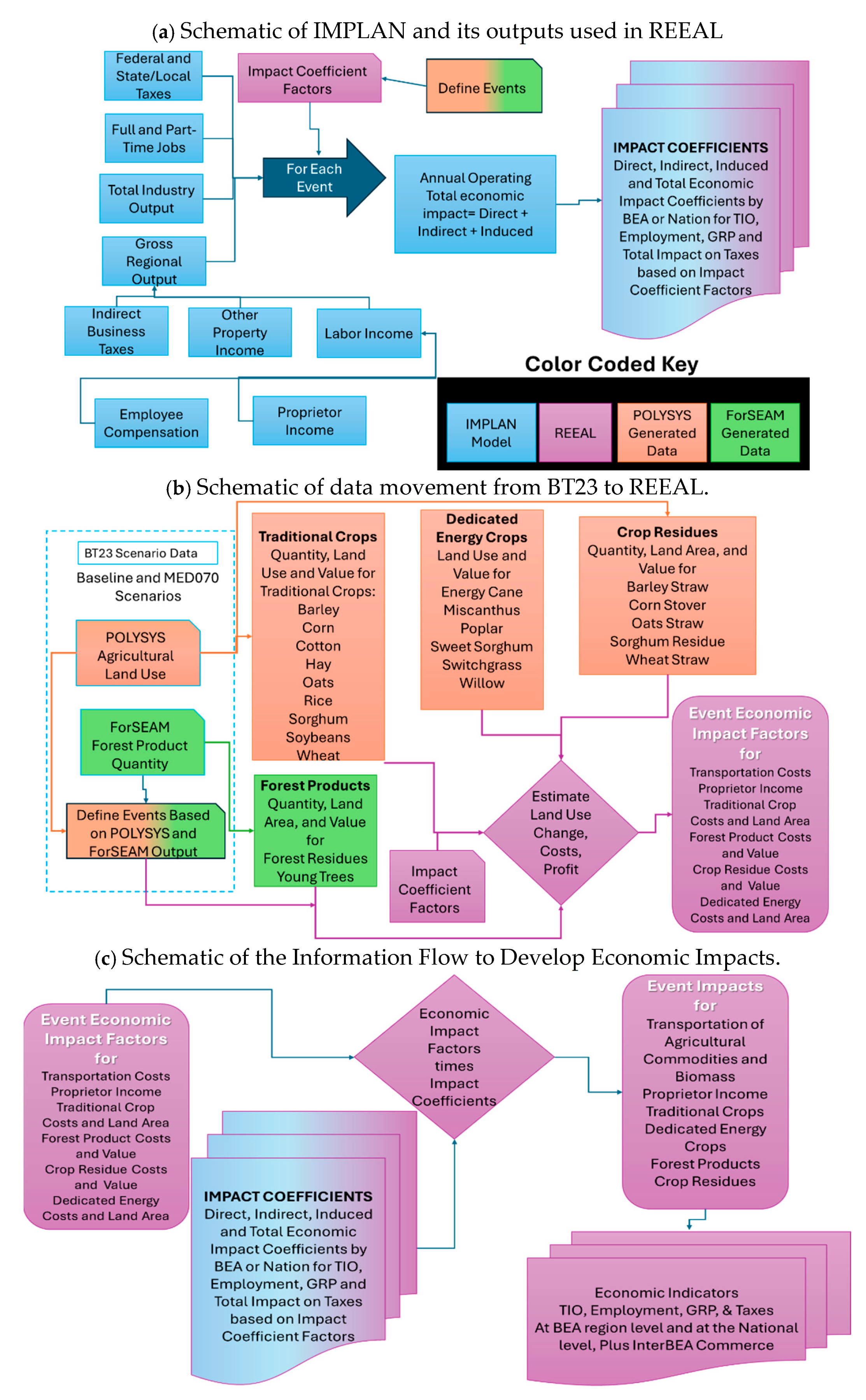
2.1. IMPLAN
2.2. The Events
2.2.1. Cost of Feedstock Production
Traditional Crops
Dedicated Energy Crops
Crop Residues
Forest Products
Transportation Cost
Proprietor Income
2.3. Data from BT23 Economic Modeling Efforts
2.3.1. Output from POLYSYS
2.3.2. Output from ForSEAM
3. Results
3.1. Baseline Scenario Results
3.2. MED070 Biomass Scenario Results
4. Discussion
4.1. A Comparison on the Economic Benefits of Biomass
4.2. Supply Chain Areas
- Biomass—growing and harvesting of dedicated energy crops, collection of crop residues and forest residues and other forest products and transportation of biomass 59 km;
- Transportation—movement from land to facility beyond 59 km;
- Pre-processing—densification, size reduction, and repackaging;
- Transportation—movement from preprocessing to conversion facility;
- Conversion—conversion of biomass to products such as fuel or chemicals, government loans and subsidies;
- Transportation—transportation to users;
- Purchase—use of product, government subsidies.
5. Conclusions
Author Contributions
Funding
Data Availability Statement
Acknowledgments
Conflicts of Interest
Copyright Statement
Abbreviations
| ABP | Analysis by Parts |
| ASD | Agricultural Statistical District |
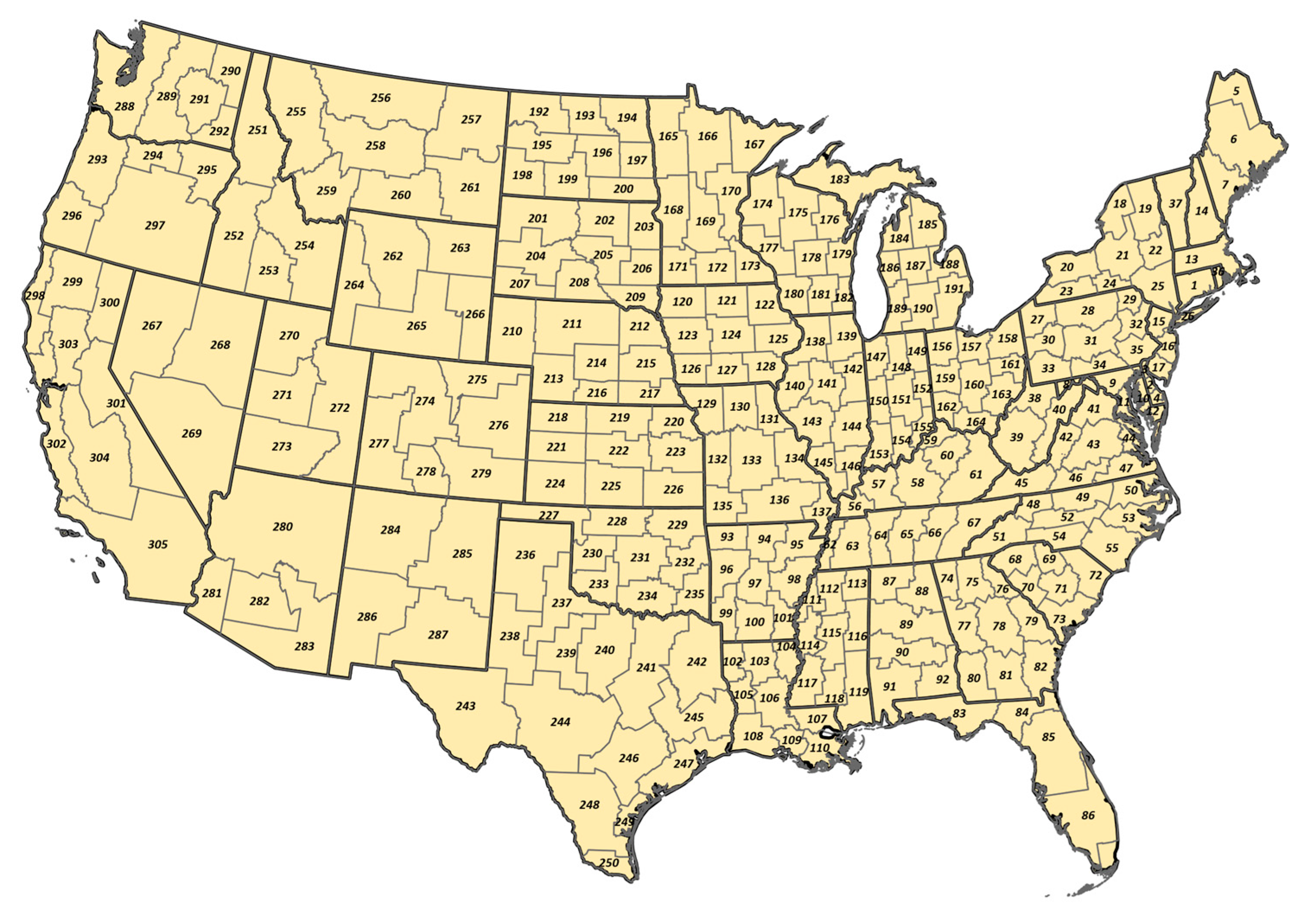
| BEA | Bureau of Economic Analysis Regions |
| BETO | Bioenergy Technologies Office |
| BioFLAME | Biofuels Facility Location Analysis Modeling Endeavor |
| BT23 | Billion-Ton 2023 Report |
| CRD | Crop Reporting District |
| EIO-LCA | Environmental Input-Output/Life Cycle Analysis |
| ForSEAM | Forest Sustainable and Economic Analysis Model |
| GRP | Gross Regional Production |
| IMPLAN | Economic analysis Software |
| KDF | Bioenergy Knowledge Discovery network |
| MaxEnt | Maximum Entropy |
| MED000 | POLYSYS Baseline with no biomass production |
| MED070 | Mature-Market Medium scenario (MED070) with a biomass price of USD 77.14 per dry metric ton (USD 70 per dry ton), along with a wood residue price of USD 44.08 per dry metric ton (USD 40 per dry ton) |
| ORIBAS | Oak Ridge Integrated Bioenergy Analysis System |
| ORCBS | Oak Ridge County-Level Biomass Supply Database |
| ORDEC | Oak Ridge Competitive Electricity Dispatch |
| ORNL | Oak Ridge National Laboratory |
| POLYSYS | Policy System |
| REEAL | Renewable Energy Economic Analysis Layers |
| TIO | Total Industry Output |
Appendix A
| Citation | Models Used | Description and Findings |
|---|---|---|
| [37] | IMPLAN | Sustainable conversion of new amounts of woody biomass to power, after considering accessibility 8 thresholds and extrapolated to potential impacts in the U.S. economy, could translate into new economic contributions in the range of USUSD 5.50 billion to USUSD 21.98 billion per year |
| [38] | (MaxEnt) and an I-O model of Pennsylvania based on IMPLAN | 65 industrial sites were identified. A case study was conducted for forest biomass to pellet fuel in the U.S. Mid-Atlantic region. The socio-economic impacts assessment indicates that the one-year construction of a medium-size pellet fuel facility (75,000 dry tons/year) could create 127 jobs, USD 8.78 million of labor income, while the operation could create 202 jobs, USD 10.52 million of labor income, USD 14.66 million of value added, and USD 33.61 million of output in total per year for the state-level economy. Used industry output, value added, employment, and labor income variables from the I–O model. |
| [39] | IMPLAN | Our input–output model utilizing the IMPLAN software requires data on (1) annual available almond biomass residue; (2) almond acreage in the studied counties; (3) biomass to biochar conversion rates; (4) biochar production costs; and (5) possible biochar selling prices. Examine employment and labor income impacts. |
| [40] | Comparison of JEDI with IMPLAN | This paper calculates the impact on job, income and output creation of a new solar power plant in an input–output framework. |
| [41] | IMPLAN | Used Employment, Labor Income, Total Value Added and output as economic indicators. For example, 100 percent distribution of available woody biomass for bio-oil facilities would generate 5932 full- and part-time jobs with USUSD 700 million of economic output. |
| [42] | IMPLAN | Study objectives were to describe the main economic impacts of developing bioenergy and to specifically quantify the economic impacts on Mississippi’s economy of logging residue recovery, electricity generation from woody biomass, and construction and operation of a biofuel facility. Variables used to measure the impact include output, value added, employment, and income. |
| [43] | IMPLAN and JEDI | A 147 MW wind farm near Weatherford generated an estimated USUSD 27 million in local spending and created 188 jobs during the construction phase. Once operational, the wind farm supports an estimated 13 jobs directly at the wind farm, including technicians and management. Additional estimates show that USUSD 1.7 million continues to be spent annually in the local economy, with over USUSD 600,000 in additional property tax revenue and almost USUSD 400,000 in direct land lease payments to landowners. The model estimates that the combined direct and induced impact annually is over USUSD 25 million. |
| [44] | IMPLAN | The estimated impacts of residue procurement and electricity production on the region’s employment, value added, and output for selected counties in East Texas. The impact assessment was based on current power generation and distribution systems as of 2007 with fossil fuel replacement with woody biomass in power generation. Value-added impact of USD 216M or almost 60% of the total current value-added generated by the logging industry would be added to the economy. Residue procurement would account for less than one-third of the total impacts on value added and output. |
| [45] | IMPLAN | 24 counties make up the hardwood fiber shed for a recently closed pulp mill. Three alternatives were examined in revitalizing the impacted economy by using the surplus fiber and creating new opportunities for the displaced workforce. Results from a multiregional input–output analysis revealed spillover economic opportunities beyond the impacted areas. |
| Item/Crop Number ( ) | Corn (1) | Sorghum (2) | Oats (3) | Barley (4) | Wheat (5) |
| LABOR | 102.01 | 64.52 | 49.77 | 58.07 | 51.27 |
| SEED | 171.22 | 29.11 | 52.66 | 56.34 | 59.33 |
| FUEL | 159.68 | 90.76 | 81.99 | 88.78 | 93.92 |
| LUBRICANTS | 4.82 | 13.29 | 12.31 | 13.32 | 14.09 |
| REPAIRS | 136.95 | 65.21 | 51.92 | 60.29 | 59.87 |
| FERTILIZER N | 115.79 | 53.89 | 87.57 | 94.00 | 77.42 |
| FERTILIZER P | 27.38 | 2.92 | 23.33 | 15.86 | 33.16 |
| FERTILIZER K | 17.77 | 1.61 | 19.50 | 7.34 | 21.60 |
| OTHER FERTILIZER | 46.46 | 39.46 | 17.74 | 40.70 | 34.87 |
| HERBICIDE | 119.77 | 63.78 | 3.98 | 12.40 | 17.17 |
| INSECTICIDE | 63.21 | 2.97 | 1.33 | 2.50 | 1.06 |
| OTHER CHEMICAL | 0.00 | 0.00 | 0.00 | 0.00 | 4.79 |
| IRRIGATION | 0.00 | 0.00 | 0.00 | 0.00 | 0.00 |
| OTHER COSTS | 2.87 | 0.00 | 0.00 | 0.00 | 0.57 |
| HOUSING | 22.17 | 8.06 | 5.81 | 7.39 | 6.82 |
| INSURANCE | 28.96 | 18.24 | 16.41 | 18.01 | 17.57 |
| INTEREST | 82.26 | 66.13 | 58.84 | 65.41 | 64.10 |
| DEPRECIATION | 165.29 | 80.38 | 67.01 | 76.18 | 78.63 |
| TOTAL | 1266.59 | 600.32 | 550.16 | 616.60 | 636.25 |
| Item/Crop Number ( ) | Soybeans (6) | Cotton (7) | Rice (8) | Hay (12) | |
| LABOR | 76.48 | 127.68 | 196.37 | 217.23 | |
| SEED | 146.76 | 218.02 | 209.99 | 28.94 | |
| FUEL | 108.33 | 174.43 | 316.02 | 314.34 | |
| LUBRICANTS | 16.26 | 26.17 | 47.39 | 10.25 | |
| REPAIRS | 76.97 | 157.23 | 283.11 | 172.31 | |
| FERTILIZER N | 2.42 | 75.22 | 221.90 | 11.42 | |
| FERTILIZER P | 33.29 | 38.75 | 11.91 | 31.14 | |
| FERTILIZER K | 50.56 | 29.68 | 41.96 | 52.61 | |
| OTHER FERTILIZER | 59.43 | 47.35 | 5.91 | 27.45 | |
| HERBICIDE | 48.28 | 88.59 | 178.51 | 73.69 | |
| INSECTICIDE | 0.00 | 147.32 | 99.46 | 25.75 | |
| OTHER CHEMICAL | 0.12 | 33.38 | 3.73 | 0.37 | |
| IRRIGATION | 0.00 | 0.00 | 0.00 | 0.00 | |
| OTHER COSTS | 0.00 | 330.18 | 143.89 | 0.00 | |
| HOUSING | 9.14 | 16.56 | 15.99 | 24.09 | |
| INSURANCE | 21.82 | 34.22 | 94.54 | 42.18 | |
| INTEREST | 79.39 | 122.84 | 334.88 | 82.06 | |
| DEPRECIATION | 95.63 | 136.82 | 357.54 | 165.14 | |
| TOTAL | 824.89 | 1804.44 | 2563.10 | 1278.97 |
| Item | Switchgrass | Miscanthus | Sweet Sorghum | Energy Cane | Poplar | Willow |
|---|---|---|---|---|---|---|
| LABOR | 5.04 | 14.18 | 48.09 | 17.05 | 9.24 | 7.36 |
| SEED | 16.65 | 46.97 | 62.20 | 219.40 | 37.19 | 121.58 |
| FUEL | 2.64 | 7.04 | 35.29 | 12.90 | 5.91 | 5.39 |
| LUBRICANTS | 0.40 | 1.06 | 5.31 | 1.93 | 0.89 | 0.82 |
| REPAIRS | 5.88 | 15.52 | 41.64 | 14.16 | 7.22 | 7.83 |
| N FERTILIZER | 0.00 | 0.00 | 447.68 | 0.00 | 35.24 | 23.33 |
| P FERTILIZER | 6.89 | 18.06 | 151.50 | 17.59 | 0.00 | 0.00 |
| K FERTILIZER | 9.02 | 27.16 | 294.65 | 12.01 | 9.02 | 0.00 |
| OTHER FERTILIZER | 9.66 | 23.35 | 95.23 | 21.77 | 24.59 | 0.00 |
| HERBICIDE | 19.37 | 51.10 | 67.78 | 257.24 | 21.99 | 14.97 |
| INSECTICIDE | 0.00 | 0.00 | 0.00 | 0.00 | 4.97 | 0.00 |
| OTHER CHEMICALS | 0.00 | 0.00 | 0.00 | 0.00 | 0.00 | 0.00 |
| NUTRIENT REPLACEMENT | 238.11 | 215.11 | 0.00 | 40.45 | 0.00 | 0.00 |
| OTHER COSTS | 0.00 | 0.00 | 0.00 | 81.77 | 36.89 | 0.00 |
| HOUSING | 1.09 | 2.92 | 7.07 | 2.77 | 1.33 | 0.96 |
| INSURANCE | 0.37 | 0.99 | 2.35 | 0.94 | 0.44 | 0.32 |
| INTEREST | 1.46 | 4.00 | 4.70 | 2.40 | 1.58 | 15.35 |
| DEPRECIATION | 5.19 | 13.71 | 36.18 | 14.88 | 6.10 | 5.66 |
| HARVEST COST | 149.05 | 187.31 | 0.00 | 405.99 | 344.09 | 401.82 |
| AVERAGE PER-ACRE COST | 470.83 | 628.49 | 1299.65 | 1123.24 | 546.70 | 605.38 |
References
- Griffin, M.B. Opening pathways for the conversion of woody biomass into sustainable aviation fuel via catalytic fast pyrolysis and hydrotreating. Green Chem. 2024, 26, 9758–9781. [Google Scholar] [CrossRef]
- Canabarro, N.; Soares, J.F.; Anchieta, C.G.; Kelling, C.S.; Mazutti, M.A. Thermochemical processes for biofuels production from biomass. Sustain. Chem. Process. 2013, 1, 10. [Google Scholar] [CrossRef]
- Board, B.R. Sustainable Aviation Fuel Grand Challenge. 2024. Available online: https://biomassboard.gov/sustainable-aviation-fuel-grand-challenge (accessed on 15 December 2024).
- Perlack, R.D. Biomass as Feedstock for a Bioenergy and Bioproducts Industry: The Technical Feasibility of a Billion-Ton Annual Supply; Oak Ridge National Laboratory: Oak Ridge, TN, USA, 2005. [Google Scholar] [CrossRef]
- U.S. Department of Energy; Perlack, R.D.; Stokes, B.J. U.S. Billion-Ton Update: Biomass Supply for a Bioenergy and Bioproducts Industry; Oak Ridge National Laboratory: Oak Ridge, TN, USA, 2011; 227p. Available online: https://www.energy.gov/eere/bioenergy/articles/us-billion-ton-update-biomass-supply-bioenergy-and-bioproducts-industry (accessed on 15 October 2024).
- U.S. Department of Energy. 2016 Billion-Ton Report: Advancing Domestic Resources for a Thriving Bioeconomy, Volume 1: Economic Availability of Feedstocks; Oak Ridge National Laboratory: Oak Ridge, TN, USA, 2016. Available online: https://info.ornl.gov/sites/publications/Files/Pub62368.pdf (accessed on 6 June 2024).
- U.S. Department of Energy; Efroymson, R.A.; Langholtz, M.H.; Johnson, K.E.; Stokes, B.J. 2016 Billion-Ton Report: Advancing Domestic Resources for a Thriving Bioeconomy, Volume 2: Environmental Sustainability Effects of Select Scenarios from Volume 1; Oak Ridge National Laboratory: Oak Ridge, TN, USA, 2017. [Google Scholar] [CrossRef]
- U.S. Department of Energy; Langholz, M.H. 2023 Billion-Ton Report: An Assessment of U.S. Renewable Carbon Resources; Oak Ridge National Laboratory: Oak Ridge, TN, USA, 2024. Available online: https://bioenergykdf.ornl.gov/document/2023-billion-ton-report (accessed on 6 June 2024).
- U.S. Department of Agriculture. Building a Resilient Biomass Supply A Plan to Enable the Bioeconomy in America; U.S. Department of Agriculture: Washington, DC, USA, 2024. Available online: https://www.usda.gov/sites/default/files/documents/biomass-supply-chain-report.pdf (accessed on 7 December 2024).
- Moore, G. The Analysis of Economic Indicators. Sci. Am. 1975, 232, 17–23. Available online: https://www.jstor.org/stable/24949702 (accessed on 28 February 2025). [CrossRef]
- Olsen, D.; Lindall, A.l. IMPLAN Users Manual; MIG: St. Paul, MN, USA,, 1999. [Google Scholar]
- The Investopedia Team. Economic Indicator: Definition and How to Interpret. 2023. Available online: https://www.investopedia.com/terms/e/economic_indicator.asp#toc-what-is-the-most-important-economic-indicator (accessed on 22 December 2023).
- English, B.; Menard, R.; Wilson, B. The Economic Impact of a Renewable Biofuels/Energy Industry Supply Chain Using the Renewable Energy Economic Analysis Layers Modeling System. Front. Energy Res. Sect. Bioenergy Biofuels 2022, 10, 780795. [Google Scholar] [CrossRef]
- Davis, M.; Lambert, L.H.; Jacobson, R.; Rossi, D.; Brandeis, C.; Fried, J.; English, B.; Abt, R.; Abt, K.; Nepal, P.; et al. Chapter 4: Biomass from the Forested Land Base. In 2023 Billion-Ton Report; Langholtz, M.H., Ed.; Oak Ridge National Laboratory: Oak Ridge, TN, USA, 2024. [Google Scholar] [CrossRef]
- U.S. Department of Transportation; Federal Aviation Administration. Center of Excellence for Alternative Jet Fuels and Environment. In FAA Center of Excellence for Alternative Jet Fuels & Environment: Annual Technical Report 2021: For the Period October 1, 2020–September 30, 2021; Volume 1, Repository and Open Access Science Portal: Washington, DC, USA, 2022. Available online: https://rosap.ntl.bts.gov/view/dot/65765 (accessed on 15 January 2025).
- IMPLAN Model. 2019 Data, Using Inputs Provided by User and IMPLAN Group LLC, Huntersville, NC, 28078. 2024.
- IMPLAN Group LLC. IMPLAN System (Data and Software). Available online: www.IMPLAN.com (accessed on 19 October 2024).
- Clouse, C. ABP: Introduction to Analysis-by-Parts. 2021. Available online: https://support.implan.com/hc/en-us/articles/360044985833-IMPLAN-Report-ToolkitAN-Report-Toolkit–IMPLAN-Support (accessed on 15 May 2021).
- Hellwinckel, C.; de la Torre Ugarte, D.G.; Field, J.L.; Langholtz, M.H. Chapter 5: Biomass from Agriculture. In 2023 Billion-Ton Report; Langholtz, M.H., Ed.; Oak Ridge National Laboratory: Oak Ridge, TN, USA, 2024; pp. 99–125. [Google Scholar] [CrossRef]
- Lambert, L.H.; English, B.C.; Menard, R.J.; Lambert, D.M. Regional Woody Biomass Supply and Economic Impacts from Harvesting in the Southern U.S. Energy Econ. 2016, 60, 151–161. [Google Scholar] [CrossRef]
- Habas, C. Tax Deductions for Building Fences. 2020. Available online: https://pocketsense.com/tax-deductions-building-fences-12087437.html (accessed on 4 October 2024).
- English, B.C. The Economic Feasibility of Crop Residues as Auxiliary Fuel in Coal-fired Power Plantsr. Am. J. Agric. Econ. 1981, 63, 636–644. [Google Scholar] [CrossRef]
- Larson, J.A. Cost Evaluation of Alternative Switchgrass Producing, Harvesting, Storing, and Transporting Systems and Their Logistics in the Southeastern USA. Agric. Financ. Rev. 2010, 70, 184–200. [Google Scholar] [CrossRef]
- U.S. Energy Information Administration; Independant Statistics and Analysis. Gasoline and Diesel Fuel Update. In Petroleum and Other Liquids; U.S. Energy Information Administration: Washington, DC, USA, 2024. Available online: https://www.eia.gov/petroleum/gasdiesel/ (accessed on 8 November 2024).
- United State Prime Rate. 2024. Available online: https://fedprimerate.com/ (accessed on 2 December 2024).
- U.S. Bureau of Labor Statistics. 53-7121 Tank Car, Truck, and Ship Loaders. In Occupational Employment and Wage Statistics; U.S. Bureau of Labor Statistics: Washington, DC, USA, 2023. Available online: https://www.bls.gov/oes/2023/may/oes537121.htm (accessed on 15 December 2024).
- U.S. Department of Agriculture, Agricultural Marketing Service. Grain Transportation Report; U.S. Department of Agriculture: Washington, DC, USA, 2024. Available online: https://agtransport.usda.gov/Truck/Quarterly-Grain-Truck-Rates/xs2f-6ba7 (accessed on 1 October 2024).
- Commercial Truck Trader. Used 2023 FREIGHTLINER Conventional-Day Cab-Cascadia 126. Newsletter. Pine Bluff, AR, USA. 2024. Available online: https://www.commercialtrucktrader.com/listing/2023-FREIGHTLINER-Cascadia+126-5033840779#sid=683604 (accessed on 11 November 2024).
- Kaufman Trailers of SC; SC Sales. 2024 Kaufman 50 Ton Detachable Lowboy Trailer. 2024. Available online: https://www.truckpaper.com/listing/for-sale/31869795/2024-kaufman-50-ton-detachable-lowboy-trailer-lowboy-trailers-semi-trailers?print=1 (accessed on 11 November 2024).
- Kenworth Sales Company Chesapeake; Commercial Truck Trader. Used 2020 KENWORTH Dump Truck, Contractor Truck, Chipper Truck—T370. 2024. Available online: https://www.commercialtrucktrader.com/ (accessed on 2 October 2024).
- de la Torre Ugarte, D.G. Biomass and Bioenergy Applications of the POLYSYS Modeling Framework. Biomass Bioenergy 2000, 18, 291–308. [Google Scholar] [CrossRef]
- Walsh, M.D. The Economic Impacts of Bioenergy Crop Production on U.S. Agric. Environ. 2003, 24, 313–333. [Google Scholar]
- Stokes, B.J. TimberHarvestCosts_Rev.xlsx; U.S. Forest Service: Washington, DC, USA, 2014. [Google Scholar]
- U.S. Department of Agriculture; National Agricultural Statistics Service. Crop VAlues 2023 Summary; U.S. Department of Agriculture: Washington, DC, USA, 2024; Available online: https://downloads.usda.library.cornell.edu/usda-esmis/files/k35694332/g158d382b/cn69nq74z/cpvl0224.pdf (accessed on 15 January 2025).
- U.S. Department of Agriculture; National Agricultural Statistics Service. Crop Production 2024 Summary; U.S. Department of Agriculture: Washington, DC, USA, 2025; Available online: https://downloads.usda.library.cornell.edu/usda-esmis/files/k3569432s/nk324887m/qn59s0097/cropan25.pdf (accessed on 31 January 2025).
- U.S. Environmental Protection Agency. RIN Trades and Price Information; EPA: Washington, DC, USA, 2022. [Google Scholar]
- Dahal, R.P.; Francisco, X.; Aguilar, R.G.; Becker, D.; Abt, K.L. Localized economic contributions of renewable wood-based biopower generation. Energy Econ. 2020, 91, 104913. [Google Scholar] [CrossRef]
- Zhang, X.; Wang, J.; Strager, M.P. Industrial DevelopImpacts of Forest Biomass for Bioenergy: A Data-Driven Holistic Analysis Frameworkment and Economic. Resour. Conserv. Recycl. 2022, 182, 106296. [Google Scholar] [CrossRef]
- Nematian, M.; Ng’ombe, J.N.; Keske, C. Sustaining agricultural economies: Regional economic impacts of biochar production from waste orchard biomass in California’s Central Valley. Environ. Dev. Sustain. 2024, 26, 30701–30721. [Google Scholar] [CrossRef]
- Bae, J.; Dall’erba, S. The economic impact of a new solar power plantin Arizona: Comparing the input-output results generatedby JEDI vs. IMPLAN. Reg. Sci. Policy Pract. 2016, 8, 61–74. [Google Scholar] [CrossRef]
- Joshi, O.; Grebner, D.L.; Henderson, J.E.; Grado, S.C.; Munn, I.A. Input–Output Modeling of Wood-Based Bioenergy Industries in Mississippi. For. Prod. J. 2012, 62, 528–537. [Google Scholar] [CrossRef]
- Perez-Verdin, G.; Grebner, D.L.; Munn, I.A.; Sun, C.; Gardo, S.C. Economic Impacts of Woody Biomass Utilization for bioenergy in Mississippi. For. Prod. J. 2008, 58, 75–83. [Google Scholar]
- Greene, J.S.; Geisken, M. Socioeconomic Impacts of Wind Farm Development: A Case Study of Weatherford, Oklahoma. Energy Sustain. Soc. 2013, 3, 2. [Google Scholar] [CrossRef]
- Gan, J.; Smith, C. Co-benefits of utilizing logging residues for bioenergy production: The case for East Texas, USA. Biomass Bioenergy 2007, 31, 623–630. [Google Scholar] [CrossRef]
- Poudyal, N.C.; Omkar Joshi, A.M. Prospects of Wood-Based Energy Alternatives in Revitalizing the Economy Impacted by Decline in the Pulp and Paper Industry. For. Prod. J. 2017, 67, 427–434. [Google Scholar] [CrossRef]


| Event Category | Different Events Identified | Baseline | MED070 |
|---|---|---|---|
| TRADITIONAL CROPS | 9—Barley, Corn, Cotton, Hay, Oats, Rice, Sorghum, Soybean, and Wheat | Yes | Yes |
| DEDICATED ENERGY CROPS | 7—Energy Cane, Miscanthus, Hybrid Poplar, Sweet Sorghum, Switchgrass, Willows, and Intensified Pasture | No | Yes |
| CROP RESIDUES | 5—Barley Straw, Corn Stover, Oat Straw, Sorghum Residue, and Wheat Straw | No | Yes |
| FOREST PRODUCTS | 6—Forest Residue (Machinery, Labor, and Proprietor Income) and Young Trees (Machinery, Labor, and Proprietor Income) | No | Yes |
| TRANSPORTATION | 5—Transportation for Traditional Crops, Herbaceous Dedicated Energy Crops, Woody Dedicated Energy Crops, Crop Residues, and Forest Products | Partial—only Traditional Crops | Yes |
| PROPRIETOR INCOME | 4—Proprietor Income for Traditional Crops, Dedicated Energy Crops, Crop Residues, and Forest Products | Partial—only Traditional Crops | Yes |
| Budget Cost Item | Impacted IMPLAN Industry Sector |
|---|---|
| Depreciation | (456) Accounting, Tax Preparation, Bookkeeping, & Payroll Services |
| Fertilizer K | (19) Support Activities for Agriculture & Forestry |
| Fertilizer N | (19) Support Activities for Agriculture & Forestry |
| Fertilizer P | (19) Support Activities for Agriculture & Forestry |
| Fuel | (408) Retail—Gasoline Stores |
| Herbicide | (19) Support Activities for Agriculture & Forestry |
| Housing | (448) Tenant-Occupied Housing |
| Insecticide | (19) Support Activities for Agriculture & Forestry |
| Insurance | (444) Insurance Carriers, except Direct Life |
| Interest | (439) Non-depository Credit Intermediation & Related Activities |
| Irrigation | (49) Water, Sewage, & Other Systems |
| Labor | (19) Support Activities for Agriculture & Forestry |
| Lubricants | (408) Retail—Gasoline Stores |
| Other Chemical | (19) Support Activities for Agriculture & Forestry |
| Other Costs | (19) Support Activities for Agriculture & Forestry |
| Other Fertilizer | (19) Support Activities for Agriculture & Forestry |
| Repairs | (515) Commercial & Industrial Machinery & Equipment Repair & Maintenance |
| Seed | (405) Retail—Building Material & Garden Equipment & Supplies Stores |
| Labor | Proprietor Income |
| Pasture | (19) Support Activities for Ag/Forestry |
| Transportation | (417) Truck Transportation |
| Logging | (16) Commercial Logging |
| Chipping | (408) Retail—Gasoline Stores and (515) Commercial & Industrial Machinery & Equipment Repair & Maintenance |
| Harvest | (19) Support Activities for Ag/Forestry; (408) Retail—Gasoline Stores; (439) Nondepository Credit Intermediation & Related Activities; (444) Insurance Carriers, except Direct Life; (456) Accounting, Tax Preparation, Bookkeeping, & Payroll Services; (515) Commercial & Industrial Machinery & Eq Repair & Maintenance; and Labor—Employee Compensation |
| Residue Type | Collection Costs | Nutrient Costs | Proprietor Income | Average Yield |
|---|---|---|---|---|
| USD per hectare | Metric Tons/hectare | |||
| Corn Stover | 77.10 | 215.35 | 166.97 | 6.5 |
| Sorghum Residue | 119.77 | 149.08 | 38.28 | 4.3 |
| Oat Straw | 75.94 | 104.67 | 35.04 | 2.9 |
| Barley Straw | 84.83 | 106.45 | 28.00 | 3.1 |
| Wheat Straw | 93.13 | 97.26 | 28.32 | 3.1 |
| Feedstock | Capital Cost for Dump Truck or Semi-Truck with Flatbed Trailer or Hopper a | Weight /Load b | Distance | Transportation Cost | Transportation Cost | |
|---|---|---|---|---|---|---|
| USD | Dry Metric Ton | km | USD/Metric Ton | USD/Metric Ton-Kilometer | ||
| Wood chips | 164,900 | 21.7 b | 59.5 | 14.69 | 0.25 | |
| Baled material | 169,155 | 14.2 b | 59.5 | 22.73 | 0.38 | |
| Traditional Crops | 123,810 | 25.8 c | 59.5 | 9.68 c | 0.16 | |
| Traditional Crop | Traditional Crop Price | Direct | Indirect | Induced | Total |
|---|---|---|---|---|---|
| USD/metric ton | Million USDs | ||||
| BARLEY | 248.48 | 312 | 86 | 141 | 539 |
| CORN | 177.16 | 22,980 | 6776 | 12,169 | 41,924 |
| COTTON | 1807.79 | 6613 | 1453 | 3501 | 11,566 |
| HAY | 190.44 | 16,719 | 5351 | 8533 | 30,603 |
| OATS | 230.11 | 308 | 92 | 160 | 560 |
| RICE | 359.35 | 1533 | 443 | 737 | 2714 |
| SORGHUM | 168.50 | 893 | 229 | 403 | 1525 |
| SOYBEAN | 393.16 | 14,806 | 4820 | 7588 | 27,213 |
| WHEAT | 225.24 | 6784 | 1895 | 3190 | 11,869 |
| TRANSPORTATION | NA | 46,342 | 22,072 | 20,008 | 88,423 |
| PROPRIETOR INCOME | NA | 38,385 | 0 | 30,933 | 69,317 |
| SUBTOTAL | ND | 155,675 | 43,217 | 87,361 | 286,254 |
| INTRABEA COMMERCE | NA | 37,530 | 52,636 | 143,592 | 233,759 |
| TOTAL | ND | 193,205 | 95,854 | 230,953 | 520,012 |
| Event | Direct | Indirect | Induced | Total |
|---|---|---|---|---|
| Number of full- and part-time jobs | ||||
| BARLEY | 4130 | 515 | 934 | 5579 |
| CORN | 283,200 | 38,449 | 77,337 | 398,986 |
| COTTON | 108,548 | 8403 | 23,712 | 140,662 |
| HAY | 220,663 | 31,005 | 54,315 | 305,983 |
| OATS | 4069 | 522 | 1014 | 5605 |
| RICE | 19,341 | 2621 | 4823 | 26,785 |
| SORGHUM | 11,338 | 1388 | 2693 | 15,418 |
| SOYBEAN | 167,915 | 27,671 | 48,407 | 243,994 |
| WHEAT | 86,842 | 11,120 | 20,726 | 118,688 |
| TRANSPORTATION | 282,680 | 126,751 | 128,964 | 541,516 |
| PROPRIETOR INCOME | 0 | 0 | 196,787 | 196,787 |
| SUBTOTAL | 1,188,727 | 248,444 | 559,712 | 2,000,003 |
| INTRABEA COMMERCE | 391,381 | 177,935 | 667,197 | 1,233,919 |
| TOTAL | 1,580,108 | 426,379 | 1,226,909 | 3,233,922 |
| Event Category | Federal | State/Local | Total |
|---|---|---|---|
| Billion USDs | |||
| Traditional Crops | 11,289 | 8359 | 19,647 |
| Energy Crops | 0 | 0 | 0 |
| Residue | 0 | 0 | 0 |
| Forest Feedstock | 0 | 0 | 0 |
| Transportation | 6248 | 4283 | 10,531 |
| Proprietor | 2119 | 1878 | 3997 |
| Subtotal | 19,655 | 14,520 | 34,175 |
| IntraBEA Commerce | 19,082 | 11,474 | 30,556 |
| US Total | 38,738 | 25,993 | 64,731 |
| Biomass Category and Biomass Event | Area Supplying Biomass | Biomass Quantity | Accumulated by Biomass Type | Total Biomass Production |
|---|---|---|---|---|
| Hectares | Dry metric tons | |||
| Dedicated Energy Crops: | ||||
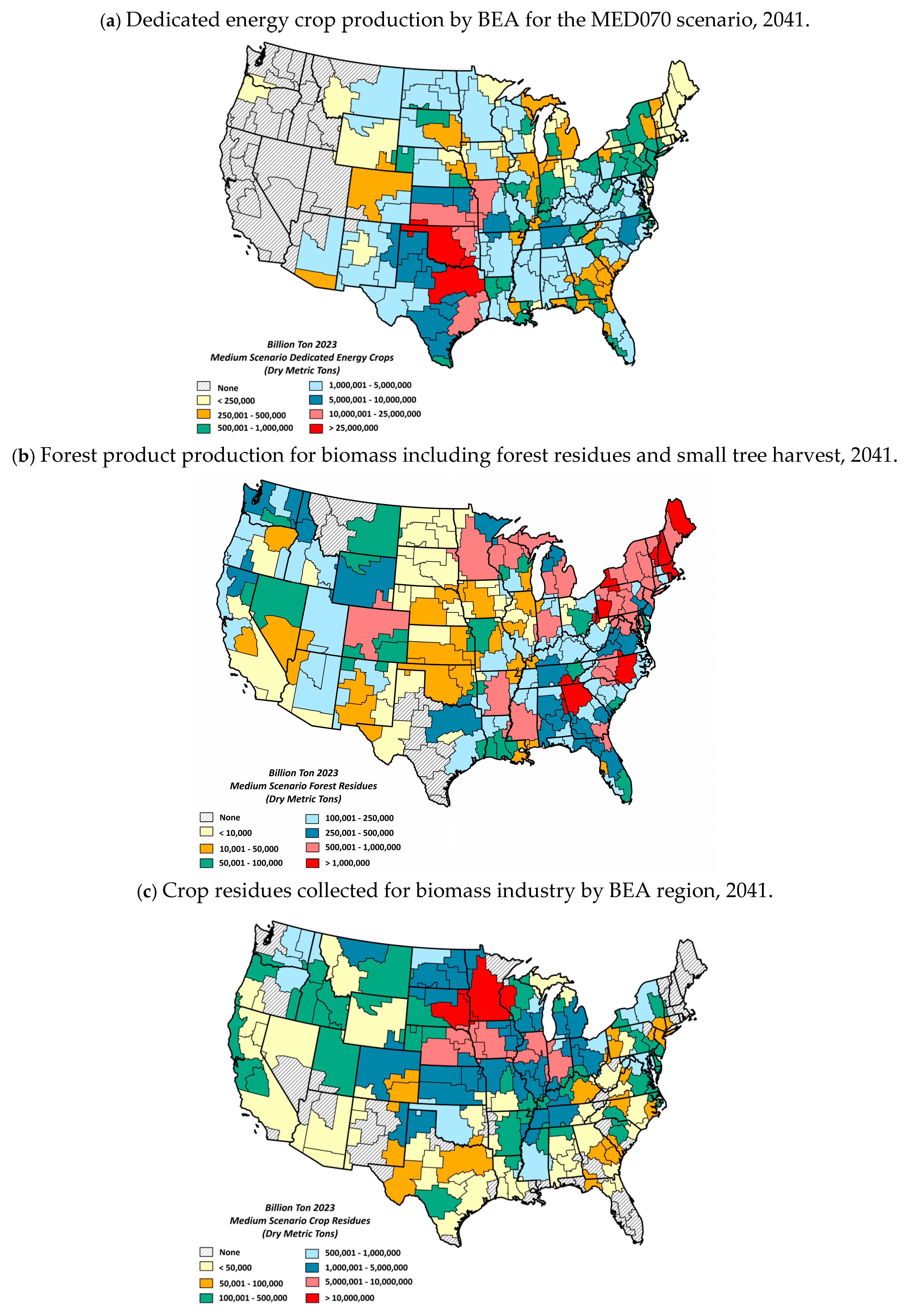
| Energy Cane | 23,550 | 505,317 | 361,205,055 | 564,360,433 |
| Miscanthus | 6,689,879 | 99,985,196 | ||
| Poplars | 438,039 | 4,882,940 | ||
| Biomass Sorghum | 119,014 | 3,176,675 | ||
| Switchgrass | 20,154,485 | 209,050,292 | ||
| Willows | 3,405,308 | 43,604,636 | ||
| Dedicated Energy Crop Land Area Total | 30,830,275 | |||
| Crop Residues: | 477,920 | |||
| Barley Straw | 152,969 | 144,530,629 | 162,306,374 | |
| Corn Stover | 23,019,372 | 9662 | ||
| Oat Straw | 3116 | 1,243,812 | ||
| Sorghum Residue | 275,871 | 16,044,351 | ||
| Wheat Straw | 5,184,093 | 477,920 | ||
| Crop Residue Acreage Total | 28,635,422 | |||
| Forest Products: | ||||
| Forest Residues | 947,438 | 14,936,106 | 40,849,004 | |
| Whole Tree Feedstock | 729,084 | 25,912,897 | ||
| Forest Product Acreage Total | 1,676,522 | |||
| Totals | 61,142,219 | 564,360,433 | ||
| Traditional Crop/Biomass Supply Event | Crop Price | Direct | Indirect | Induced | Total |
|---|---|---|---|---|---|
| USD/metric ton | Million USDs | ||||
| Barley | 272.36 | 318 | 90 | 146 | 553 |
| Corn | 183.85 | 21,416 | 6384 | 11,411 | 39,211 |
| Cotton | 959.01 | 4995 | 1137 | 2643 | 8775 |
| Hay | 190.42 | 16,588 | 5308 | 8471 | 30,367 |
| Oats | 204.8 | 289 | 87 | 151 | 527 |
| Rice | 373.68 | 1460 | 427 | 706 | 2592 |
| Sorghum | 183.06 | 746 | 191 | 336 | 1273 |
| Soybean | 420.71 | 13,313 | 4333 | 6829 | 24,474 |
| Wheat | 258.68 | 5697 | 1589 | 2729 | 10,015 |
| Subtotal Traditional Crops | 64,822 | 19,546 | 33,421 | 117,789 | |
| Barley Straw | 41.88 | 17 | 2 | 11 | 29 |
| Corn Stover | 60.41 | 3526 | 499 | 2820 | 6844 |
| Oat Straw | 43.21 | 1 | 0 | 0 | 1 |
| Sorghum Residue | 41.51 | 38 | 4 | 23 | 65 |
| Wheat Straw | 41.48 | 495 | 62 | 325 | 881 |
| Subtotal Crop Residues | 4076 | 566 | 3179 | 7821 | |
| Residues from Forest Operations | 44.09 | 427 | 30 | 297 | 754 |
| Whole Tree Harvest for Feedstock | 72.62 | 805 | 177 | 541 | 1522 |
| Subtotal Forest Products | 1232 | 206 | 838 | 2276 | |
| Energy Cane | 72.62 | 10 | 2 | 6 | 18 |
| Miscanthus | 72.62 | 1410 | 252 | 889 | 2551 |
| Poplar | 72.62 | 53 | 12 | 32 | 97 |
| Sweet Sorghum | 72.62 | 77 | 13 | 46 | 137 |
| Switchgrass | 72.62 | 4084 | 642 | 2552 | 7277 |
| Willow | 72.62 | 290 | 82 | 138 | 510 |
| Subtotal Dedicated Energy Crops | NA | 5924 | 1003 | 3663 | 10,589 |
| Traditional Plus Biomass Production | ND | 76,053 | 21,321 | 41,101 | 138,475 |
| Transportation | NA | 56,548 | 27,062 | 24,460 | 108,070 |
| Proprietor Income | NA | 66,970 | 0 | 53,328 | 120,298 |
| Subtotal Allocated to BEAs | ND | 199,572 | 91,025 | 201,091 | 491,688 |
| IntraBEA Commerce | NA | 30,390 | 16,723 | 80,378 | 127,490 |
| Total | ND | 229,961 | 107,748 | 281,469 | 619,178 |
| Event | Direct | Indirect | Induced | Total |
|---|---|---|---|---|
| Number of full- and part-time jobs | ||||
| Commodity Production | 1,145,816 | 131,818 | 283,459 | 1,561,093 |
| Transportation | 282,680 | 126,751 | 128,964 | 541,516 |
| Proprietor Income | 0 | 0 | 196,787 | 196,787 |
| Subtotal | 1,428,496 | 258,569 | 609,210 | 2,296,275 |
| IntraBEA Commerce | 487,496 | 217,236 | 886,428 | 1,591,160 |
| Total | 1,915,993 | 475,805 | 1,495,638 | 3,887,435 |
| Event Category | BEA Allocated Taxes | Interstate Commerce | Generated in USA |
|---|---|---|---|
| Million USD | |||
| Federal Taxes: | |||
| Traditional | 10,310 | 11,263 | 21,573 |
| Energy Crops | 1250 | 902 | 2152 |
| Crop Residues | 854 | 1849 | 2703 |
| Timberland | 142 | 121 | 263 |
| Transportation | 7627 | 5823 | 13,450 |
| Proprietor Income | 3631 | 3463 | 7095 |
| Subtotal | 23,815 | 23,421 | 47,235 |
| State/Local Taxes: | |||
| Traditional | 7740 | 6374 | 14,115 |
| Energy Crops | 525 | 631 | 1156 |
| Crop Residues | 418 | 941 | 1359 |
| Timberland | 88 | 73 | 161 |
| Transportation | 5144 | 4046 | 9191 |
| Proprietor Income | 3125 | 2120 | 5245 |
| Subtotal | 17,040 | 14,186 | 31,227 |
| Total Taxes: | |||
| Traditional | 18,050 | 17,637 | 35,687 |
| Energy Crops | 1775 | 1534 | 3309 |
| Crop Residues | 1272 | 2790 | 4062 |
| Timberland | 229 | 194 | 424 |
| Transportation | 12,772 | 9869 | 22,641 |
| Proprietor Income | 6756 | 5584 | 12,340 |
| Total | 40,855 | 37,607 | 78,462 |
| Indicators from Event Categories | Units | 2023 Production a | MED070 Scenario | Baseline | Difference |
|---|---|---|---|---|---|
| Million units | |||||
| Traditional: | |||||
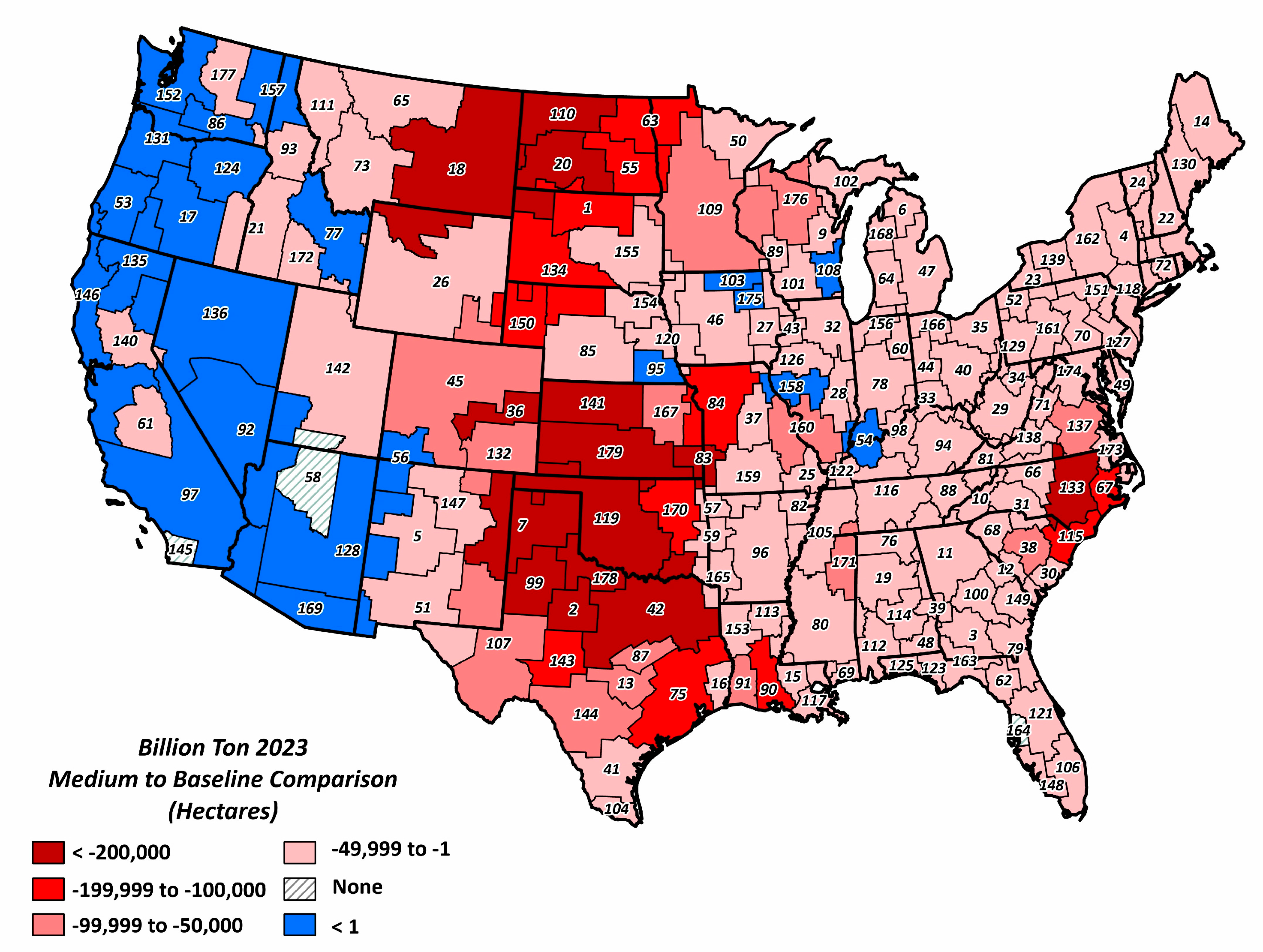
| Land use | Hectares | 123.8 | 111.5 | 122.1 | −10.6 |
| Commodity Value | USD | 172,777 | 180,454 | 170,692 | 9761.3 |
| Transportation Cost b | USD | 5624 | 6113 | 6247 | −134.3 |
| Proprietor Value | USD | Undefined | 50,173 | 36,496 | 13,677.0 |
| Quantity | Metric Tons | 685.1 | 741 | 761 | −20.2 |
| Pastureland: | |||||
| Cropland Pasture | Hectares | 0.0 | 0.8 | 4.0 | −3.2 |
| Permanent Pasture | Hectares | 0.0 | 59.8 | 112.1 | −52.4 |
| Intensified Pasture | Hectares | Undefined | 35.3 | 0.0 | 35.3 |
| Energy Crops: | |||||
| Land use | Hectares | 0 | 30.8 | 0 | 30.8 |
| Commodity Value | USD | Undefined | 172,777 | 0 | 172,777.2 |
| Transportation Cost | USD | Undefined | 782 | 0 | 782.0 |
| Proprietor Value | USD | Undefined | 9126 | 0 | 9126.0 |
| Quantity | Metric Tons | 0 | 755 | 0 | 755.2 |
| Crop Residues: | |||||
| Land use c | Hectares | 0 | 28.6 | 0 | 28.6 |
| Commodity Value | USD | Undefined | 11,787 | 0 | 11,787.3 |
| Transportation Cost | USD | Undefined | 369 | 0 | 368.9 |
| Proprietor Value | USD | Undefined | 4115 | 0 | 4115.0 |
| Quantity | Metric Tons | 0 | 179 | 0 | 178.9 |
| Forest Products: | |||||
| Land use | Hectares | 0 | 1.7 | 0 | 1.7 |
| Commodity Value | USD | Undefined | 2658 | 0 | 2658.1 |
| Transportation Cost | USD | Undefined | 60 | 0 | 60.0 |
| Proprietor Value | USD | Undefined | 261 | 0 | 260.7 |
| Quantity | Metric Tons | USD0 | 45 | 0 | 45.0 |
| Total: | |||||
| Land use | Hectares | 124 | 173 | 122 | 51 |
| Commodity Value | USD | Undefined | 367,676 | 170,692 | 196,984 |
| Transportation Cost | USD | Undefined | 7324 | 6247 | 1077 |
| Proprietor Value | USD | Undefined | 63,675 | 36,496 | 27,179 |
| Quantity | Metric Tons | 0 | 979 | 0 | 979 |
| Full Impact Measures | |||||
| Economic Activity | USD | Unknown | 619,178 | 520,012 | 99,166.1 |
| Employment Impacts | Jobs | Unknown | 3.89 | 3.23 | 0.7 |
| Gross Regional Product | USD | Unknown | 379,273 | 315,437 | 63,836 |
| Tax Collections | USD | Unknown | 75,845 | 64,731 | 11,114 |
Disclaimer/Publisher’s Note: The statements, opinions and data contained in all publications are solely those of the individual author(s) and contributor(s) and not of MDPI and/or the editor(s). MDPI and/or the editor(s) disclaim responsibility for any injury to people or property resulting from any ideas, methods, instructions or products referred to in the content. |
© 2025 by the authors. Licensee MDPI, Basel, Switzerland. This article is an open access article distributed under the terms and conditions of the Creative Commons Attribution (CC BY) license (https://creativecommons.org/licenses/by/4.0/).
Share and Cite
English, B.C.; Menard, R.J.; de la Torre Ugarte, D.G.; Lambert, L.H.; Hellwinckel, C.M.; Langholtz, M.H. Agriculture’s Potential Regional Economic Contributions to the United States Economy When Supplying Feedstock to the Bio-Economy. Energies 2025, 18, 2081. https://doi.org/10.3390/en18082081
English BC, Menard RJ, de la Torre Ugarte DG, Lambert LH, Hellwinckel CM, Langholtz MH. Agriculture’s Potential Regional Economic Contributions to the United States Economy When Supplying Feedstock to the Bio-Economy. Energies. 2025; 18(8):2081. https://doi.org/10.3390/en18082081
Chicago/Turabian StyleEnglish, Burton C., Robert Jamey Menard, Daniel G. de la Torre Ugarte, Lixia H. Lambert, Chad M. Hellwinckel, and Matthew H. Langholtz. 2025. "Agriculture’s Potential Regional Economic Contributions to the United States Economy When Supplying Feedstock to the Bio-Economy" Energies 18, no. 8: 2081. https://doi.org/10.3390/en18082081
APA StyleEnglish, B. C., Menard, R. J., de la Torre Ugarte, D. G., Lambert, L. H., Hellwinckel, C. M., & Langholtz, M. H. (2025). Agriculture’s Potential Regional Economic Contributions to the United States Economy When Supplying Feedstock to the Bio-Economy. Energies, 18(8), 2081. https://doi.org/10.3390/en18082081