Abstract
This paper proposes a fault self-healing recovery strategy for passive low-voltage power station areas (LVPSAs). Firstly, being aware of the typical structure and communication conditions of the LVPSAs, a fog computing load forecasting method is proposed based on a dynamic aggregation of incremental learning models. This forecasting method embeds two weighted ultra-short-term load forecasting techniques of complementary characteristics and mines real-time load to learn incrementally, and thanks to this mechanism, the method can efficiently make predictions of low-voltage loads with trivial computational burden and data storage. Secondly, the low-voltage power restoration problem is overall formulated as a three-stage mixed integer program. Specifically, the master problem is essentially a mixed integer linear program, which is mainly intended for determining the reconfiguration of binary switch states, while the slave problem, aiming at minimizing load curtailment constrained by power flow balance along with inevitable load forecast errors, is cast as mixed integer type-1 Wasserstein distributionally robust optimization. The column-and-constraint generation technique is employed to expedite the model-resolving process after the slave problem with integer variables eliminated is equated with the Karush–Kuhn–Tucker conditions. Comparative case studies are conducted to demonstrate the performance of the proposed method.
1. Introduction
China has launched a magnificent plan to promote intelligent processes for the distribution systems in response to extreme weather and renewable energy consumption. In contrast to the attention-attracting high-voltage distribution network construction, the majority stock of 380 V-below low-voltage power station areas (LVPSAs) remain passive and have lower levels of automation due to prohibitive investment in upgrading the infrastructure. Thus, it is of great significance to explore a capital-efficient scheme to improve the self-healing ability of LVPSAs to power interruption events, which tend to be increasingly intensive with frequent extreme weather.
At this stage, extensive research has been conducted on the fault self-healing of medium-voltage distribution networks [1,2]. However, due to different communication environments, the results achieved cannot fully meet the needs of low-voltage distribution network fault self-healing. Network reconstruction is a common method for distribution networks to achieve fault self-healing. Combined with the structural characteristics of low-voltage distribution networks, the issue of low-voltage network topology reconstruction has also attracted attention. For example, the literature [3] proposes a network reconstruction method for medium- and low-voltage distribution network coordination based on neural networks for the problem of phase-to-phase load balancing. The literature [4] proposes a multi-objective tie switch optimization configuration method for low-voltage photovoltaic accommodation problems, but none of them consider the change in load demand during low-voltage fault repair and the difficulty in obtaining low-voltage line parameters.
Low-voltage fault repair time generally lasts for several hours. Short-term load demand changes have a significant impact on fault recovery strategies [5]. Current short-term load forecasting technologies mainly include traditional data-driven, artificial intelligence, and hybrid forecasting methods. Traditional data-driven methods are represented by methods such as the autoregressive integrated moving average (ARIMA) and modal decomposition. Artificial intelligence methods [6,7] include the long short-term memory network (LSTM) [8,9], convolutional neural network [10], and an adversarial neural network method [11]. Note that model training for these methods often relies on large numbers of samples and computing resources. In contrast, incremental learning methods developed in recent years [12,13] can obtain high-precision short-term load forecasting with less computing resources by supplementing real-time samples. From the perspective of communication and computing power costs, incremental learning prediction has good potential for application in low-voltage load prediction problems with a large number of nodes and relatively simple nature components.
From the above literature summary, it is evident that research on the self-healing and recovery of LVPSAs is still very limited. Issues such as communication technology and the configuration of self-healing equipment for LVPSAs remain in their early stages. Existing self-healing techniques developed for medium-voltage distribution systems often rely on precise line parameters. Meanwhile, short-term load forecasting methods, despite leveraging advanced intelligent techniques, typically require extensive historical load records and long training times. In this regard, it is necessary to consider communication cost and quality to propose efficient load prediction and self-healing methods which are viable to deploy on the lightweight computing hardware.
Being aware of the typical structure of LVPSAs and investment limitations of complex communication infrastructure, this paper proposes a fault self-healing strategy for LVPSAs based on fog computing architecture. In comparison with the existing literature, the main contributions of this paper are highlighted as follows:
- A fog computing load forecasting method, used to offer load demand inputs of the self-healing strategy, is proposed based on a dynamic aggregation of incremental learning models. This forecasting method embeds two weighted ultra-short-term load forecasting techniques with complementary characteristics and mines real-time load to learn incrementally.
- A line-parameter-free self-healing strategy for a faulted LVPSA is formulated as a three-stage mixed integer program, which of the slave subproblem is forged as a type-1 Wasserstein distributionally robust optimization (p-1WDRO) accounting for inevitable load forecast errors in a data-driven manner.
- An algorithm to expedite the model-resolving process is proposed by means of the column-and-constraint generation algorithm. To this end, integer variables involved in the slave problem are eliminated a priori to help derive the equivalent Karush–Kuhn–Tucker conditions with the embedded p-1WDRO problem.
The rest of this paper is organized as follows. Section 2 describes the fog communication framework and operating hypotheses designed for applying the proposed LVPSA self-healing strategy. Section 3 elaborates on the ultra-short-term load forecast method. And, the proposed LVPSA self-healing strategy, along with the resolving algorithm, is described in Section 4, which is followed by case studies and conclusions making up Section 5 and Section 6, respectively.
2. Framework and Hypotheses
2.1. Concept and Hypotheses
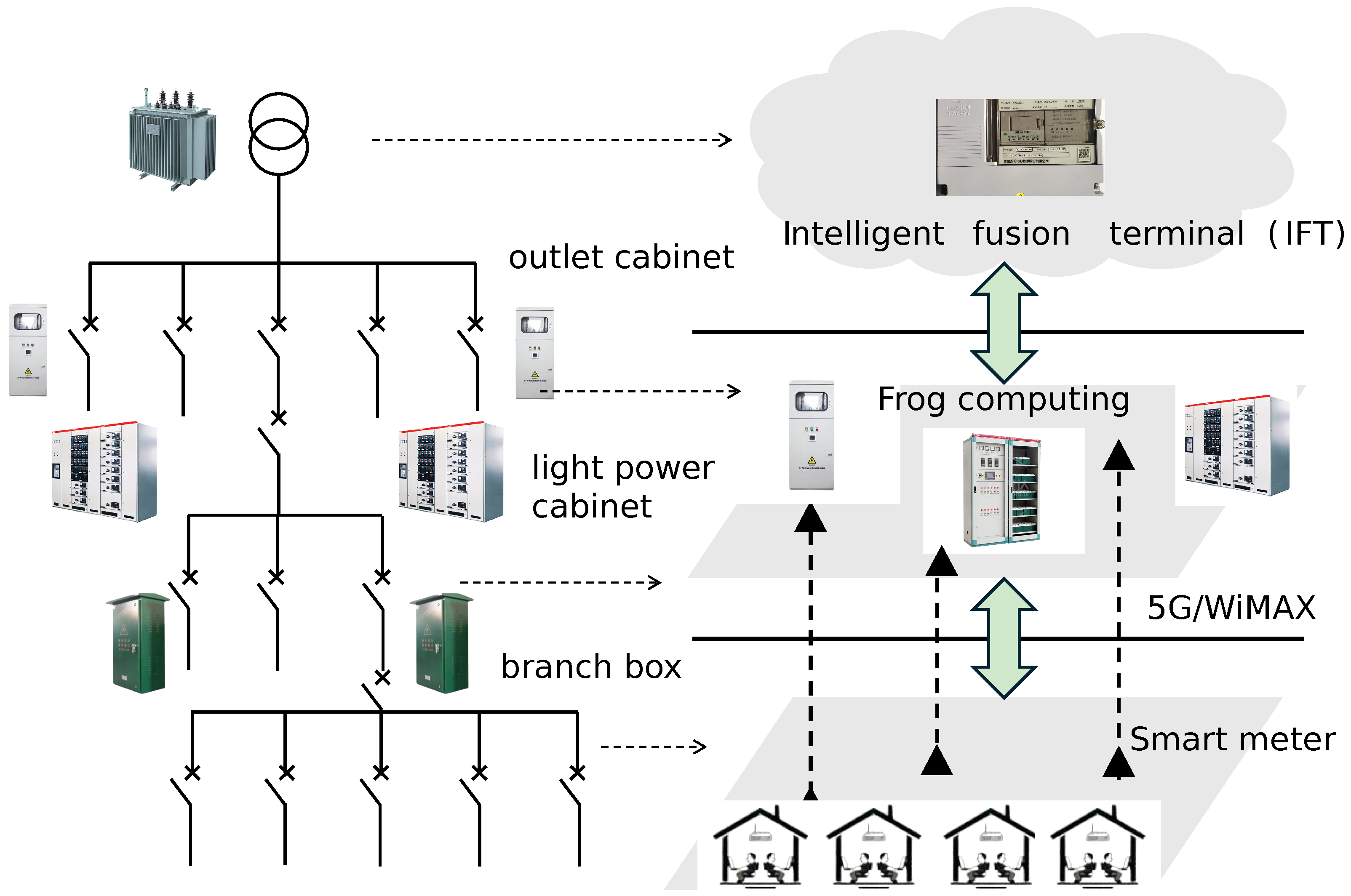
To avoid ambiguity with respect to the current research status of renewable energy penetrated distribution networks, it is first clarified that the LVPSA studied in this article refers to the traditional distribution (or service)-transformer-supplied radial 380 V power station area in the absence of any distributed energy resources. Such a topology prevails in most practical urban low-voltage distribution networks in China. Starting from the transformer, the downstream structure of the concerned LVPSAs is outlined in Figure 1 and explained as follows: outlet wires of the transformer are tapped through the outlet cabinet to the distribution box and then led out from the distribution box to the light-power cabinet generally residing in the building. Finally, the outlet wires of the light-power cabinet are designated phase by phase to the home through branch boxes. Note, each location of each box/cabinet forms a branch node. According to the operation and management requirements of the power grid department of China, distribution boxes are generally only equipped with knife switches with fuses. On the other hand, the other cabinets can be equipped with remote-controlled circuit breakers and monitoring communication units to perform the functions of “telemetry, remote signaling, and remote control” on demand. Furthermore, through integration with the intelligent fusion terminal and lightweight edge computing, advanced functions such as fault clearing, fault isolation, switching operations, etc., are enabled. Considering the above-mentioned software and hardware environment and data acquisition conditions of the LVPSAs, the LVPSA self-healing strategy devised in this paper is based on the following assumptions:

Figure 1.
Self-healing-oriented fog computing architecture pertinent to typical topology of LVPSAs.
- ①
- It is assumed that the node voltages of the LVPSA are dominated by the upstream power grid and always maintain rated values (1 p.u.) being insensitive to low-voltage power fluctuations.
- ②
- Since the node voltage is assumed to be a rated constant , the line loss of the low-voltage feeder can be assumed to be approximately proportional to the branch power with rated value . The proportional coefficient is termed the branch line loss coefficient, denoted by , and expressed aswhere r is the alternative current resistance in per-unit length.
- ③
- The power factor of the load is constant.
- ④
- Except for distribution boxes, breakers can be configured between other distribution cabinets of the same type.
- ⑤
- The light-power cabinet can be equipped with a fog computing device to collect power information reported by household intelligent meters and support lightweight advanced applications, such as ultra-short-term load forecasting.
2.2. Fog Communication Architecture
The self-healing communication technology deployed in LVPSAs needs to meet the requirements of distributed communication, low latency, and high efficiency. Fog computing is a narrow-band edge computing architecture that can provide data transmission, calculation, and storage [14,15]. It was proposed by Cisco in 2014. The self-healing communication architecture supporting LVPSA self-healing is shown in Figure 1. In sum, the overall communication architecture is divided into three layers, namely the terminal layer, fog computing layer, and cloud computing layer.
The terminal layer, deployed at the user meter, is responsible for periodically collecting electrical parameters such as power, voltage, and current. It utilizes the OpenADR protocol and adheres to standards like IEEE 802.11 (WLAN) [16], and IEEE 802.15.4 (LR-WPAN) [17]. Data are transmitted to the fog computing layer through a secure, encrypted, wireless network.
The fog computing layer, deployed within the light-power cabinet, integrates computing resources such as central processors, graphics processors, and storage devices as needed. Acting as a transfer hub, it collects and decrypts user meter data while facilitating the exchange of graphic and text-based instructions. This layer supports lightweight advanced applications, including but not limited to load data cleaning and encryption, feature extraction, and data backup. As a cornerstone of distributed computing, the fog computing layer enables customized data uploads, effectively reducing the reliance on cloud communication bandwidth and minimizing transmission delays. For information transmission, in addition to carrier communication, long-range broadband wireless technologies such as WiMAX and 5G are viable options.
The cloud computing layer is deployed in the intelligent fusion terminal, enabling communication with the fog computing unit in the light-power cabinet. It provides stable and reliable information storage, distributed computing task decomposition, and supports computationally intensive applications such as optimizing the LVPSA self-healing strategy and issuing fault isolation commands.
To minimize the cost of establishing and maintaining a private communication network for large-scale low-voltage user information, communication across the three information layers can leverage third-party network broadband. By utilizing slicing and network partitioning techniques, private network emulation can be achieved efficiently.
2.3. Framework of Self-Healing Strategy
Based on the described fog computing communication architecture, the self-healing strategy of LVPSAs is primarily activated in response to faults occurring between the low-voltage side outlet of the distribution transformer and the power cabinet. The execution logic of the architecture is as follows: when the protection mechanism trips the upstream switch of the fault, the monitoring unit in the downstream power cabinet detects the fault and triggers a "loss of voltage and current" event signal. This signal is then broadcast to other fog computing units within the same power station area. Upon receiving the event signal, the fog computing units preprocess locally stored load samples, predict node power demand, and report the results to the intelligent fusion terminal. The intelligent fusion terminal subsequently optimizes the LVPSA self-healing strategy and issues commands to open or close the remote-controlled low-voltage switches accordingly.
The proposed fog computing architecture is characterized by its event-driven nature, where fog computing tasks and data communication are triggered only by specific events, such as fault occurrences or model update instructions. During normal operation, when no faults occur, the system remains in a low-power standby state, performing tasks like incremental model learning. Given that fault self-healing involves adjustments to network status, it is essential to predict load demand at both upstream and downstream fault locations during power restoration. The fog computing framework discussed in this article primarily focuses on ultra-short-term load power prediction during fault repair intervals. The following section introduces the proposed ultra-short-term load prediction method, specifically designed for fog computing environments.
3. Fog Computing Load Forecast
Under the framework of fog computing load forecasting, it is necessary to consider the limited capabilities of floating-point calculations and the data storage of a fog computing unit. This paper proposes a fog computing load forecasting method based on the dynamic aggregation of incremental learning models. This method embeds two independent ultra-short-term load forecasting models. In terms of comprehensive factors such as the calculation burden, data-recording storage, and prediction accuracy, this paper selects the method proposed in the literature [13] as a candidate of the two embedded methods, represented by fk. Inspired by this method, another load forecasting method based on neighborhood sample replacement is derived to be the other embedded candidate, represented by fk-near. The two embedded models independently carry out incremental learning online based on real-time load to avoid hoarding a large number of samples and communication interactions. Their respective load prediction values are then dynamically weighted and aggregated into the final output load prediction results [18]. The dynamic weights used in this article are progressively updated as per (2):
where T denotes the number of historical streaming power demand samples. represents the true load demand samples at time instance j, represents the forecasting value via the two embedded methods, and denotes the Euclidean norm.
Given , the proposed fog computing load forecasting method produces the sequence forecast values as (3)
The following part is devoted to a detailed explanation of fk-near based on a schematic data structure definition in Figure 2:
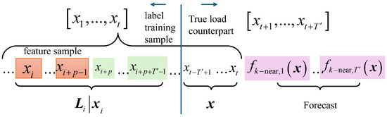
Figure 2.
Data structure definition of fk-near. The structure consists of two parts: the left part contains feature samples used for model training, while the right part represents the short-term load forecasts.
Given a set of historical load power sequences of a certain node, , for instance, starting from any sample, say , continuously intercepting the subsequent samples to form a label training sample, denoted as , where the first q intercepted samples including are called feature samples, denoted as , and the rest sample is called the true load counterpart of the feature sample, denoted as . According to the above definition of label training samples, in theory, no more than label training samples can be extracted from to form a training sample pool, which is . The degree of similarity of label training samples is calibrated by the Euler distance of their feature samples. The closer the value is to 0, the higher the similarity shall be. The k neighbors of a label training sample (or interchangeably, a feature sample) are k numbers of other label training samples (or feature samples) with decreasing similarity.
Referring to the above definition, let represent the number of neighborhood samples associated with the feature sample with the closest Euler distance to the input feature sample , represent the kth closest historical feature sample in the neighborhood of ; note that and represent the true load counterpart of at the j period, and then the load prediction value defined in this article is expressed as [13]:
where
The connotation of (4) is that given a training sample pool, the load forecast is defined to be the weighted sum of true value counterparts of k neighbors of the label training sample with the highest similarity to the feature sample. The similarities are quantified by (5) and (6), respectively. Note that the weights differ from those of [13] in the additional constant of “1”, which is introduced to have the denominator avoiding zero.
When substituting (4)∼(6) into (2) for consecutive load forecasting, forecast errors of individual methods can be monitored based on real-time load. When the error exceeds the prescribed threshold, the newly acquired real-time data can be used to update the label training sample pool. In view of statistical errors of time-series data, this paper uses the Mean Absolute Scaled Error (MASE) as shown in (7):
Based on eMASE, the error criterion for the sample update can be designed, such as eMASE > 15, so that the incremental learning of the feature sample neighborhood is triggered by the error criterion while keeping the volume of the training sample pool unchanged. The specific steps are given below.
First, define a matrix to collect quantitative similarities between all feature samples in the current sample pool, such as
where represents the similarity between feature samples i and j. Then, define a new column vector collecting the similarity between q newly arrived real-time power demands and every feature sample in the current sample pool, denoted by , bring it into (9), and replace in the current sample pool with in the case of :
The following method can be used to minimally update to save the computational overhead based on (9). First, define a vector , and then replace the column and row of with and respectively.
In conclusion, fk-near, developed from [13] in this paper, is intended for complement its father method. The complementation is mainly reflected in the fact that in the case of load sequences with relatively gentle trend changes, both methods utilize a small number of samples in the neighborhood to quickly output prediction (see (4)) through information fusion, maintaining high accuracy and prediction efficiency. On the other hand, when the load sequence mutates, the real-time cumulative prediction error eMASE monitored by fk-near,j, once beyond a threshold, will trigger the replacement and update of neighborhood samples, and compels fk-near,j to use the latest true load values instead of some historical ones long time ago to sustain the feature diversity of the limited training samples. Both embedded methods use real-time data for incremental self-learning. The predicted values of the two methods coincide in the early stage of the training pool, albeit they are diverse over time due to different mechanisms adopted by the two methods to update their training pools, respectively. Based on the short-term lookback performance of the prediction errors of the two methods, the weights of the two methods are consecutively learned via (2) toward the best, as shown later, and the stability of the overall prediction performance can be maintained much better.
4. Self-Healing Strategy of the LVPSA
The self-healing strategy of the LVPSA leverages the load prediction curve from each light-power cabinet’s fog computing unit during the fault repair period, the current status of low-voltage switches, and the estimated fault duration as inputs. These inputs are used to determine the optimal operation strategy for the low-voltage remote-controlled breakers. The specific model is detailed as follows.
The optimization goal is set to minimize the maximum value of the total power loss plus three-phase power imbalance subject to the worst load forecast errors; that is,
where denotes the joint probability distribution of node load demand forecast errors, which falls into the ambiguity set defined by the type-p Wasserstein ball with a radius of ϵ. The nominal distribution involved in defining will be discussed later. represents the node number of the concerned LVPSA, and M represents the penalty coefficient of load shedding. Considering that it is not common for low-voltage power demand to be dispatched smoothly, binary is introduced to indicate the breaker operation of load i at moment t. means that the load is fully supplied, while means disconnecting the load with the grid. is the fog computing node power prediction; that is, , and is the forecast error following . Finally, and and are auxiliary variables introduced to achieve three-phase load balancing at all times.
4.1. Phase Power Balance Constraints
Since a low-voltage user is generally supplied through a single phase, an adjustment of the network switch status may alter load distribution from phase to phase. Three-phase load balance should always be maintained as much as possible. To do this, set constraints
where denotes the phase sending power of the transformer.
4.2. Kirchhoff’s Law
Considering that line parameters in low-voltage station areas are generally difficult to obtain accurately [19], this paper proposes line-parameter-free power flow constraints as shown in (12):
where represents the branch power injected into node j, represents the power-source injected power into node j, and or represent the set of nodes connected by the branches sharing node j as the power receiving or sending end. is the forecast error, which follows the joint probability distribution . The branch power loss needs to be accounted for according to the branch power direction. The specific principle is explained as follows by referring to Figure 3. Suppose that the reference direction of branch power is flowing into node j: if the actual flow direction is consistent with the positive direction (Figure 3a), then according to the assumption ②, the branch loss is calculated as . On the other hand, when the actual flow direction is opposed to the reference (Figure 3b), the power loss is included in , and thus it should be . Therefore, the constraints on can be specifically implemented through the big-M method as follows. First, an auxiliary binary variable is introduced to represent the branch power direction. When it is consistent with the specified reference direction, it is taken as ; otherwise, . The specific expression is given in (13):
where denotes the branch rated capacity. Based on the definition of , the above constraints on can be realized as
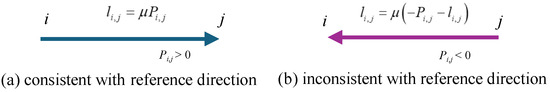
Figure 3.
Branch power loss definition in terms of branch power direction. This definition is used to represent power loss using the big-M method for mixed-integer optimization.
4.3. Switch Status Constraints
Without a loss of generality, represents the operating status of the branch switch between node m and node n at time t. represents the initial state of the switch after fault isolation. The set of nodes either without automatic switches or isolated due to a fault is represented by . Therefore, the switch status constraints should firstly be expressed as
During the fault recovery period, to avoid the risk of secondary power outage to restored users, which could be ascribed to frequent low-voltage switch operations, it is stipulated that “all switches will operate at most once during the fault self-healing period”. Specially,
where denotes the set of complete nodes.
At the same time, in order to always keep the network operating in a radial manner, we can identify all the possible rings. Note that there should be at least three nodes comprising a ring due to the topology feature of the LVPSA under study. Denote the node set belonging to the ith ring by , then
where Card(·) denotes the cardinality operator.
Compared to the virtual line topology constraint method [18], the radiation topology limitation method, which utilizes (18) in conjunction with (16), offers several advantages. It eliminates the need to introduce additional auxiliary variables into the model, reduces the feasible domain of integer variables, and effectively prevents the formation of any loops, regardless of the status of branches and switches. All loops can be pre-identified offline after the installation of facilities such as switches and lines, thereby avoiding the consumption of online computing resources. Furthermore, constraints on the state linkage operation of three-phase switches can be incorporated as needed.
4.4. Boundary Conditions
Equation (19) represents the branch active power and loss constraint restricted by the switch state, and is the constant branch power factor due to assumption ③.
In summary, the switch state reconstruction decision model based on fog computing load prediction proposed in this article consists of (10)∼(19), and the decision variables include , , , , , and . The intact model falls into the “wait-and-see” problem, where the switch states should be decided “here and now”, accounting for the speculated worst effect of the load forecasts. We propose an efficacious method to resolve it in the following section.
4.5. Solution Algorithm
First, we lump all the decision variables in the form of vectors denoted by bold symbols, respectively, and compact the original model (10)∼(19) as a three-stage “Master-Slave” optimization problem below:
Next, let us pick up the thread of defining a necessary nominal distribution for . In order to impose the prior hypotheses as little as possible, the empirical distribution of forecast errors fitting the latest training sample pool of fk-near is employed to play the role of the nominal distribution. By doing this, the nominal distribution varies with the incrementally learning training sample pool. Formally,
where δ(·) is the Dirac function and
To solve the above “Master-Slave” problem, substitute p = 1 into (21) to obtain a type-1 WDRO problem. As per [20] (Theorem 9 therein), the type-1 WDRO on the condition of (22) is equivalent to
Note that (23) is also a two-stage problem with involving integers of and , and we can relax these integers and add constraints [21] like . By doing this, KKT conditions can viably be derived for to convert (23) into a single-layer maximization problem.
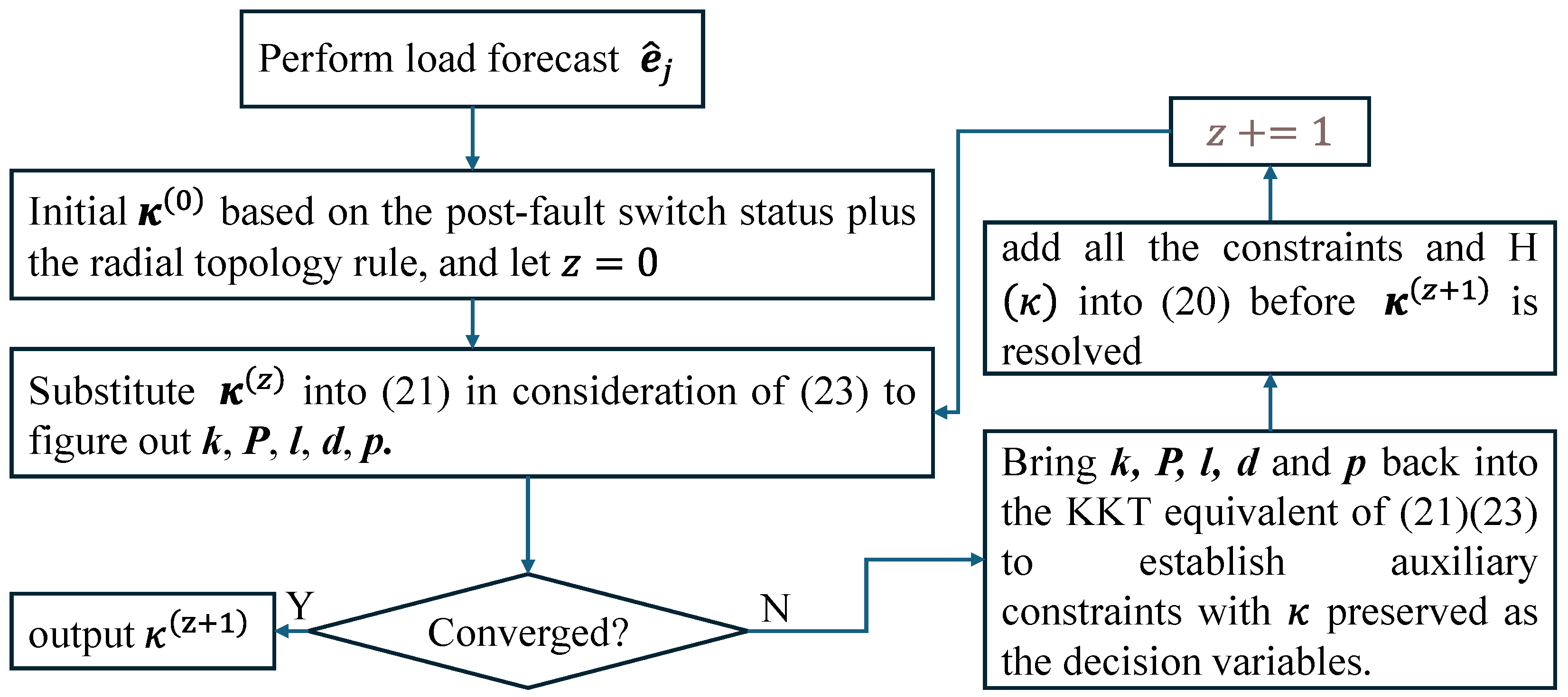
At last, once upon resolving from (23), the column-and-constraint generation algorithm can be employed to add each group of auxiliary variables and constraints with fixed as well as into (20) to proceed with the iteration until convergence criteria, e.g., the gap of the objective value, are satisfied. A relevant flowchart, as shown in Figure 4, outlines the above resolving process.
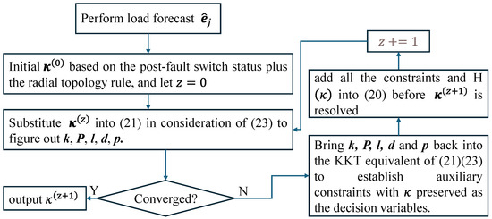
Figure 4.
Flow chart of resolving the proposed self-healing strategy of the LVPSA.
5. Case Studies
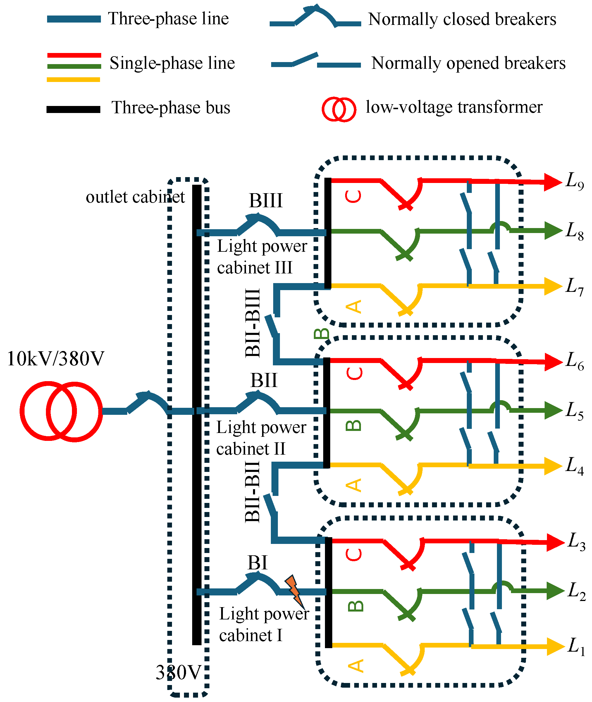
The following case studies consider the addition of phase-to-phase and busbar contact switches in the light-power cabinets downstream of the same power transformer and between cabinets (operation state linked), as shown in Figure 5. The information collection and processing of the nine unbalanced single-phase low-voltage loads L1∼L9 are completed in the fog computing units of their designated light-power cabinets. When the phase voltage is 220 V, and assuming that all single-phase lines are 4 × 150 mm2 copper cables, the branch line loss coefficient can be calculated according to (1) as 0.04. The line length is uniformly set to 3 km, the rated apparent power of the single-phase branch and tie switch is taken to be 0.1 MVA, and the line power factor is taken to be 0.9. The low-voltage distribution transformer and busbar capacity are infinite.
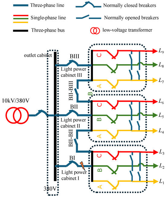
Figure 5.
Simulation test system of an LVPSA.
The low-voltage switch reconstruction and self-healing strategy, based on fog computing load prediction, was developed using Julia (Ver 1.10.4), and Ipopt and Gurobi are called for to solve the weight optimization of (2) and the mixed integer quadratic programming, respectively. The following case studies demonstrate the accuracy of the proposed fog computing load prediction and also discuss the application effect of the LVPSA self-healing strategy.
5.1. Load Forecast Accuracy Tests
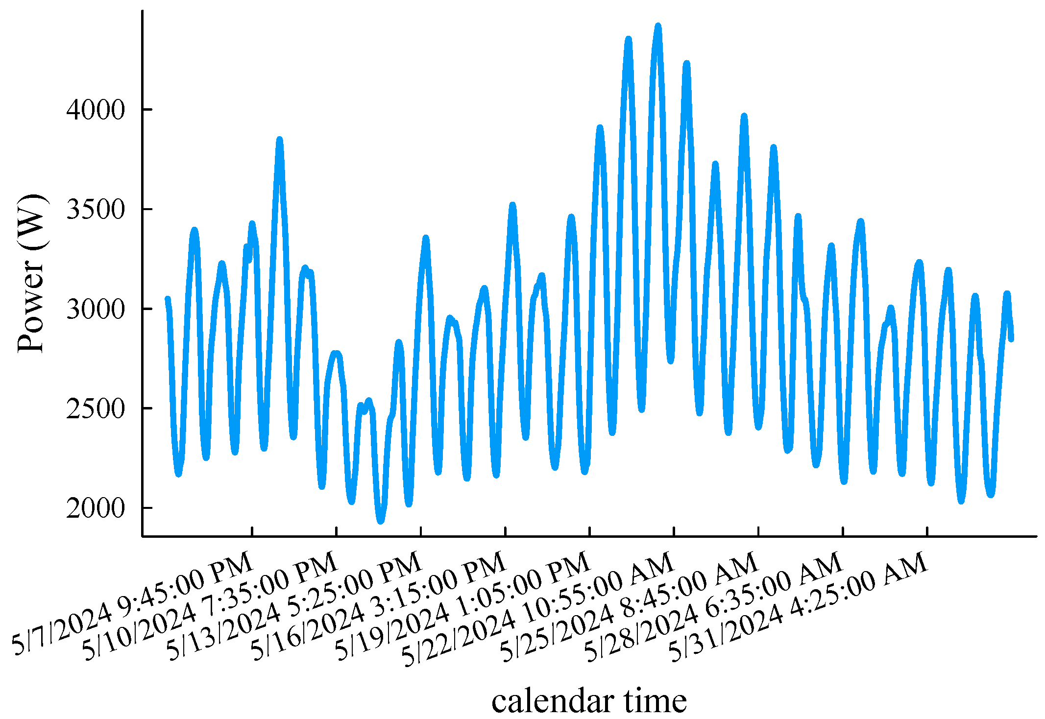
For the load forecast accuracy tests, we used intercepts of the monthly load curve of the 5-minute sampling interval in the “DEQK” area spanning from 12:00 a.m. 5 May 2024 to 1:50 a.m. 3 June 2024 in UTC time from the open-source database [22]. The load records with the same timestamp are averaged, and all the values are uniformly reduced by times to simulate a low-voltage single-phase load (a total of 8375 data points, as shown in Figure 6, which is used to verify the prediction accuracy of the fog computing load prediction method proposed in this article. Taking the lead time of 4 h as an example, that is, , other hyperparameter settings include , , initial weight , and . In order to simplify the explanation, the following algorithms participating in the comparison are named M1, M2, and M1 and M2, respectively. Among them, the M1 method represents the original k-neighborhood prediction method [13], the M2 method is the improved derivative, and M1 and M2 is the fog computing load prediction method.
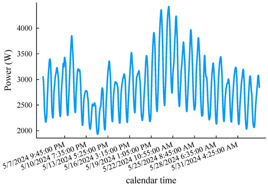
Figure 6.
A 5 min interval load curve emulating monthly low-voltage node power demand.
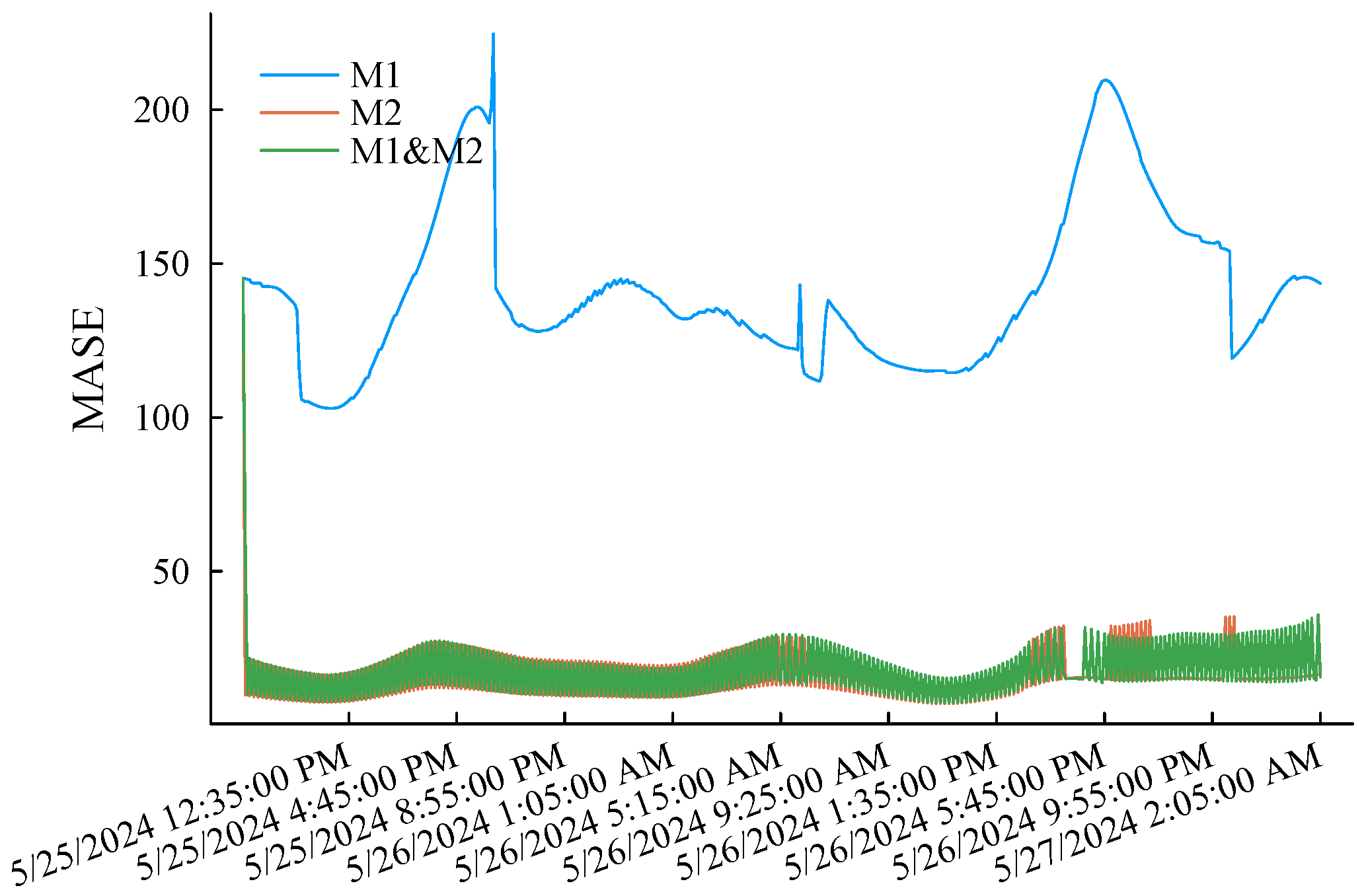
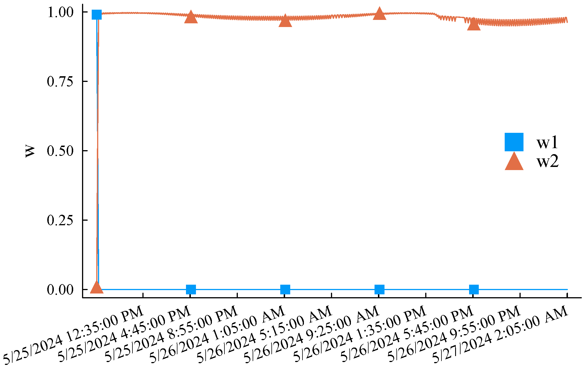
The simulation experiment process is as follows. First, the first of the original low-voltage load curve is selected as the initial training sample. Each experiment uses the latest q samples of the current training pool as the feature sample to predict the load in the subsequent period (a total of 48 prediction points) and compare it with the actual records. After a simulation is completed, the training samples of M1 step forward by one data point, while M2 determines whether it is necessary to update the training sample pool according to the criterion eMASE > 15. M1 and M2 only need to update the weights according to (2). Afterward, the feature sample also steps forward by one data point, and the above simulation experiment process is repeated until the end data of the original load curve are reached. eMASE generated by the three prediction methods during the above complete experimental process is summarized in Figure 7. Taking the prediction error of the M1 as the benchmark reference, it can be clearly observed that the prediction performance of the M2 is much better than the M1 method due to the incremental learning mechanism and dynamically updated training samples. The reason for the significant difference in the prediction error performance between the two methods is that the training samples of the M1 are also dynamic. However, it only intercepts the latest load curve and does not memorize the characteristics of early samples. The M2 also initializes its training sample pool with the load curve but selectively replaces the training samples according to the error threshold, striving to maintain the diversity of limited samples. The M1 and M2 track the error changes in the embedded M1 and M2 through weight optimization. As shown in Figure 8, the methods with smaller historical errors are dynamically given higher weight. The overall error performance is significantly better than M1. The maximum absolute error of single-point prediction is 547.51 W. The last thing to note is that the M1 and M2 maintain the same amount of samples, which is doubled for the proposed method. In this example, , and the memory usage is trivial.
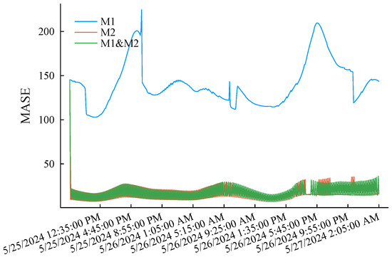
Figure 7.
MASE performance of the three methods applied to the benchmark load curve.
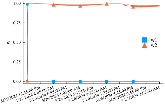
Figure 8.
Adaptive weighting coefficients of the dual embedded incremental learning mechanisms in the proposed approach.
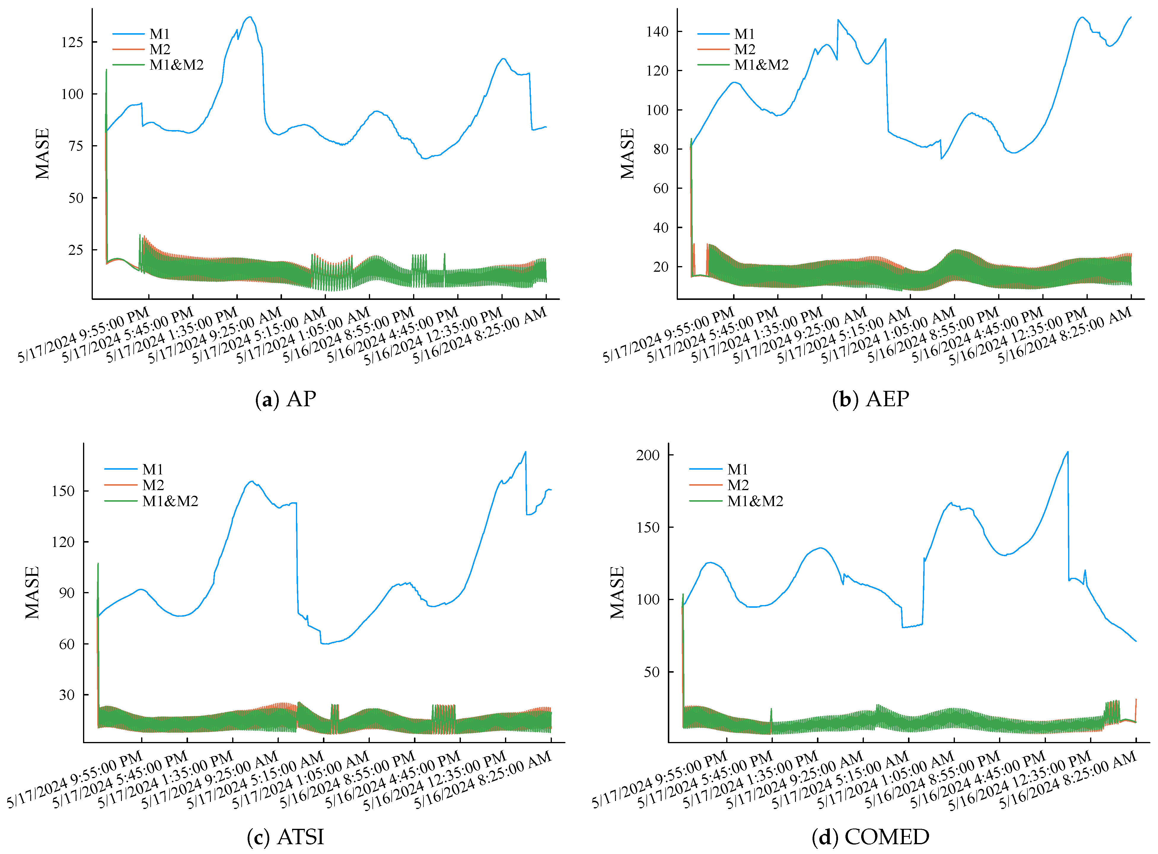
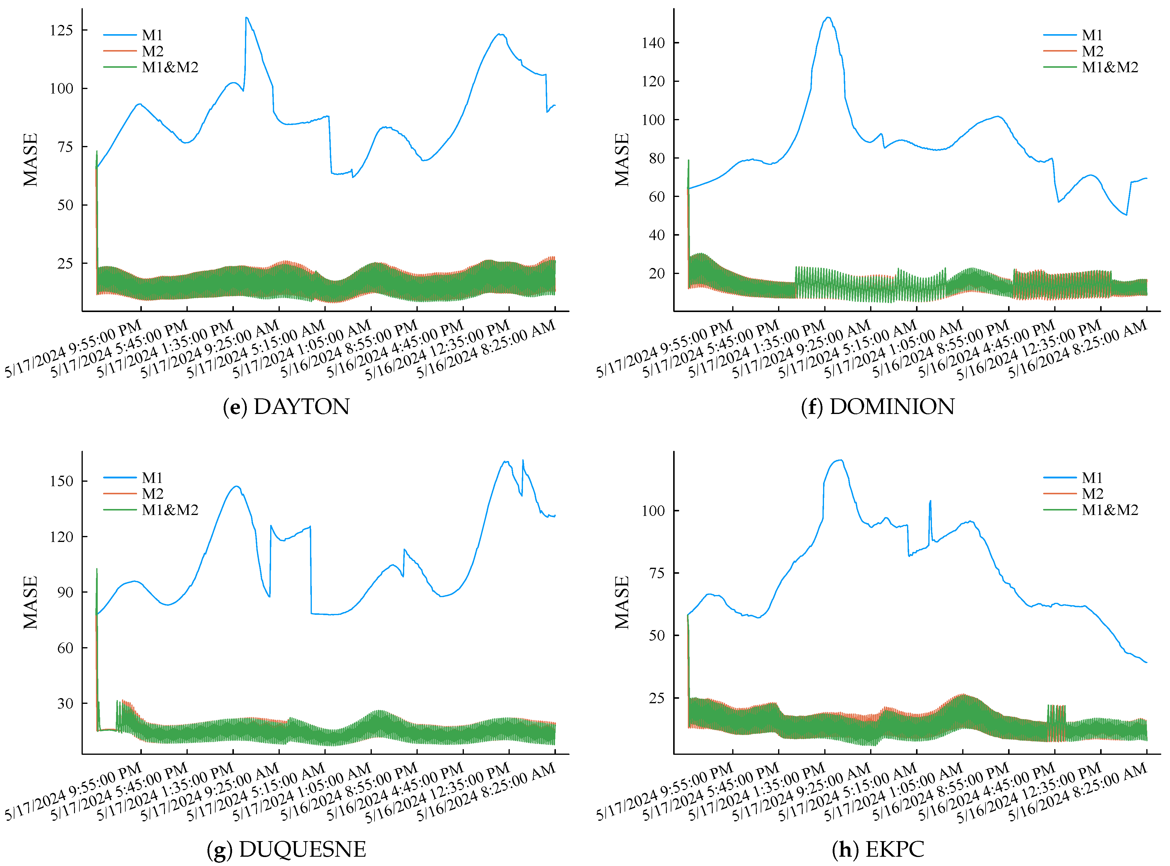
Then, intercept the load curves of eight other regions during the same period and repeat the above simulation experiment process. eMASE of the three methods is summarized in Figure 9. The simulation results further prove the accuracy advantage of the proposed method and its good robustness. The above simulation experiment results show that the fog computing load forecasting method proposed in this article can maintain high load forecasting accuracy through short-memory incremental learning while occupying lower storage and computing resources.
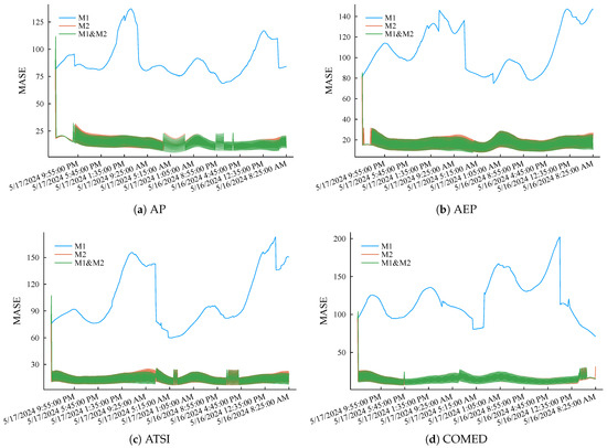
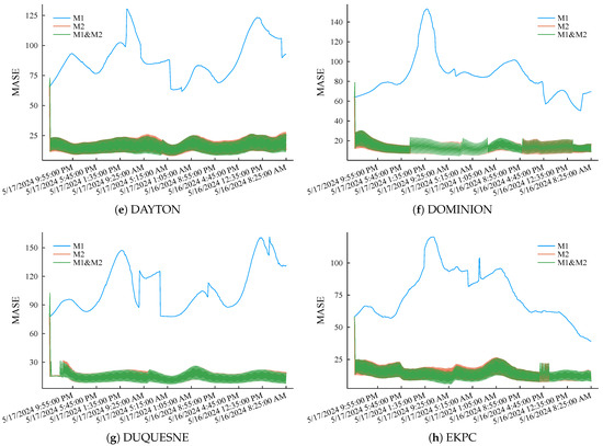
Figure 9.
MASE performance of the three compared methods applied to different regional load curves scaling down to the level of low-voltage nodes.
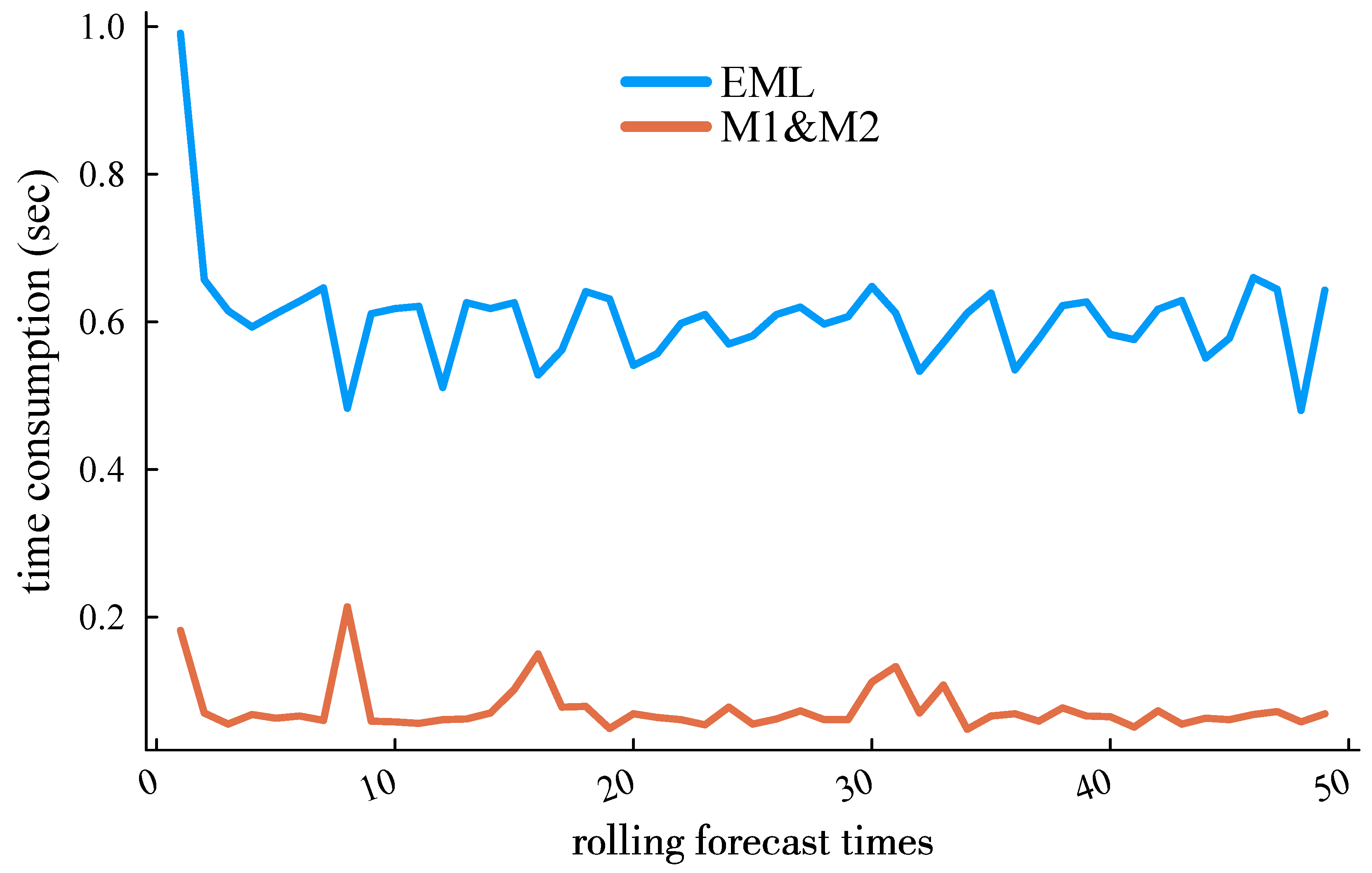
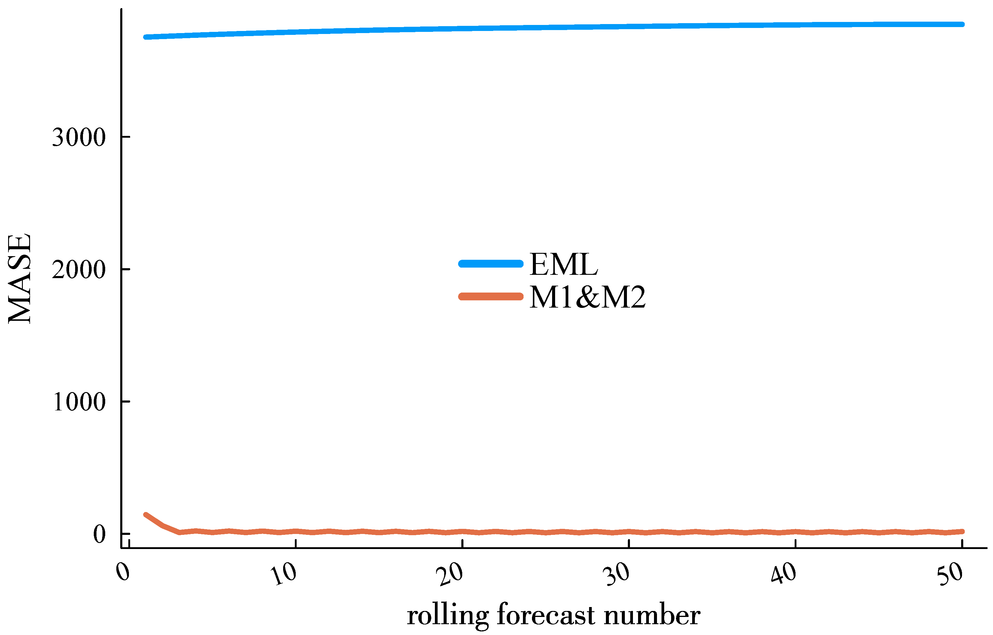
In terms of computational time requirements, mainstream time series load forecasting methods, such as long short-term memory (LSTM) networks and other deep learning approaches, require substantial historical data and significant computing power to achieve algorithmic efficiency. However, due to the storage and floating-point operation limitations of fog computing, a fair comparison among algorithms necessitates the selection of methods with lower computational demands. In addition to the method presented in [13], we included the Extreme Learning Machine (ELM) forecasting method [23] for comparative analysis. The CPU time consumption and Mean Absolute Scaled Error (MASE) of these two methods in rolling ultra-short-term load forecasting are shown in Figure 10 and Figure 11. It is worth noting that Figure 10 reports the total time consumption starting from the initial training sample. The time consumption decreases as the forecasting process progresses, transitioning from the initial model training phase to lighter incremental learning.

Figure 10.
Time consumption of the proposed method and the EML against roll forecast number.
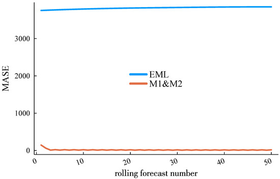
Figure 11.
MASE performance of the proposed method and the EML against roll forecast number.
It is worth noting that Figure 10 reports the total time consumption starting from the initial training sample. The time consumption decreases as the forecasting process progresses, transitioning from the initial model training phase to lighter incremental learning.
It can be observed that the proposed method demonstrates a significantly superior computational efficiency. This advantage arises from two key factors: (1) The comparative ELM method involves extensive matrix computations, particularly in solving the Moore–Penrose generalized inverse matrix, which is a core step in ELM training. (2) During incremental learning, ELM faces challenges in effectively distinguishing temporal features between current and early-stage load data due to its fixed random initialization of input weights. In contrast, the proposed method leverages a lightweight matrix update paradigm (9) and incorporates computationally efficient information fusion techniques, thereby achieving both higher prediction accuracy and reduced computational time.
5.2. Tests on the LVPSA Self-Healing Strategy
The above nine load curves are assumed to correspond to ∼ in Figure 5. This topology contains a total of 32,767 potential loops. It is assumed that the short-circuit fault time is 9:55 p.m. on 26 May 2024, which occurs between the distribution box and “light power cabinet I”. Peak loads of the system for each hour following the fault are 60,598 W, 62,128 W, 64,135 W, and 66,181 W, respectively. All the backup switches situated at the sending ends of the single-phase lines remain open readily before the LVPSA self-healing strategy responds to the fault.
Firstly, to understand a proper model definition of , we arbitrarily select the “DAYTON” load curve () for illustration. The distributions of hourly peak load forecast errors via the M1 and M2, for each sequential 4 hours to the fault time, are plotted in Figure 12. It can be noted that the tails of the error distributions widen with an increasing lead time, and the distribution pattern varies unpredictably. In this regard, the empirical distributions seem to be more rational to govern the forecast error randomness than kinds of parametric distribution functions.
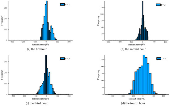
Figure 12.
The hourly peak load forecast error distributions via the M1 and M2 applied to the “DAYTON” load curve (), within the sequential 4 hours to the fault instance.
Secondly, the number of auxiliary variables in (23) will blow up if every error record was used to construct the empirical distributions. Practical application entails a proper number of error samples to balance computation accuracy against speed. Here, the “k-means” method is employed to cluster the original error records of ∼ into 10 categories for every lead time instance, and the centroids are substituted into (23) with . The sequential network configuration schemes are optimized via the proposed LVPSA self-healing strategy and shown in Figure 13. It can be seen from the figure that in general, after the routeway across the transformer and the “light-power cabinet I” is unavailable, the three-phase bus tie switches (BI-BII and BII-BII) between the light-power cabinets and the single-phase switches cooperate with each other to complete the transfer of single-phase loads and maintain network radiation operation with balanced load as much as possible. The obvious topology change happens at , with additional branch links, with the transformer made to be online to balance the more strengthening loading conditions.
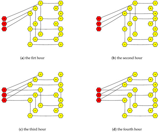
Figure 13.
Optimized sequential configurations via the proposed LVPSA self-healing strategy in response to the fault and short-term load forecasts via fog computing.
6. Conclusions
This paper proposes an LVPSA self-healing strategy cast as a Wasserstein distributionally robust optimization. In terms of LVPSA communication environments, a fog computing load forecasting method is proposed, being essentially a dynamic aggregation of incremental learning models. Practical load samples are employed to demonstrate the efficiency of the time-series forecasts in comparison with the EML algorithm. It is found that the distribution tails of the time-series forecast errors widen as the lead time increases. In this regard, the empirical distributions are employed to govern the load forecast errors in a data-driven manner. As a result, the LVPSA self-healing strategy is formulated by embedding a p-1 WDRO subproblem to account for distribution ambiguity. The intact model is solved using a column-and-constraint generation algorithm based on equivalent KKT conditions for the inner-layer problem of the p-1 WDRO. Case studies were conducted to evaluate the performance of the proposed methods.
Author Contributions
Conceptualization, R.L.; Software, Y.S.; Formal analysis, Y.G.; Resources, H.D., Z.W. and Q.Q.; Data curation, C.Y.; Writing—original draft, W.Y.; Funding acquisition, Y.W. All authors have read and agreed to the published version of the manuscript.
Funding
This research was funded by the Science and Technology Project of State Grid Beijing Electric Power Company, project name: Research and application of precise sensing of low-voltage distribution network status and rapid fault self-healing technology: 52022324000F.
Data Availability Statement
The original contributions presented in this study are included in the article. Further inquiries can be directed to the corresponding author.
Conflicts of Interest
Author Zhiyong Wang was employed by the State Grid Beijing Electric Power Company. Author Qinglei Qin was employed by the State Grid Beijing Yizhuang Electric Power Company. The remaining authors declare that the research was conducted in the absence of any commercial or financial relationships that could be construed as a potential conflict of interest.
Nomenclature
| LVPSA | Passive low-voltage power station area |
| WDRO | Wasserstein distributionally robust optimization |
| Real number set | |
| Number of switches | |
| Number of load points | |
| Branch line loss coefficient | |
| T | Number of historical streaming power demand samples |
| Number of looking-ahead streaming power demand forecasts | |
| e | Load forecasting error |
| Weights of prediction results from different methods | |
| Load forecast result | |
| Operating states of switches | |
| State of Load connection with grid | |
| Branch power flow | |
| Direction of branch power flow | |
| Line power loss |
References
- Sun, L.; Wang, H.; Huang, Z.; Wen, F.; Ding, M. Coordinated Islanding Partition and Scheduling Strategy for Service Restoration of Active Distribution Networks Considering Minimum Sustainable Duration. IEEE Trans. Smart Grid 2024, 15, 5539–5554. [Google Scholar] [CrossRef]
- Poudel, S.; Dubey, A. A two-stage service restoration method for electric power distribution systems. IET Smart Grid 2021, 4, 500–521. [Google Scholar] [CrossRef]
- Chen, Q.; Xu, Z.; Chen, X. Research on the Configuration Scheme and Control Strategy of Automatic Switch in Distribution Station Area. In Proceedings of the 2024 6th International Conference on System Reliability and Safety Engineering (SRSE), Hangzhou, China, 11–14 October 2024; pp. 160–166. [Google Scholar] [CrossRef]
- Magar, A.; Phadke, A. Multi-objective Optimal Placement of Static Transfer Switches in LV Distribution System with PV Penetration. In Proceedings of the 2023 7th International Conference on Computer Applications in Electrical Engineering-Recent Advances (CERA), Roorkee, India, 27–29 October 2023; pp. 1–6. [Google Scholar] [CrossRef]
- Gangwar, P.; Mallick, A.; Chakrabarti, S.; Singh, S.N. Short-Term Forecasting-Based Network Reconfiguration for Unbalanced Distribution Systems With Distributed Generators. IEEE Trans. Ind. Inform. 2020, 16, 4378–4389. [Google Scholar] [CrossRef]
- Liu, Y.; Liang, Z.; Li, X. Enhancing Short-Term Power Load Forecasting for Industrial and Commercial Buildings: A Hybrid Approach Using TimeGAN, CNN, and LSTM. IEEE Open J. Ind. Electron. Soc. 2023, 4, 451–462. [Google Scholar] [CrossRef]
- Liu, F.; Wang, X.; Zhao, T.; Zhang, L.; Jiang, M.; Zhang, F. Novel short-term low-voltage load forecasting method based on residual stacking frequency attention network. Electr. Power Syst. Res. 2024, 233, 110534. [Google Scholar] [CrossRef]
- Liu, Q.; Cao, J.; Zhang, J.; Zhong, Y.; Ba, T.; Zhang, Y. Short-Term Power Load Forecasting in FGSM-Bi-LSTM Networks Based on Empirical Wavelet Transform. IEEE Access 2023, 11, 105057–105068. [Google Scholar] [CrossRef]
- Zhang, X.; Kuenzel, S.; Colombo, N.; Watkins, C. Hybrid Short-term Load Forecasting Method Based on Empirical Wavelet Transform and Bidirectional Long Short-term Memory Neural Networks. J. Mod. Power Syst. Clean Energy 2022, 10, 1216–1228. [Google Scholar] [CrossRef]
- Liu, Y.; Dutta, S.; Kong, A.W.K.; Yeo, C.K. An Image Inpainting Approach to Short-Term Load Forecasting. IEEE Trans. Power Syst. 2023, 38, 177–187. [Google Scholar] [CrossRef]
- Zhou, Y.; Ding, Z.; Wen, Q.; Wang, Y. Robust Load Forecasting Towards Adversarial Attacks via Bayesian Learning. IEEE Trans. Power Syst. 2023, 38, 1445–1459. [Google Scholar] [CrossRef]
- de Moraes Sarmento, E.M.; Ribeiro, I.F.; Marciano, P.R.N.; Neris, Y.G.; de Oliveira Rocha, H.R.; Mota, V.F.S.; da Silva Villaça, R. Forecasting energy power consumption using federated learning in edge computing devices. Internet Things 2024, 25, 101050. [Google Scholar] [CrossRef]
- Melgar-García, L.; Gutiérrez-Avilés, D.; Rubio-Escudero, C.; Troncoso, A. A novel distributed forecasting method based on information fusion and incremental learning for streaming time series. Inf. Fusion 2023, 95, 163–173. [Google Scholar] [CrossRef]
- Massrur, H.R.; Fotuhi-Firuzabad, M.; Dehghanian, P.; Blaabjerg, F. Fog-Based Hierarchical Coordination of Residential Aggregators and Household Demand Response with Power Distribution Grids—Part I: Solution Design. IEEE Trans. Power Syst. 2025, 40, 85–98. [Google Scholar] [CrossRef]
- Massrur, H.R.; Fotuhi-Firuzabad, M.; Dehghanian, P.; Blaabjerg, F. Fog-Based Hierarchical Coordination of Residential Aggregators and Household Demand Response with Power Distribution Grids—Part II: Data Transmission Architecture and Case Studies. IEEE Trans. Power Syst. 2025, 40, 99–112. [Google Scholar] [CrossRef]
- IEEE-P802.11; IEEE Draft Standard for Information Technology—Telecommunications and Information Exchange Between Systems Local and Metropolitan Area Networks—Specific Requirements—Part 11: Wireless LAN Medium Access Control (MAC) and Physical Layer (PHY) Specifications—Amendment 4: Enhancements for Wireless Local Area Network (WLAN) Sensing. IEEE: New York, NY, USA, 2025.
- IEEE 802.15.4; IEEE Standard for Low-Rate Wireless Networks. IEEE: New York, NY, USA, 2024.
- Mahdavi, M.; Alhelou, H.H.; Gopi, P.; Hosseinzadeh, N. Importance of Radiality Constraints Formulation in Reconfiguration Problems. IEEE Syst. J. 2023, 17, 6710–6723. [Google Scholar] [CrossRef]
- Deka, D.; Kekatos, V.; Cavraro, G. Learning Distribution Grid Topologies: A Tutorial. IEEE Trans. Smart Grid 2024, 15, 999–1013. [Google Scholar] [CrossRef]
- Kuhn, D.; Esfahani, P.M.; Nguyen, V.A.; Shafieezadeh-Abadeh, S. Wasserstein Distributionally Robust Optimization: Theory and Applications in Machine Learning. In Operations Research & Management Science in the Age of Analytics; Informs: Catonsville, MD, USA, 2019; Chapter 6; pp. 130–166. [Google Scholar] [CrossRef]
- Medina-González, S.; Papageorgiou, L.G.; Dua, V. A reformulation strategy for mixed-integer linear bi-level programming problems. Comput. Chem. Eng. 2021, 153, 107409. [Google Scholar] [CrossRef]
- Data Miner 2-Five Minute Load Forecast. Available online: https://dataminer2.pjm.com/feed/very_short_load_frcst (accessed on 19 July 2024).
- Chupong, C.; Plangklang, B. Incremental learning model for load forecasting without training sample. Comput. Mater. Contin. 2022, 72, 5415–5427. [Google Scholar] [CrossRef]


Disclaimer/Publisher’s Note: The statements, opinions and data contained in all publications are solely those of the individual author(s) and contributor(s) and not of MDPI and/or the editor(s). MDPI and/or the editor(s) disclaim responsibility for any injury to people or property resulting from any ideas, methods, instructions or products referred to in the content. |
© 2025 by the authors. Licensee MDPI, Basel, Switzerland. This article is an open access article distributed under the terms and conditions of the Creative Commons Attribution (CC BY) license (https://creativecommons.org/licenses/by/4.0/).