Dispatch for the Industrial Micro-Grid with an Integrated Photovoltaic-Gas-Manufacturing Facility System Considering Carbon Emissions and Operation Costs

Abstract

In this paper, the dispatch for the industrial micro-grid with an integrated photovoltaic-gas-manufacturing facility system considering carbon emissions and operation costs is investigated. Two kinds of energy, electricity and natural gas, are contained in the integer energy system, in which the electricity mainly comes from the PV panels and the utility electricity network, and the natural gas mainly comes from the utility gas network. In addition, electricity and natural gas can be converted into each other. Four kinds of loads, electricity load, gas load, heating load and cooling load, need to be satisfied, in which the electricity load can be divided into fixed load and flexible load. The flexible load comes from the scheduling for manufacturing facilities, and the scheduling of manufacturing facilities is modeled as a kind of deferable load to be integrated into the energy system. Moreover, daily operation costs and carbon emissions are considered in the decision, and the deviation preference strategy is used to solve this multi-objective optimization problem. Finally, a case study with a lithium-ion battery assembly system is proposed. According to the results, it can be found that the proposed model can help managers realize effective scheduling of the industrial micro-grid.

1. Introduction

Economic development has led to the sustained growth of electricity demand. Energy consumption is expected to grow by $44\%$ from 2006 to 2030 [1]. The dependence of the traditional power grid on fossil-centralized power generation is unsustainable. On the one hand, fossils are non-renewable energy sources. On the other hand, fossil fuel burning produces a large amount of carbon dioxide, causing a serious problem with the greenhouse effect [2]. According to statistics, energy-related carbon dioxide emissions account for two-thirds of global greenhouse gas emissions.

This situation promotes the transformation from the traditional grid to the smart grid. Compared with traditional fossil energy, renewable energy has the advantages of rich resources, easy access, a environment-friendly power generation process, a low power generation cost and so on [3]. Promoting the development of renewable energy can promote the transformation of the power grid and accelerate the process of economic development at the same time [4]. However, the uncertainty of renewable energy generation poses a challenge to the reliability and stability of the power grid [5].

In addition, the traditional cogeneration operation mode seriously limits the flexibility and economy of the system operation [6]. According to the development trend of renewable energy, integrated energy systems (IESs) have broken the barrier of physical isolation between traditional energy systems and realized the linkage between independent energy subsystems [7,8]. In an integrated energy system, the gap between the supply side and the demand side of energy can be narrowed by energy storage. At the same time, integrated energy systems can simultaneously dispatch users’ power, gas, heating, cooling and other types of energy systems to meet their different needs [9]. It is feasible to generate greater cost reductions for energy users by taking into account the modeling and optimization of IESs for energy carriers such as electricity, heating, cooling and natural gas. As a result, having an effective and ideal scheduling plan is crucial.

At present, there are some related studies on IES scheduling. A new type of energy unit, We-Energy, is suggested with full duplex and multi-energy carrier coupling interactions. An IES with combined thermal and electricity supply is expanded with a concentrated solar power plant [10]. Additionally, a typical system structure architecture is created by combining energy conversion equipment made up of an electric heater, an energy storage device and a wind power plant [11]. To obtain the IES scheduling result, a related two-stage multi-objective optimal scheduling approach is proposed [12]. In [13], a novel bi-level optimal dispatching model for a community integrated energy system with an electric vehicle charging station in multi-stakeholder situations is established. A time-coordinated operational strategy for IES scheduling is suggested, and the energy recovery equipment in coal mines is simulated [14]. And the game strategy is used to investigate the isolated island electric–gas deeply coupled energy network in [15]. Furthermore, the optimization scheduling of a wind–photovoltaic–gas–electric vehicle community integrated energy system considering uncertainty and carbon emissions reduction is investigated in [16,17,18]. The operational optimization of regional integrated energy systems with heat pumps and hydrogen renewable energy under integrated demand response is investigated [19]. Yang et al. propose a multi-energy pricing strategy for port integrated energy systems based on a contract mechanism [20]. An elite genetic algorithm-based self-sufficient energy management system for an integrated energy station is designed in [21]. A comprehensive resilience assessment framework is designed to investigate the influence of gas–thermal inertia and power–gas–heat interdependency on IES resilience performance in scheduling [22].

However, there is little literature on the scheduling problem of IESs in factories. The industrial sector, as the largest consumer of electricity, is the sector most affected by the transformation of the power structure compared with the residential and commercial sectors. Therefore, it is of great significance to promote the transformation of the power system in the industrial sector [23]. However, the time–space coupling in the industrial production process, such as the flow of production materials, free space in the buffer and continuity between industrial processes, makes it difficult for factories to respond to the intermittent nature of renewable energy power generation [24]. There is a lot of literature modeling the factory manufacturing process [25]. A state–task network-based industrial process model was proposed and used to resolve the price-driven day-ahead scheduling problem in oxygen generation facilities [26]. However, the proposed model ignores the machine operating sequence. Furthermore, a discrete manufacturing model was designed and applied for real-time load reduction bids [27]. Meanwhile, the discrete manufacturing model has been further improved in [28]. But there are certain issues with the most recent discrete manufacturing assembly model in terms of applicability, such as buffer blockages, excess machine workload and inadequate material supply. More constraints between adjacent machines and buffers were added such that the discrete model was more realistic [29]. In addition, a newly discrete manufacturing assembly model was proposed by regarding the production line as a kind of deferrable load, which simplifies the scheduling decision-making process [30]. The newly simplified model was used in the energy trading problem, while considering only a single energy source.

Motivated by these discussions, this paper focuses on the dispatch of an integrated photovoltaic-gas-manufacturing facility system considering carbon emissions and operation costs. The contributions are explained in further detail as follows:

(1) Differently from previous references on IES scheduling, the diversity of equipment types in IESs is fully considered in this paper, including the conventional gas turbine (CGT), power-to-gas (P2G), absorption chiller (AC), waste heat boiler (WHB), electrical boiler (EB), electrical cooler (EC), gas boiler (GB), battery energy storage system (BESS), PV panels and manufacturing facilities.

(2) Differently from previous references on manufacturing assembly systems, the production line in the manufacturing assembly system is regarded as a kind of deferrable load, and the manufacturing assembly system is integrated into the IES. This provides a strategy for assembly factories to adjust equipment according to different production tasks.

(3) The economy and environment are considered at the same time in this paper, and the deviation preference optimization strategy is proposed for solving the multi-objective problem, in which the deviation preference of the decision-maker will decide the weights of the economy and environment.

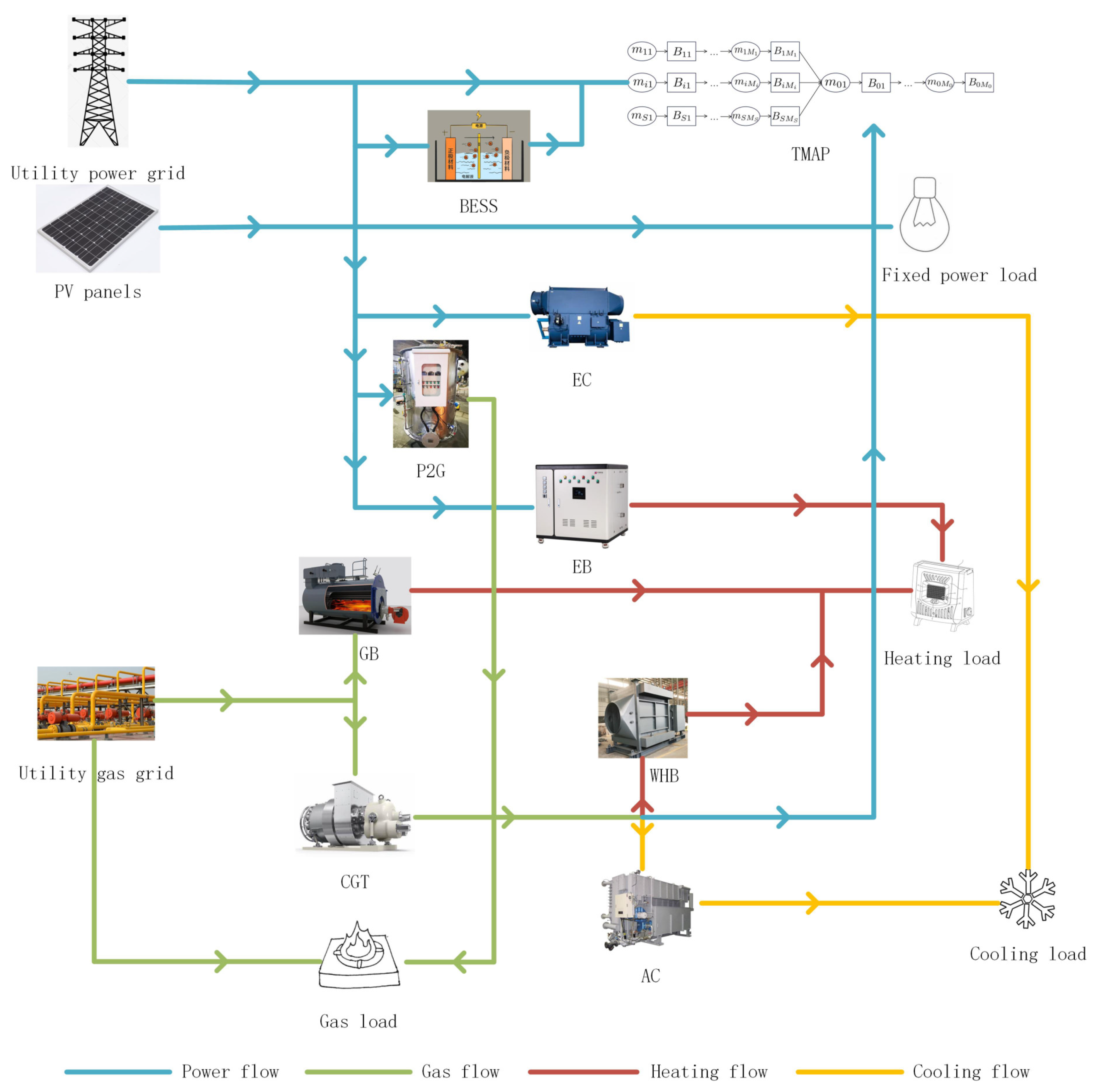
2. Problem Formulation

In this paper, the dispatch of an integrated energy system is considered, and the schematic diagram is shown in Figure 1. Two kinds of energy are supplied to the integrated energy system. The first is electricity, which is supplied by the utility power network and the PV panels. The second is natural gas, which is supplied by the utility gas network. Accordingly, there are four kinds of loads that need to be met, i.e., the electricity load, the gas load, the heating load and the cooling load. The electricity load can be divided into the fixed electricity load and deferrable load, in which the fixed electricity load contains lighting equipment, monitoring equipment, etc., and the deferrable load is composed of the facilities of the typical manufacturing assembly process. The other three types of loads are fixed, in which the heating load and cooling load depend mainly on the outdoor temperature. In addition, the conventional gas turbine (CGT) and power-to-gas (P2G) are added for the conversion between electricity and natural gas. The absorption chiller (AC) and waste heat boiler (WHB) are added to absorb waste heat caused by the CGT. The electrical boiler (EB), electrical cooler (EC) and gas boiler (GB) are added to guarantee the satisfaction of the heating and cooling loads. The scheduling time is equally divided into T time periods, and each time period lasts $▵T$. Let $t\in \{1,2,...,T\}$ indicate the time periods. The mathematical modeling of each component is discussed as follows.

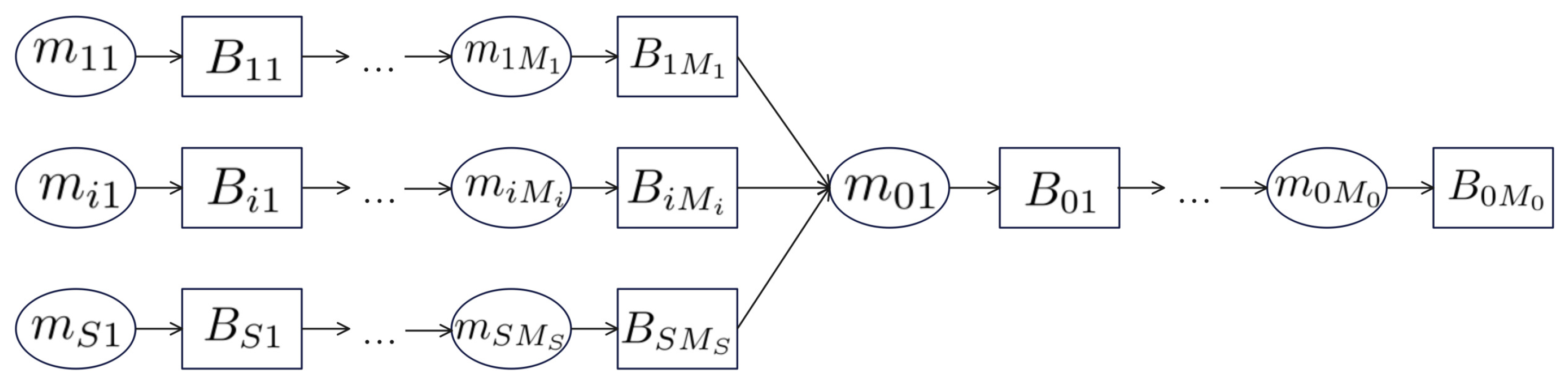
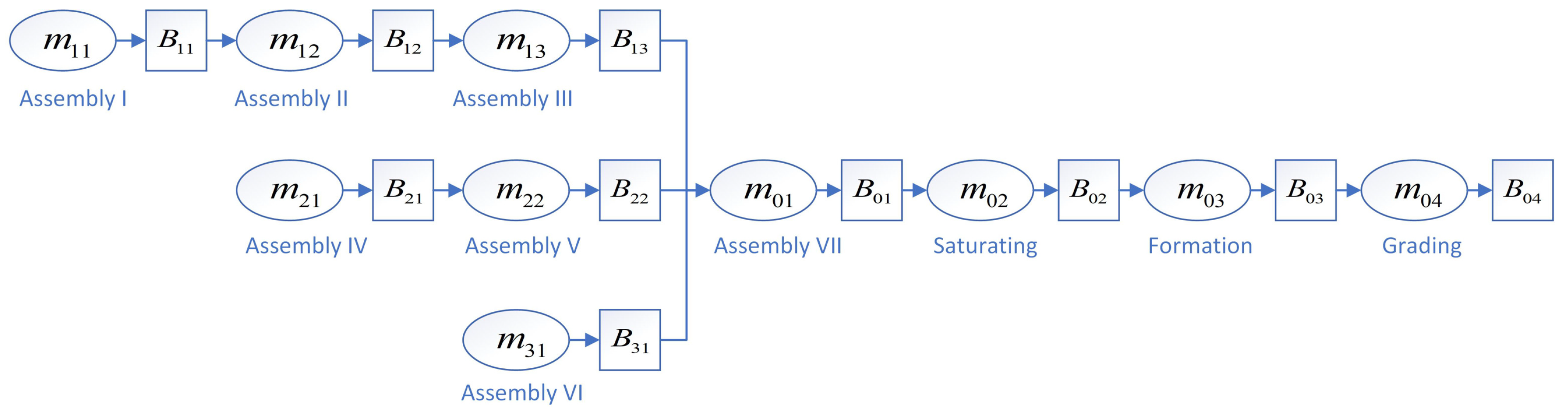
2.1. Typical Manufacturing Assembly Process

The typical manufacturing assembly process is the main part of the factory, in which the manufacturing facilities can be flexibly adjusted to respond to renewable energy generation. However, the traditional model for the typical manufacturing assembly process is too discrete. In this section, the typical manufacturing assembly process is modeled in terms of the production line. As shown in Figure 2, there are S component production lines and an assembly line, and each line has $M_i$ manufacturing facilities. Let the first subscript i represents the production line, where $i\in \{1,2,...,S\}$ indicates the component production lines and $i=0$ indicates the assembly line. In addition, the second subscript j represents the manufacturing facilities. Some assumptions are given firstly to integrate the typical manufacturing assembly process into the overall energy system.

Assumption 1:

Every facility has the same productivity, yet each facility has a single consumption rate.

Assumption 2:

The material supply of the first facility to the component production line is always sufficient.

Assumption 3:

The assembly factory has a fixed daily production task, which is symbolized as D.

Assumption 4:

The facility cannot be stopped once it has started operating until its daily production task has been finished.

Assumption 5:

Taking the production line as the unit, after the first facilities of each production line start to run, the follow-up facilities need to run in turn according to the operation conditions established in advance.

Based on the above assumptions, the working hours of machines are fixed and the same: $l:=\lceil D/n\rceil$, where n represents the productivity and $\lceil ·\rceil$ denotes rounding up. Let $u_{ij}$ symbolize the rated power of machine $m_{ij}$. If the first facility of the production line i starts to run at the beginning of the time interval $t_i$, the demanded powers of the line during different time intervals are shown in

Table 1. The consumed power of line i when $l>M_i$.

Time Step t	Consumed Power
$t_i$	$u_{i1}$
$t_i+1$	$u_{i1}+u_{i2}$
⋯	⋯
$t_i+M_i-1$	$u_{i1}+u_{i2}+\cdots +u_{i{M}_i}$
$t_i+M_i$	$u_{i1}+u_{i2}+\cdots +u_{i{M}_i}$
⋯	⋯
$t_i+l-1$	$u_{i1}+u_{i2}+\cdots +u_{i{M}_i}$
$t_i+l$	$u_{i2}+u_{i3}+\cdots +u_{i{M}_i}$
⋯	⋯
$t_i+l+M_i-2$	$u_{i{M}_i}$

and

Table 2. The consumed power of line i when $l<M_i$.

Time Step t	Consumed Power
$t_i$	$u_{i1}$
$t_i+1$	$u_{i1}+u_{i2}$
⋯	⋯
$t_i+l-1$	$u_{i1}+u_{i2}+\cdots +u_{i,l}$
$t_i+l$	$u_{i2}+u_{i3}+\cdots +u_{i,l+1}$
⋯	⋯
$t_i+M_i-1$	$u_{i,M_i-l+1}+\cdots +u_{i{M}_i}$
⋯	⋯
$t_i+l+M_i-2$	$u_{i{M}_i}$

. And the demanded powers in the tables are zeros.

In this situation, every production line can be thought of as a deferable load; that is, the machine $m_{i1}$ turning on can be thought of as a signal that the deferable load has been placed. A binary vector ${\mathit{s}}_i={[s_{i,1},s_{i,2},\cdots ,s_{i,T}]}^{\prime }$ is added as a control switch for line i. $s_{i,t}$ is valued as 1 if machine $m_{i1}$ turns on during time period t, and 0 otherwise. Every production line can be operated once, which can be described as follows:

$$sum\left({\mathit{s}}_i\right)=1,\forall i\in \mathcal{I},$$

(1)

where $sum(·)$ represents the sum of all elements of the vector. Meanwhile, the constraints of time coupling between CPLs and the assembly line can be described as follows:

$$\mathfrak{h}({\mathit{s}}_0-{\mathit{s}}_i)\ge M_i,\forall i\in \mathcal{I}\backslash \left\{0\right\},$$

(2)

where $\mathfrak{h}=[1,2,...,T]$ is the given row vector. Furthermore, $m_{0M_0}$ has to perform l time steps to ensure the completion of the daily task, which indicates that the latest permissible start time for the assembly line is $T-M_0-l+2$. Hence, the following constraint should be satisfied:

$$\mathfrak{h}·{\mathit{s}}_0\le T-M_0-l+2.$$

(3)

Let ${\mathit{c}}_{i,1}={[c_{i,1},c_{i,2},\cdots ,c_{i,T}]}^{\prime }$ represent the power consumption of line i if $s_{i,1}=1$, which can be calculated from Table 1 and Table 2; ${\mathit{P}}_i=[P_{i,1},P_{i,2},\cdots ,P_{i,T}]$ denotes the final power consumption result after scheduling. Then,

$${\mathit{P}}_i={\mathit{C}}_i{\mathit{s}}_i,\forall i\in \mathcal{I},$$

(4)

where

$$\begin{array}{ccc}\hfill {\mathit{C}}_i& =& [{\mathit{c}}_{i,1},{\mathit{c}}_{i,2},\cdots ,{\mathit{c}}_{i,T}]\hfill \\ & =& \left[\begin{array}{cccc}{c}_{i,1}& c_{i,T}& \cdots & c_{i,2}\\ c_{i,2}& c_{i,1}& \cdots & c_{i,3}\\ \cdots & \cdots & \cdots & \cdots \\ c_{i,T}& c_{i,T-1}& \cdots & c_{i,1}\end{array}\right].\hfill \end{array}$$

(5)

2.2. Battery Energy Storage System

The battery energy storage system is used in two situations. The BESS charges when there is too much PV generation, while discharging when PV generation is insufficient. Since the integrated energy system is connected with the utility power network, the charging and discharging of the BESS occur if and only if the difference between the buying price from the network and the selling price to the network is greater than the degradation cost caused by BESS operation. Assume that the degradation cost is linearly related to the charging/discharging power. Let $c_B$ be the cost parameter and $P_{dis,t}^{BESS}$ and $P_{cha,t}^{BESS}$ the discharging and charging power of the BESS during time period t. The degradation cost can be represented as follows:

$$f_{B,t}=c_B(P_{dis,t}^{BESS}+P_{cha,t}^{BESS})▵T.$$

Generally, charging and discharging cannot occur simultaneously. Therefore, the binary variable ${\eta }_{e,t}^{BESS}$ is added, and the maximum charging and discharging limits, $P_{dis,max}^{BESS}$ and $P_{cha,max}^{BESS}$, are represented as follows:

$$\begin{array}{c}\hfill 0\le P_{dis,t}^{BESS}\le {\eta }_{e,t}^{BESS}{P}_{dis,max}^{BESS},\forall t\in \left[T\right],\end{array}$$

(6)

$$\begin{array}{c}\hfill 0\le P_{cha,t}^{BESS}\le (1-{\eta }_{e,t}^{BESS})P_{cha,max}^{BESS},\forall t\in \left[T\right].\end{array}$$

(7)

When the BESS is discharging, ${\eta }_{e,t}^{BESS}:=1$ and constraint (7) degenerates to $P_{cha,t}^{BESS}=0$. When the BESS is charging, ${\eta }_{e,t}^{BESS}:=0$ and constraint (6) degenerates to $P_{dis,t}^{BESS}=0$. In addition, the state of charge (SoC) should be within a certain range. Otherwise, it will affect the life of the BESS. This limit can be represented by the following mathematical formulation:

$$So{C}_{min}\le So{C}_t\le So{C}_{max},$$

(8)

where $So{C}_{t+1}=So{C}_t+{\displaystyle \frac{1}{E_{B,r}}}(P_{cha,t}^{BESS}{\beta }_{B,c}-P_{dis,t}^{BESS}/{\beta }_{B,d})▵T$; $E_{B,r}$ symbolizes the rated capacity; and ${\beta }_{B,c}$ and ${\beta }_{B,d}$ denote the charging and discharging efficiency coefficients.

2.3. Photovoltaic Power Generation

As a kind of renewable energy, the generation of PV is uncertain, and can be influenced by solar radiation, temperature, humidity, wind speed, etc. For day-ahead scheduling, PV generation needs to be predicted according to historical data and weather forecasts, which are always unmatched with the actual generation. In this regard, the Wasserstein-based metric distributionally robust chance constraints are used to guarantee that the power demand can be satisfied within probability $1-\epsilon$:

$$\underset{{\mathbb{P}}_t\in {\mathfrak{F}}_t}{inf}{\mathbb{P}}_t(-P_{\underline{r},t}\le {\xi }_t\le P_{\overline{r},t})\ge 1-\epsilon ,\forall t\in \left[T\right],$$

where ${\xi }_t$ represents the error between the predictive and actual PV generation, i.e., ${\xi }_t={\widehat{P}}_{e,t}^{PV}-P_{e,t}^{PV}$, and ${\xi }_t$ is a random variable; ${\widehat{P}}_{e,t}^{PV}$ is the predictive PV generation according to the history data-set; $P_{e,t}^{PV}$ is the actual PV generation in real time; $\mathfrak{F}$ is the Wasserstein ambiguity set constructed by the history data-set with radius $\theta$; and ${\mathbb{P}}_t$ symbolizes the worst-case probability distribution. The deficiency/excess of PV generation is dealt with by the reserve capacity of the conventional generator for real-time operation. This joint distributionally robust chance constraint (DRCC) ensures that the underlying constraint is satisfied, with the minimum probability of $1-\epsilon$ under the worst-case distribution.

According to [30], the joint DRCC can be approximated as follows:

$$\left\{\begin{array}{c}\theta -\epsilon {\gamma }_t\le {\displaystyle \frac{1}{N}}{\sum }_{n=1}^N{\kappa }_{n,t},\hfill \\ {\kappa }_{n,t}+{\gamma }_t\le {\widehat{\xi }}_t^n+P_{\underline{r},t},\forall n\in \mathcal{N},\hfill \\ {\kappa }_{n,t}+{\gamma }_t\le P_{\overline{r},t}-{\widehat{\xi }}_t^n,\forall n\in \mathcal{N},\hfill \\ {\kappa }_{n,t}\le 0,\forall n\in \mathcal{N},\hfill \\ {\gamma }_t\ge 0.\hfill \end{array}\right.$$

(9)

Furthermore, the battery energy storage system is used to cope with renewable power deficits (excess) in real-time operation. Hence, the following limits should be considered:

$$P_{\underline{r},t}+P_{cha,t}\le (So{C}_{max}-So{C}_{t-1})·E_{B,r}/▵T,$$

(10)

$$P_{\overline{r},t}+P_{dis,t}\le (So{C}_{t-1}-So{C}_{min})·E_{B,r}/▵T,$$

(11)

$$0\le P_{\underline{r},t},$$

(12)

$$0\le P_{\overline{r},t},$$

(13)

in which the first constrain indicates the charging energy during time interval t, which is decided by the sum of the downward reserve and charging power, and cannot cause the state of charge to exceed the maximum limit; the second constrain indicates the discharging energy during time interval t, which is the sum of the downward reserve and charging power, and cannot cause the state of charge to be below the maximum limit; and the last two constraints mean that the reserve power cannot be negative.

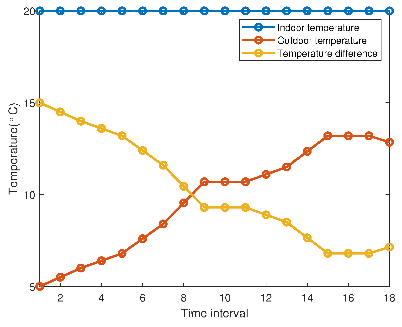
2.4. Heating Load and Cooling Load

In addition to the fixed heating and cooling loads, the outdoor temperature will also have an impact on the heating and cooling loads of the factory. Let $P_{h,t}^{FL}$ and $P_{c,t}^{FL}$ symbolize the fixed heating and cooling loads, which are not affected by outdoor temperature. The additional heating and cooling loads depend on the difference between the set indoor temperature and the real-time outdoor temperature. ${\eta }_{tem,t}$ is introduced to indicate whether the heating or cooling load is needed during the time period t. If ${\eta }_{tem,t}:=1$, the outdoor temperature is lower than the set indoor temperature, and the heating load is needed. Otherwise, ${\eta }_{tem,t}:=0$. It should be noted that ${\eta }_{tem,t}$ is not a variable that should be determined by optimization. On the contrary, ${\eta }_{tem,t}$ is a definite value if the set indoor temperature and the outdoor temperature are determined. Therefore, the values of the flexible heating load and flexible cooling load can be calculated as follows:

$$P_{h,t}^L={\eta }_{tem,t}\ast {\displaystyle \frac{T_t^{in}-T_t^{out}+\frac{K\ast F}{C_{air}{\rho }_{air}V}\ast ▵T\ast (T_{t-1}^{in}-T_t^{out})}{\frac{1}{K\ast F}+\frac{1}{C_{air}{\rho }_{air}V}\ast ▵T}},$$

(14)

$$P_{c,t}^L=(1-{\eta }_{tem,t})\ast {\displaystyle \frac{T_t^{out}-T_t^{in}+\frac{K\ast F}{C_{air}{\rho }_{air}V}\ast ▵T\ast (T_{t-1}^{out}-T_t^{in})}{\frac{1}{K\ast F}+\frac{1}{C_{air}{\rho }_{air}V}\ast ▵T}},$$

(15)

where $P_{h,t}^L$ symbolizes the flexible heating load during the time period t; $P_{c,t}^L$ symbolizes the flexible cooling load during the time period t; $T_t^{in}$ is the indoor temperature during the time period t; $T_t^{out}$ is the outdoor temperature during the time period t; K represent the comprehensive heat transfer factor; F denotes the building surface area; $C_{air}$ is the heat capacity of indoor air; ${\rho }_{air}$ is the density of the indoor air; and V is the building volume.

2.5. Conventional Gas Turbine

The conventional gas turbine (CGT) and power-to-gas (P2G) are added for the conversion between electricity and natural gas in the energy system. It is an example of a common decentralized system representation, where the CGT is always combined with the WHB and AC to form a combined cooling heating and power system. On the one hand, the CGT is used to consume gas to generate electricity, and the relationship between the consumed natural gas $P_{g,t}^{CGT}$ and the generated electricity $P_{e,t}^{CGT}$ is shown below:

$$P_{e,t}^{CGT}={\displaystyle \frac{P_{g,t}^{CGT}\ast HHV\ast {\beta }_{CGT}}{▵T}},$$

(16)

where $HHV$ denotes the high heating value of natural gas; ${\beta }_{CGT}$ represents the power generation efficiency of the CGT.

On the other hand, waste heat will be generated during the conversion process, and the relationship between the consumed natural gas $P_{g,t}^{CGT}$ and the waste heat $P_{WH,t}$ is shown below:

$$\begin{array}{c}\hfill P_{WH,t}=P_{g,t}^{CGT}\ast HHV\ast {\beta }_{WH},\end{array}$$

(17)

where ${\beta }_{WH}$ is the heat loss coefficient. The WHB and AC can both use waste heat. The AC uses it to supply cold energy, whereas the WHB uses it to supply thermal energy. Different from existing references, incomplete utilization of waste heat is allowed in this paper, and the relationship between the cold energy $P_{c,t}^{AC}$, the thermal energy $P_{h,t}^{WHB}$ and the waste heat is shown below:

$$\begin{array}{c}\hfill P_{WH,t}\ge P_{c,t}^{AC}/{\beta }_{AC}+P_{h,t}^{WHB}/{\beta }_{WHB},\end{array}$$

(18)

where ${\beta }_{AC}$ is the performance coefficient of $AC$; ${\beta }_{WHB}$ is the thermal efficiency. In addition, the input natural gas of the CGT, the output cold energy and thermal energy are limited by the equipment. The constraints of the CGT, AC and WHB are formulated as follows:

$$0\le P_{g,t}^{CGT}\le P_{max}^{CGT},$$

(19)

$$0\le P_{g,t}^{AC}\le P_{max}^{AC},$$

(20)

$$0\le P_{g,t}^{WHB}\le P_{max}^{WHB},$$

(21)

where $P_{max}^{CGT}$, $P_{max}^{AC}$ and $P_{max}^{WHB}$ denote the maximum value of the CGT, AC and WHB, respectively.

2.6. Power to Gas

P2G, as opposed to the CGT, generates natural gas through two reaction stages using electricity. First, an electrolyzer uses $H_{2}0$ to electrolyze $H_2$ and $O_2$. Next, the Sabatier reaction uses $H_2$ and $C{O}_2$ to generate $C{H}_4$. The natural gas produced by P2G is proportion to the input power $P_{e,t}^{P2G}$ and conversion efficiency ${\beta }_{P2G}$:

$$P_{g,t}^{P2G}={\displaystyle \frac{P_{e,t}^{P2G}\ast {\beta }_{P2G}\ast ▵T}{HHV}}.$$

(22)

The input power is limited by the maximum input power $P_{max}^{P2G}$ of the equipment:

$$0\le P_{e,t}^{P2G}\le P_{max}^{P2G}.$$

(23)

2.7. Electrical Boiler

Since the thermal energy generated by the WHB is limited by the CGT, the electrical boiler (EB) is added to consume electricity to generate thermal energy. The relationship between the input power $P_{e,t}^{EB}$ and the output thermal energy $P_{h,t}^{EB}$ is formulated as follows:

$$P_{h,t}^{EB}=P_{e,t}^{EB}\ast {\beta }_{EB}\ast ▵T,$$

(24)

where ${\beta }_{EB}$ is the conversion efficiency. The input power is limited by the maximum power of equipment $P_{max}^{EB}$, which is described as follows:

$$0\le P_{e,t}^{EB}\le P_{max}^{EB}.$$

(25)

2.8. Electrical Cooler

Since the cold energy generated by the AC is limited by the CGT, the electrical cooler (EC) is added to consume electricity to generate cold energy. The relationship between the input power $P_{e,t}^{EC}$ and the output cold energy $P_{c,t}^{EC}$ is formulated as follows:

$$P_{c,t}^{EC}=P_{e,t}^{EC}\ast {\beta }_{EC}\ast ▵T,$$

(26)

where ${\beta }_{EC}$ is the conversion efficiency. The input power is limited by the maximum power of equipment $P_{max}^{EC}$, which is described as follows:

$$0\le P_{e,t}^{EC}\le P_{max}^{EC}.$$

(27)

2.9. Gas Boiler

In addition to the WHB and EB, the gas boiler is added to convert natural gas to thermal energy, which can improve the flexibility of the integrated energy system. The relationship between the input natural gas $P_{g,t}^{GB}$ and the output thermal energy $P_{h,t}^{GB}$ is formulated as follows:

$$P_{h,t}^{GB}=P_{g,t}^{GB}\ast {\beta }_{GB}\ast HHV,$$

(28)

where ${\beta }_{GB}$ is the conversion efficiency. The input natural gas is limited by the maximum value of equipment $P_{max}^{GB}$, which is described as follows:

$$0\le P_{g,t}^{GB}\le P_{max}^{GB}.$$

(29)

2.10. Energy Balance

There are four kinds of energy balance in the integer energy system. The first is the electricity balance:

$$\begin{array}{cc}& {\widehat{P}}_{e,t}^{PV}+P_{dis,t}^{BESS}+P_{e,t}^{CGT}+P_{e,t}^{net,buy}\hfill \\ =& P_{e,t}^{net,sell}+P_{e,t}^{TMAP}+P_{cha,t}^{BESS}+P_{e,t}^{P2G}+P_{e,t}^{EB}+P_{e,t}^{EC}+P_{e,t}^{FL},\hfill \end{array}$$

(30)

where ${\widehat{P}}_{e,t}^{PV}$ represents the predictive PV generation during the time period t; $P_{e,t}^{net,buy}$ represents the power purchased from the utility electricity network during the time period t; $P_{e,t}^{net,sell}$ represents the power sold to the utility electricity network during the time period t; $P_{e,t}^{TMAP}={\sum }_{i=0}^S{P}_{i,t}$; and $P_{e,t}^{FL}$ denotes the fixed load of electricity during the time period t. Since electricity purchase and sale cannot occur at the same time, the additional binary variable ${\eta }_{e,t}^{net}$ is added:

$$0\le P_{e,t}^{net,buy}\le {\eta }_{e,t}^{net}\ast P_{e,max}^{net,buy},$$

(31)

$$0\le P_{e,t}^{net,sell}\le (1-{\eta }_{e,t}^{net})\ast P_{e,max}^{net,sell},$$

(32)

where $P_{e,max}^{net,buy}$ is the maximum buy value from the utility electricity network; $P_{e,max}^{net,sell}$ is the maximum sell value to the utility electricity network. When the energy system buys electricity from the utility electricity network, ${\eta }_{e,t}^{net}:=1$ and constraint (32) degenerates to $P_{e,t}^{net,sell}=0$. When the energy system sells electricity to the utility electricity network, ${\eta }_{e,t}^{net}:=0$ and constraint (31) degenerates to $P_{e,t}^{net,buy}=0$.

The second kind of energy balance is the gas balance:

$$P_{g,t}^{P2G}+P_{g,t}^{net,buy}=P_{g,t}^{net,sell}+P_{g,t}^{CGT}+P_{g,t}^{GB}+P_{g,t}^{FL},$$

(33)

where $P_{g,t}^{net,buy}$ represents the natural gas purchased from the utility gas network during time period t; $P_{g,t}^{net,sell}$ represents the natural gas sold to the utility gas network during time period t; and $P_{g,t}^{FL}$ denotes the fixed load of natural gas during the time period t. Since the natural gas purchase and sale cannot occur at the same time, the additional binary variable ${\eta }_{g,t}^{net}$ is added:

$$0\le P_{g,t}^{net,buy}\le {\eta }_{g,t}^{net}\ast P_{g,max}^{net,buy},$$

(34)

$$0\le P_{g,t}^{net,sell}\le (1-{\eta }_{g,t}^{net})\ast P_{g,max}^{net,sell}.$$

(35)

where $P_{g,max}^{net,buy}$ is the maximum buy value from the utility gas network; $P_{g,max}^{net,sell}$ is the maximum sell value to the utility gas network. When the energy system buys natural gas from the utility gas network, ${\eta }_{g,t}^{net}:=1$ and constraint (35) degenerates to $P_{g,t}^{net,sell}=0$. When the energy system sells natural gas to the utility gas network, ${\eta }_{g,t}^{net}:=0$ and constraint (34) degenerates to $P_{g,t}^{net,buy}=0$.

The remaining two kinds of energy balance are thermal balance and cold balance:

$$P_{h,t}^{EB}+P_{h,t}^{GB}+P_{h,t}^{WHB}=P_{h,t}^L+P_{h,t}^{FL},$$

(36)

$$P_{c,t}^{EC}+P_{c,t}^{AC}=P_{c,t}^L+P_{c,t}^{FL}.$$

(37)

3. Problem Solving

There are two parameters that need to be considered in the dispatch. The first is carbon dioxide emissions, which are the main cause of the greenhouse effect. The main carbon dioxide emissions are caused by natural gas combustion. Hence, the total carbon dioxide emissions of the integer energy system can be calculated by

$$E_{CDE}={\mathsf{\Sigma }}_{t=1}^T{\phi }_1\ast (P_{g,t}^{CGT}+P_{g,t}^{GB}),$$

(38)

where ${\phi }_1$ denotes the carbon dioxide emissions by burning 1 m³ of natural gas.

The second parameter is the daily comprehensive cost, which reflects the economy of the integer energy system. In this system, the degradation cost of the BESS and the transaction cost with the utility network are considered:

$$\begin{array}{ccc}\hfill C_{DCC}& =& {\mathsf{\Sigma }}_{t=1}^T(w_{e,t}^{net,buy}\ast P_{e,t}^{net,buy}-w_{e,t}^{net,sell}\ast P_{e,t}^{net,sell}\hfill \\ & & +w_{g,t}^{net,buy}\ast P_{g,t}^{net,buy}-w_{g,t}^{net,sell}\ast P_{g,t}^{net,sell}+f_{B,t}),\hfill \end{array}$$

(39)

where $w_{e,t}^{net,buy}$ denotes the price of electricity bought from the utility electricity network; $w_{e,t}^{net,sell}$ denotes the price of electricity sold to the utility electricity network; $w_{g,t}^{net,buy}$ denotes the price of natural gas bought from the utility gas network; and $w_{g,t}^{net,sell}$ denotes the price of natural gas sold from the utility gas network.

The two parameters should be taken into consideration concurrently. However, the two parameters have different dimensions. Therefore, the deviation preference optimization strategy proposed in [16] is applied. First of all, $E_{CDE}$ is regarded as the single minimum objective function, and the corresponding optimization problem with constraints (1)–(37) is solved to obtain the optimization value $E_{CDE,1}$. Then, $C_{DCC}$ is also regarded as the single minimum objective function, and the corresponding optimization problem with constraints (1)–(37) is solved to obtain the optimization value $C_{DCC,1}$. Finally, the deviation preference function between carbon dioxide emissions and daily comprehensive cost is constructed based on the given parameters $W_1$ and $W_2$:

$$DP=W_1\ast {\displaystyle \frac{E_{CDE}-E_{CDE,1}}{E_{CDE,1}}}+W_2\ast {\displaystyle \frac{C_{DCC}-C_{DCC,1}}{C_{DCC,1}}},$$

(40)

where $W_1$ and $W_2$ are weight parameters chosen by the decision-maker and satisfy $W_1+W_2=1$.

In this situation, the final dispatch optimization is represented as follows:

$$min\left(40\right),s.t.\left(1\right)-\left(37\right),$$

(41)

which is a mixed-integer linear programming problem and can be solved using Gurobi directly.

4. Simulation

In this section, a simulation case is used to test the provided approach. The YALMIP language environment, which runs code on the MATLAB R2019b. platform and calls Gurobi to solve the model, is the basis for the simulation. The specific simulation settings and results are shown in this section.

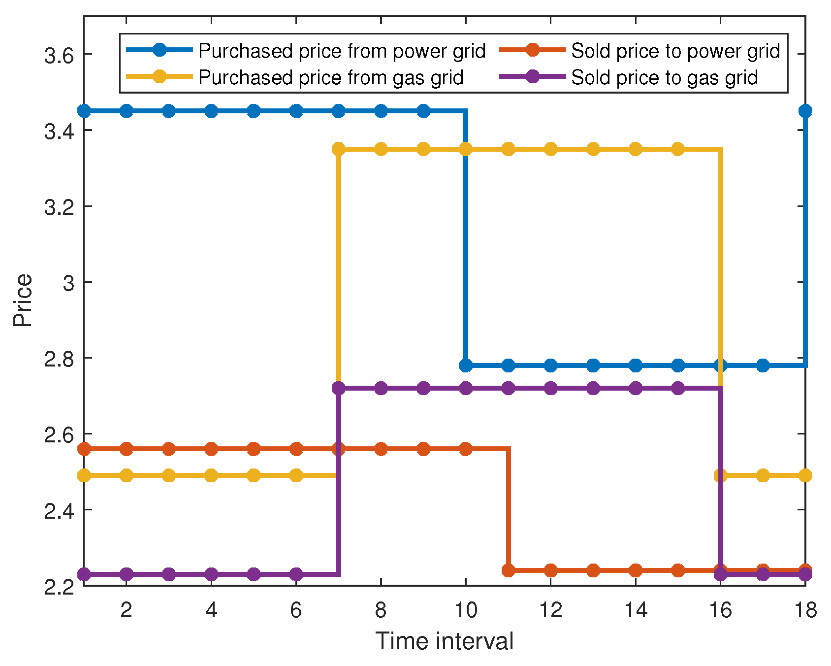
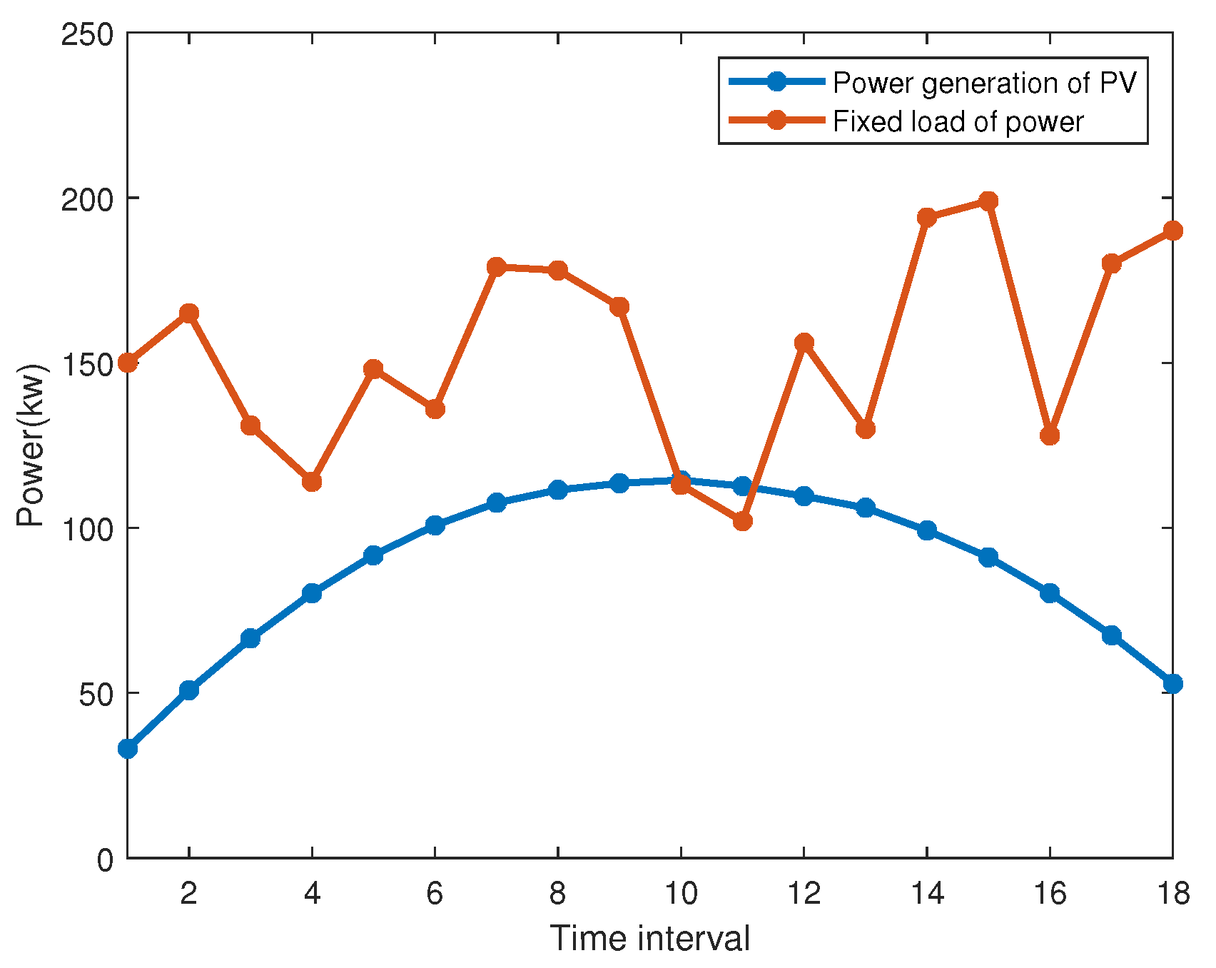
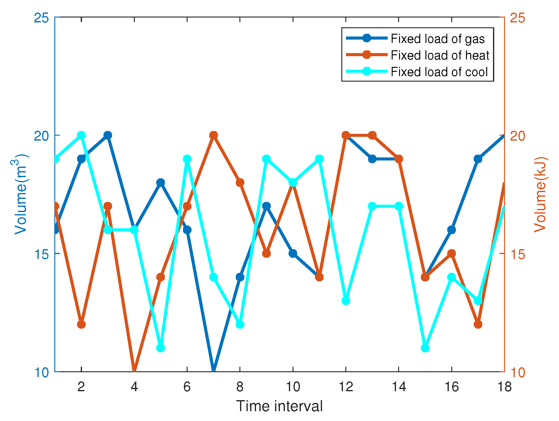
4.1. Simulation Setup

In this section, a lithium-ion battery production site with a lithium-ion battery assembly system, PV panels, BESS, CGT, P2G, EB, EC, GB, AC and WHB is considered. As shown in Figure 3, there are three assembly lines for assembling parts $(i=1,2,3)$ and a main product line for assembling parts obtained from the three assembly lines and further saturating, formating and grading in the lithium-ion battery assembly system. The production rate and power consumption rate of each machine are proposed in

Table 3. Parameters for tasks [25].

Task	Machine	Production Rate	Power Consumption Rate
Assembly I	$m_{11}$	35 Unit/h	22.8 kW/h
Assembly II	$m_{12}$	32 Unit/h	20.8 kW/h
Assembly III	$m_{13}$	40 Unit/h	25.6 kW/h
Assembly IV	$m_{21}$	30 Unit/h	26.2 kW/h
Assembly V	$m_{22}$	26 Unit/h	24.6 kW/h
Assembly VI	$m_{31}$	30 Unit/h	26.2 kW/h
Assembly VII	$m_{01}$	25 Unit/h	12.4 kW/h
Saturating	$m_{02}$	24 Unit/h	10.2 kW/h
Formation	$m_{03}$	30 Unit/h	13.6 kW/h
Grading	$m_{04}$	28 Unit/h	9.5 kW/h

, which come from [25]. For more information about the lithium battery system, please refer to [24,25] and their references. Assume the day-ahead scheduling horizon contains 9 h from 8:00 a.m. to 17:00 p.m., with $▵T=30$ min, which indicates that there are 18 time intervals, i.e., $T=18$. As in the model shown in Section 2.1, there are $c_{1,1}=[11.4,21.8,21.8,34.6,23.2,12.8,0_{1\times 12}]$, $c_{2,1}=[13.1,25.4,25.4,25.4,12.3,12.3,0_{1\times 12}]$, $c_{3,1}=[13.1,13.1,13.1,13.1,0_{1\times 14}]$ and $c_{0,1}=[6.2,11.3,11.3,18.1,22.85,$$16.65,11.55,4.75,4.75,0_{1\times 9}]$. In addition, the constraints between the component production lines and the assembly line are $\mathfrak{h}({\mathit{s}}_0-{\mathit{s}}_1)\ge 4$, $\mathfrak{h}({\mathit{s}}_0-{\mathit{s}}_2)\ge 2$, $\mathfrak{h}({\mathit{s}}_0-{\mathit{s}}_3)\ge 1$.

The parameters of the integer energy system come from [16], and the specific parameters are shown. The unit degradation cost of the BESS is $c_B=0.15$; the efficiency parameters of charging and discharging are ${\beta }_{B,c}={\beta }_{B,d}=0.9$; the maximum discharging and charging powers are $P_{dis,max}^{BESS}=35$ kW and $P_{cha,max}^{BESS}=40$ kW; the rated capacity is $E_{B,r}=50$ kWh; the maximum and minimum state of charging are $So{C}_{max}=1$, $So{C}_{min}=0.1$; the high heating value of natural gas is $HHV=33.5$ MJ/m³; the conversion coefficients of the CGT, WH, AC and WHB are ${\beta }_{CGT}=0.2428$, ${\beta }_{WH}=0.5$, ${\beta }_{AC}=1.3$ and ${\beta }_{WHB}=0.85$; and the conversion coefficient of P2G, the EB, EC and GB are ${\beta }_{P2G}=0.6$, ${\beta }_{EB}=0.9$, ${\beta }_{EC}=3$ and ${\beta }_{GB}=0.85$. The comprehensive heat transfer factor is $K=5$ W/m²; the building surface area and volume are $F=240$ m² and $V=360$ m³; the heat capacity of indoor air is $C_{air}=1.007$ kJ/(kg· K); and the density of indoor air is ${\rho }_{air}=1.2$ kg/m³. The outdoor temperature, the set indoor temperature and their differences are shown in Figure 4. The power and natural purchased prices and sold prices in different time periods are shown in Figure 5. Assume that photovoltaic power generation is certain, regardless of its volatility and uncertainty. The PV generation, the fixed electricity load, the fixed natural gas load, the fixed heating load and the fixed cooling load are shown in Figure 6 and Figure 7, in which the PV generation comes from the Desert Knowledge Australia Centre and the fixed loads are randomly generated within a certain range. In addition, the weight parameters are set as $W_1=W_2=0.5$.

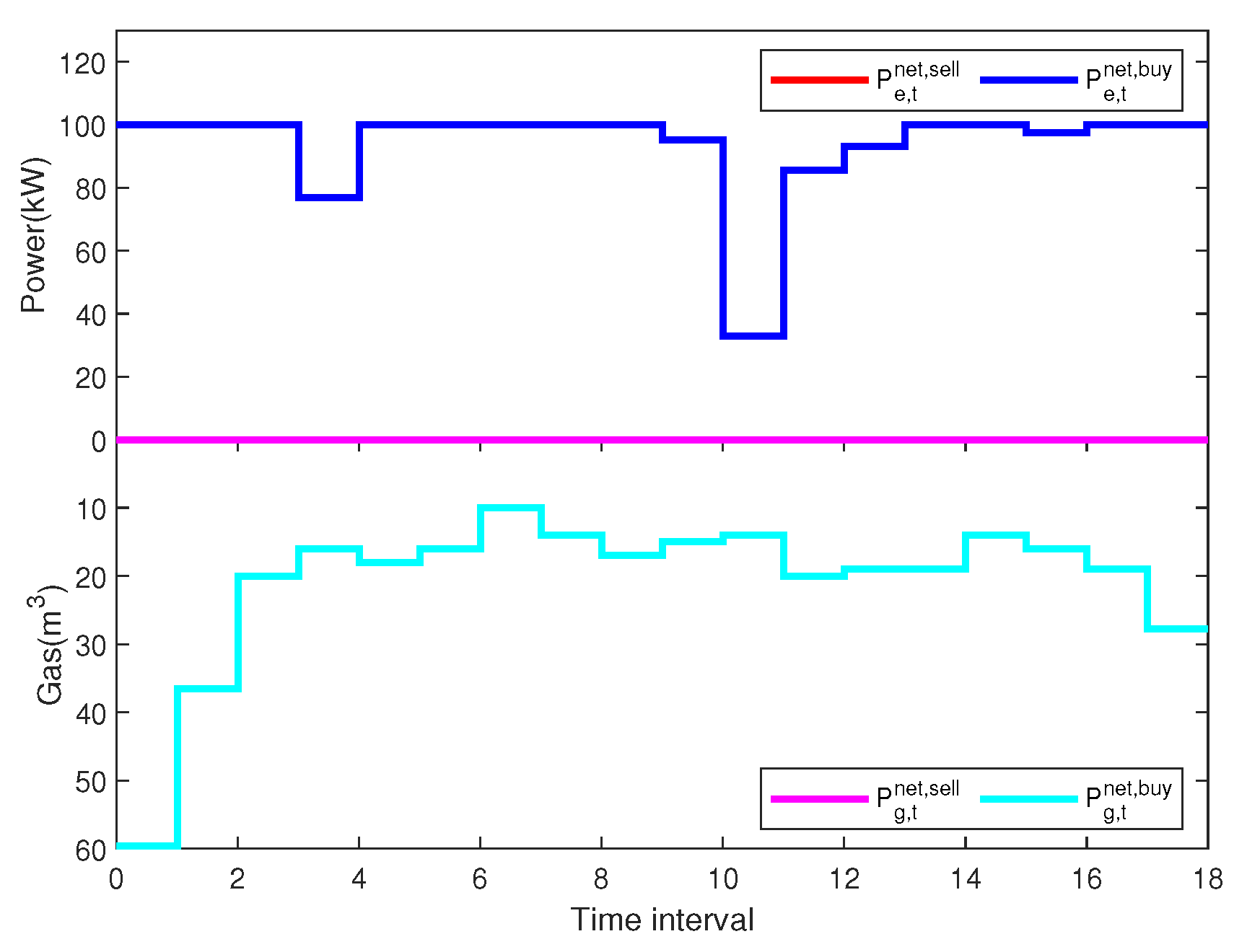
4.2. Simulation Result

The final scheduling results for the lithium-ion battery assembly production lines are $s_{1,3}=1$, $s_{2,7}=1$, $s_{3,8}=1$ and $s_{0,9}=1$. The other parameters are zero, i.e., the first production line turns on during the third time period, the second production line turns on during the seventh time period, the third production line turns on during the eighth time period and the final assembly line turns on during the ninth time period. Obviously, the time coupling constraints are fully satisfied, and the electricity load caused by TMAP can be calculated based on the given $c_{1,1}$, $c_{2,1}$, $c_{3,1}$ and $c_{0,1}$.

The charging and discharging power of the BESS during different time periods are shown in Figure 8. Obviously, the charging power and discharging power are not non-zero in the same time period, avoiding charging and discharging at the same time. Meanwhile, the states of charging in the dynamic scheduling process are always within the allowable range.

The results of the bought power from the utility electricity network, the sold power to the utility electricity network, the bought natural gas from the utility gas network and the sold natural gas to the utility gas network are shown in Figure 9. It should be noted that the sold power to the utility electricity network and the sold natural gas to the utility gas network are zero at all times. The reason for this phenomenon is that the area of photovoltaic panels is not large enough, or the light intensity is weak. There is not enough power to sell to the utility power network. On the other hand, the difference between indoor temperature and outdoor temperature is so large that a lot of heating or cooling load needs to be satisfied. Furthermore, the simulation results of $P_{g,t}^{CGT}$, $P_{g,t}^{GB}$ and $P_{e,t}^{EB}$ are shown in Figure 10, which is used to show the effectiveness of the proposed method.

In addition, two single-objective dispatch optimization problems have been chosen as the baseline strategies to show the necessity for considering comprehensive costs and carbon emissions. On the one hand, $E_{CDE}$ is regarded as the single minimum objective function, and the corresponding optimization problem with constraints (1)–(37) is solved to obtain the optimization value $E_{CDE}$. It is represented as single-objective model I. On the other hand, $C_{DCC}$ is also regarded as the single minimum objective function, and the corresponding optimization problem with constraints (1)–(37) is solved to obtain the optimization value $C_{DCC}$. It is represented as single-objective model II. The obtained results come from two single-objective dispatch optimization problems, and the proposed methods are shown in

Table 4. The values of $E_{CDE}$ and $C_{DCC}$ obtained in different models.

	Proposed Model	Single-Objective Model I	Single-Objective Model II
$E_{CDE}$	165.2898	155.9281	598.0418
$C_{DCC}$	6399.8	6602.1	6328.6

. According to Table 4, single-objective model I takes minimizing carbon emissions as the optimization goal, but its corresponding total operating costs are very high. Meanwhile, although single-objective model II has the lowest operating costs, its carbon emissions are too large. This is not conducive to environmental protection. Compared with them, the proposed model in this paper has a relatively low carbon emission value $E_{CDE}$, and the value of $C_{DCC}$ proposed in this paper is lower than that of single-objective model I and higher than that of single-objective model II. This fully demonstrates the need to consider carbon emissions and operating costs comprehensively.

5. Conclusions

In this paper, the dispatch of an integrated photovoltaic-gas-manufacturing facility system considering carbon emissions and operation costs is investigated. Two kinds of energy, electricity and natural gas, are contained in the integer energy system, in which the electricity mainly comes from the PV panels and the utility electricity network, and the natural gas mainly comes from the utility gas network. In addition, electricity and natural gas can be converted into each other. Four kinds of loads, electricity load, gas load, heating load and cooling load, need to be satisfied, in which the electricity load can be divided into the fixed load and flexible load. The flexible load comes from the scheduling for manufacturing facilities, and the scheduling of manufacturing facilities is modeled as a kind of deferable load to be integrated into the energy system. Moreover, daily operation costs and carbon emissions are considered in the decision, and the deviation preference strategy is used to solve this multi-objective optimization problem. Finally, a case study is proposed to show the effectiveness of the method. In the future, the issues will be further investigated. Firstly, the variability and uncertainty in the manufacturing task should be investigated. Secondly, the influence of building insulation, occupancy patterns and HVAC control dynamics should be considered. Thirdly, more types of manufacturing systems should be modeled.

References

1. Ufa, R.A.; Malkova, Y.Y.; Gusev, A.L.; Ruban, N.Y.; Vasilev, A.S. Algorithm for optimal pairing of res and hydrogen energy storage systems. Int. J. Hydrogen Energy 2021, 46, 33659–33669. [Google Scholar] [CrossRef]
2. Zhao, Z.Y.; Xia, L.C.; Jiang, L.Y.; Ge, Q.B.; Yu, F. Distributed bandit online optimisation for energy management in smart grids. Int. J. Syst. Sci. 2023, 54, 2957–2974. [Google Scholar] [CrossRef]
3. Liu, L.N.; Yang, G.H. Distributed energy resource coordination for a microgrid over unreliable communication network with dos attacks. Int. J. Syst. Sci. 2024, 55, 237–252. [Google Scholar] [CrossRef]
4. Lian, J.J.; Zhang, Y.S.; Ma, C.; Yang, Y.; Chaima, E. A review on recent sizing methodologies of hybrid renewable energy systems. Energy Convers. Manag. 2019, 199, 112027. [Google Scholar] [CrossRef]
5. Ahmad, A.; Khan, A.; Javaid, N.; Hussain, H.M.; Abdul, W.; Almogren, A.; Alamri, A.; Niaz, I.A. An optimized home energy management system with integrated renewable energy and storage resources. Energies 2017, 10, 549. [Google Scholar] [CrossRef]
6. Li, Y.; Wang, C.L.; Li, G.Q.; Wang, J.L.; Zhao, D.B.; Chen, C. Improving operational flexibility of integrated energy system with uncertain renewable generations considering thermal inertia of buildings. Energy Convers. Manag. 2020, 207, 112526. [Google Scholar] [CrossRef]
7. Gao, J.; Shao, Z.G.; Chen, F.X.; Lak, M. Energy trading strategies for integrated energy systems considering uncertainty. Energies 2025, 18, 935. [Google Scholar] [CrossRef]
8. Wang, M.; Yu, H.; Jing, R.; Liu, H.; Chen, P.D.; Li, C.E. Combined multi-objective optimization and robustness analysis framework for building integrated energy system under uncertainty. Energy Convers. Manag. 2020, 208, 112589. [Google Scholar] [CrossRef]
9. Yang, J.; Zhang, G.S.; Ma, K. Hierarchical dispatch using two-stage optimisation for electricity markets in smart grid. Int. J. Syst. Sci. 2016, 47, 3529–3536. [Google Scholar] [CrossRef]
10. Liang, P.R.; Zhang, H.H.; Liang, R. Cooperative game enabled low-carbon energy dispatching of multi-regional integrated energy systems considering carbon market. Energies 2025, 18, 759. [Google Scholar] [CrossRef]
11. Jiang, P.; Dong, J.; Huang, H. Optimal integrated demand response scheduling in regional integrated energy system with concentrating solar power. Appl. Therm. Eng. 2020, 166, 114754. [Google Scholar] [CrossRef]
12. Zhang, N.; Sun, Q.Y.; Yang, L.X. A two-stage multi-objective optimal scheduling in the integrated energy system with We-Energy modeling. Energy 2021, 215, 119121. [Google Scholar] [CrossRef]
13. Li, Y.; Han, M.; Yang, Z.; Li, G.Q. Coordinating flexible demand response and renewable uncertainties for scheduling of community integrated energy systems with an electric vehicle charging station: A bi-level approach. IEEE Trans. Sustain. Energy 2021, 12, 2321–2331. [Google Scholar] [CrossRef]
14. Huang, H.X.; Liang, R.; Lv, C.X.; Lu, M.T.; Gong, D.W.; Yin, S.L. Two-stage robust stochastic scheduling for energy recovery in coal mine integrated energy system. Appl. Energy 2021, 290, 116759. [Google Scholar] [CrossRef]
15. Li, B.; Li, X.; Su, Q.Y. A system and game strategy for the isolated island electric-gas deeply coupled energy network. Appl. Energy 2022, 306, 118013. [Google Scholar] [CrossRef]
16. Zhu, G.; Gao, Y.; Sun, H. Optimization scheduling of a wind-photovoltaic-gas-electric vehicles community-integrated energy system considering uncertainty and carbon emissions reduction. Sustain. Energy Grids Netw. 2023, 33, 100973. [Google Scholar] [CrossRef]
17. Naderi, E.; Azizivahed, A.; Asrari, A. A step toward cleaner energy production: A water saving-based optimization approach for economic dispatch in modern power systems. Electr. Power Syst. Res. 2022, 204, 107689. [Google Scholar] [CrossRef]
18. Naderi, E.; Mirzaei, L.; Trimble, J.P.; Cantrell, D.A. Multi-objective optimal power flow incorporating flexible alternating current transmission systems: Application of a wavelet-oriented evolutionary algorithm. Electr. Power Compon. Syst. 2024, 52, 766–795. [Google Scholar] [CrossRef]
19. Duan, P.F.; Feng, M.D.; Zhao, B.X.; Xue, Q.W.; Li, K.; Chen, J.L. Operational optimization of regional integrated energy systems with heat pumps and hydrogen renewable energy under integrated demand response. Sustainability 2024, 16, 1217. [Google Scholar] [CrossRef]
20. Yang, J.; Li, C.H.; Ma, K.; Liu, H.R.; Guo, S.L. Multi-energy pricing strategy for port integrated energy systems based on contract mechanism. Energy 2024, 290, 130114. [Google Scholar] [CrossRef]
21. Liu, L.Z.; Su, X.L.; Chen, L.J.; Wang, S.; Li, J.W.; Liu, S.W. Elite genetic algorithm based self-sufficient energy management system for integrated energy station. IEEE Trans. Ind. Appl. 2024, 60, 1023–1033. [Google Scholar] [CrossRef]
22. Sun, Q.R.; Wu, Z.; Gu, W.; Zhang, X.P.; Lu, Y.A.; Liu, P.; Lu, S.; Qiu, H.F. Resilience assessment for integrated energy system considering gas-thermal inertia and system interdependency. IEEE Trans. Smart Grid 2024, 15, 1509–1524. [Google Scholar] [CrossRef]
23. Shafie-Khah, M.; Siano, P.; Aghaei, J.; Masoum, M.A.S.; Li, F.X.; Catalao, J.P.S. Comprehensive review of the recent advances in industrial and commercial DR. IEEE Trans. Ind. Inform. 2019, 15, 3757–3771. [Google Scholar] [CrossRef]
24. Li, Y.C.; Hong, S.H. Real-time demand bidding for energy management in discrete manufacturing facilities. IEEE Trans. Ind. Electron. 2017, 64, 739–749. [Google Scholar] [CrossRef]
25. Lu, R.Z.; Li, Y.C.; Li, Y.T.; Jiang, J.H.; Ding, Y.M. Multi-agent deep reinforcement learning based demand response for discrete manufacturing systems energy management. Appl. Energy 2020, 276, 115473. [Google Scholar] [CrossRef]
26. Ding, Y.M.; Hong, S.H.; Li, X.H. A demand response energy management scheme for industrial facilities in smart grid. IEEE Trans. Ind. Inform. 2014, 10, 2257–2269. [Google Scholar] [CrossRef]
27. Yu, M.M.; Lu, R.Z.; Hong, S.H. A real-time decision model for industrial load management in a smart grid. Appl. Energy 2016, 183, 1488–1497. [Google Scholar] [CrossRef]
28. Huang, C.; Zhang, H.C.; Song, Y.H.; Wang, L.; Ahmad, T.; Luo, X. Demand response for industrial micro-grid considering photovoltaic power uncertainty and battery operational cost. IEEE Trans. Smart Grid 2021, 12, 3043–3055. [Google Scholar] [CrossRef]
29. Wu, Q.; Song, Q.K. Isolated industrial micro-grid demand response with assembly process based on distributionally robust chance constraint. Int. J. Syst. Sci. 2024, 55, 2211–2223. [Google Scholar] [CrossRef]
30. Wu, Q.; Song, Q.K.; He, X.; Chen, G.; Huang, T.W. Distributed peer-to-peer energy trading framework with manufacturing assembly process and uncertain renewable energy plants in multi-industrial micro-grids. Energy 2024, 302, 131876. [Google Scholar] [CrossRef]
Figure 1. Schematic diagram of the integrated energy system.
Energies 18 02224 g001
Figure 2. Assembly process in practical manufacturing environments [28].
Energies 18 02224 g002
Figure 3. Lithium-ion battery assembly system.
Energies 18 02224 g003
Figure 4. The set suitable indoor temperature, predicted outdoor temperature and the temperature difference.
Energies 18 02224 g004
Figure 5. The purchased prices from grid and sold prices to the grid.
Energies 18 02224 g005
Figure 6. The power generated by PV and the fixed load of power.
Energies 18 02224 g006
Figure 7. The fixed load of natural gas, heating and cooling.
Energies 18 02224 g007
Figure 8. The charging and discharging power of the BESS.
Energies 18 02224 g008
Figure 9. The purchased power and gas from the utility network, and the sold power and gas to the utility network.
Energies 18 02224 g009
Figure 10. The simulation results of P g , t C G T , P g , t G B and P e , t E B .
Energies 18 02224 g010