1. Introduction
Four wire delta services are still used in North America for electric power distribution in manufacturing industries and residential and commercial facilities. This service generally is built by three single-phase transformers [
1], whose primary and secondary windings are connected in delta, but one of these transformers has three secondary terminals (
), since the secondary winding has a mid-tap terminal where a neutral conductor can be connected. The fourth secondary terminal of the transformer (
) is known as the wild leg or high leg terminal. The primary windings of the transformer could be connected in wye [
1], but this configuration is less used in practice than delta; thus, in this paper, only the primary delta connection has been considered. The four-wire delta (4WD) transformer supplies single-phase loads, such as residential, commercial and lighting loads, which are connected to
and
phases and the neutral wire,
(unbalanced wye load). The high leg terminal
) is not generally used because of its voltage is
times higher than
and
. The line to neutral voltages,
and
, are opposite ones and their nominal RMS values are half of the nominal RMS line to line voltages (
). The line to line voltages are almost balanced and they are usually applied to supply three-phase loads, as electrical motors. The most usual RMS voltages for 4WD services are 120 V (
phases to neutral) and 240 Vac (line to line voltages) [
2]; then, the high leg RMS voltage is 208 V. Other nominal RMS voltages used in USA for 4WD services [
2] are 240 V/480 V/415 V (high leg).
The 4WD service operation and optimization off-line simulator described in this paper runs in Excel, but another version in LABVIEW is available. The Excel version of the simulator is suitable to for use by engineers and technicians in simulating and verifying the operation of 4WD services. LABVIEW version is applied to implement measuring instruments, as power analyzers. Both simulator versions, Excel and LABVIEW, manage the same formulations. Kirchhoff’s Laws are used to calculate voltages, currents and voltage drops in the secondary windings of the 4WD transformer, as well as in the loads and lines. The magnetic equations of the transformer are applied to determine the primary winding currents. The nominal specifications of the transformer, loads and lines are previously inserted in particular boxes in both simulator versions, which are data to solve Kirchhoff’s equations.
Transformer cooper losses and LV line losses are obtained according to the winding currents, obtained from Kirchhoff’s Laws. The transformer primary and secondary power losses can have different values due to the secondary neutral current, and the same occurs with the apparent powers measured either from the primary or the secondary, because of the different primary and secondary imbalances caused by the neutral current. The primary apparent powers have been obtained using the voltages and currents calculated in the primary windings, according to Buchholz’s [
3] or unified power measurement (UPM) formulation [
4]. Those powers would have the same values applying either Emanuel’s [
5,
6] or IEEE Standard 1459 [
7] or Czarnecki and Haley’s [
8] formulations to the HV line voltages and currents. The secondary apparent power has been obtained using an original power formulation derived from Buchholz’s that uses the LV line and neutral currents instead of the secondary winding currents, which is advantageous, in our opinion, since it is generally difficult to measure the secondary winding currents in practice. The total apparent power of both loads, wye and delta, is determined as the vector sum of the UPM apparent power vectors of each load [
9,
10]; the utilization of the apparent powers in vector notation is a technical innovation included in this paper and is necessary since this service applies very different voltage imbalances to each load.
The optimization of the 4WD service operation is achieved in this simulator in two complementary ways: (1) distributing the wye loads between
and
phases, and (2) connecting passive reactive and unbalanced compensators. The first procedure allows to cancel (or, at least, to minimize) the neutral current originated by the wye loads. The reactive and unbalanced compensators must minimize the positive-sequence reactive currents and the negative-sequence currents supplied to the wye and delta loads. Those passive compensators are built by three-phase delta connections of coils and capacitors, whose values are determined in the same manner as it was explained in references [
11,
12,
13]. Our compensators are connected in delta for two reasons, mainly: (1) to simplify the topology; and (2) to apply quasi-balanced line to line voltages to the elements of those devices.
The simulator is able to determine the elements of the optimal equivalent wye load as well as the necessary passive compensators to optimize the operation of the 4WD service. The resulting elements of both optimization techniques and compensation devices are presented in the simulator in separate boxes and they can be incorporated to the system in order to evaluate their effects. Three passive compensators for each load (wye and delta) may be independently selected by the simulator users: reactive compensator only, unbalanced compensator only and combined reactive and unbalanced compensator; thus, a wide range of possibilities are at the disposal of the user for analyzing the 4WD service in sinusoidal steady-state operation.
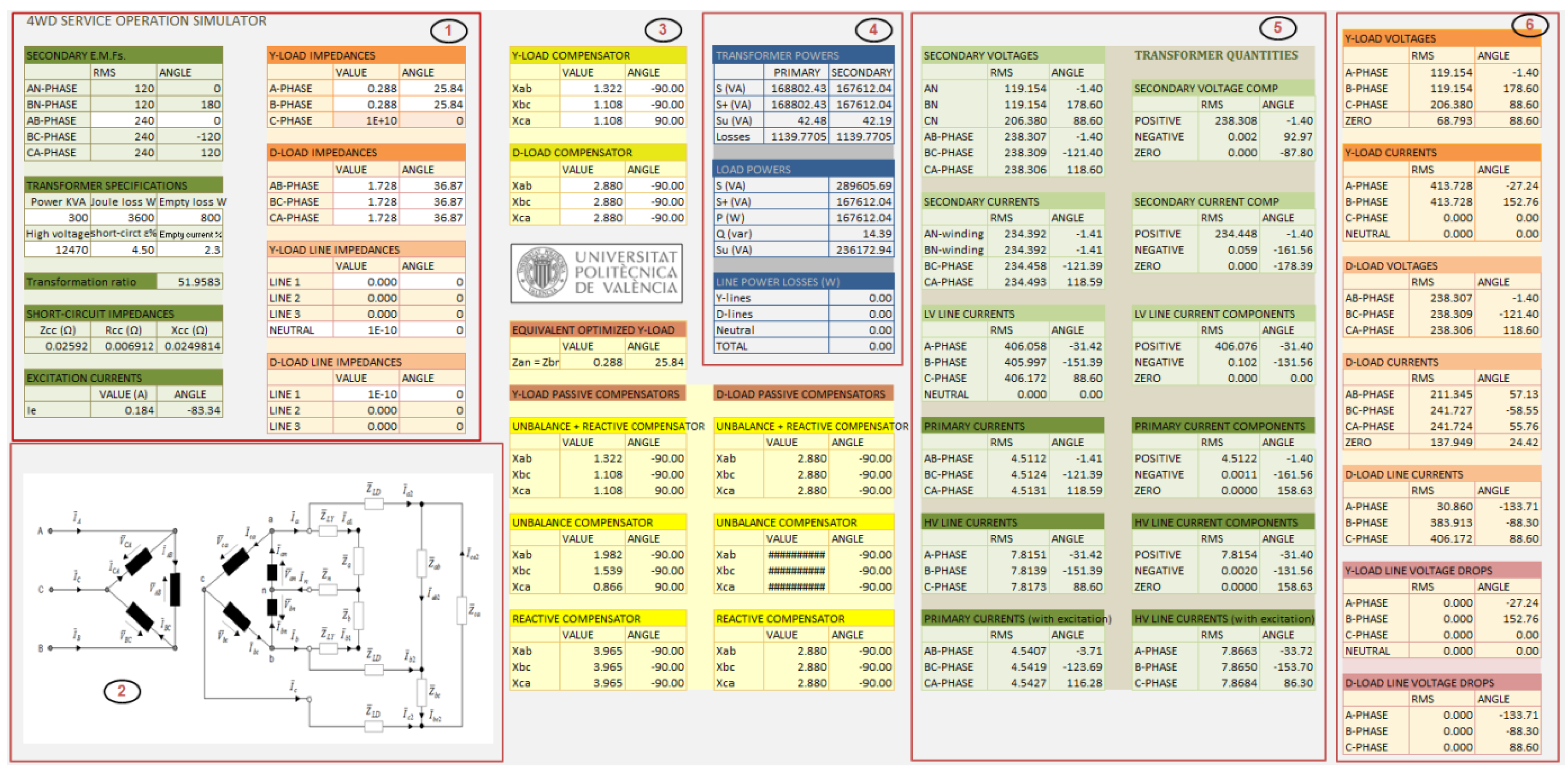
The specifications (rated powers, voltages, impedances,
etc.) of the transformer, lines and loads as well as the responses (voltages, currents, powers and losses) in those parts of the 4WD service are presented in different distinctive colored boxes in the simulator (
Figure 1), in order to easily manage the simulator.
2. Structure of Simulator
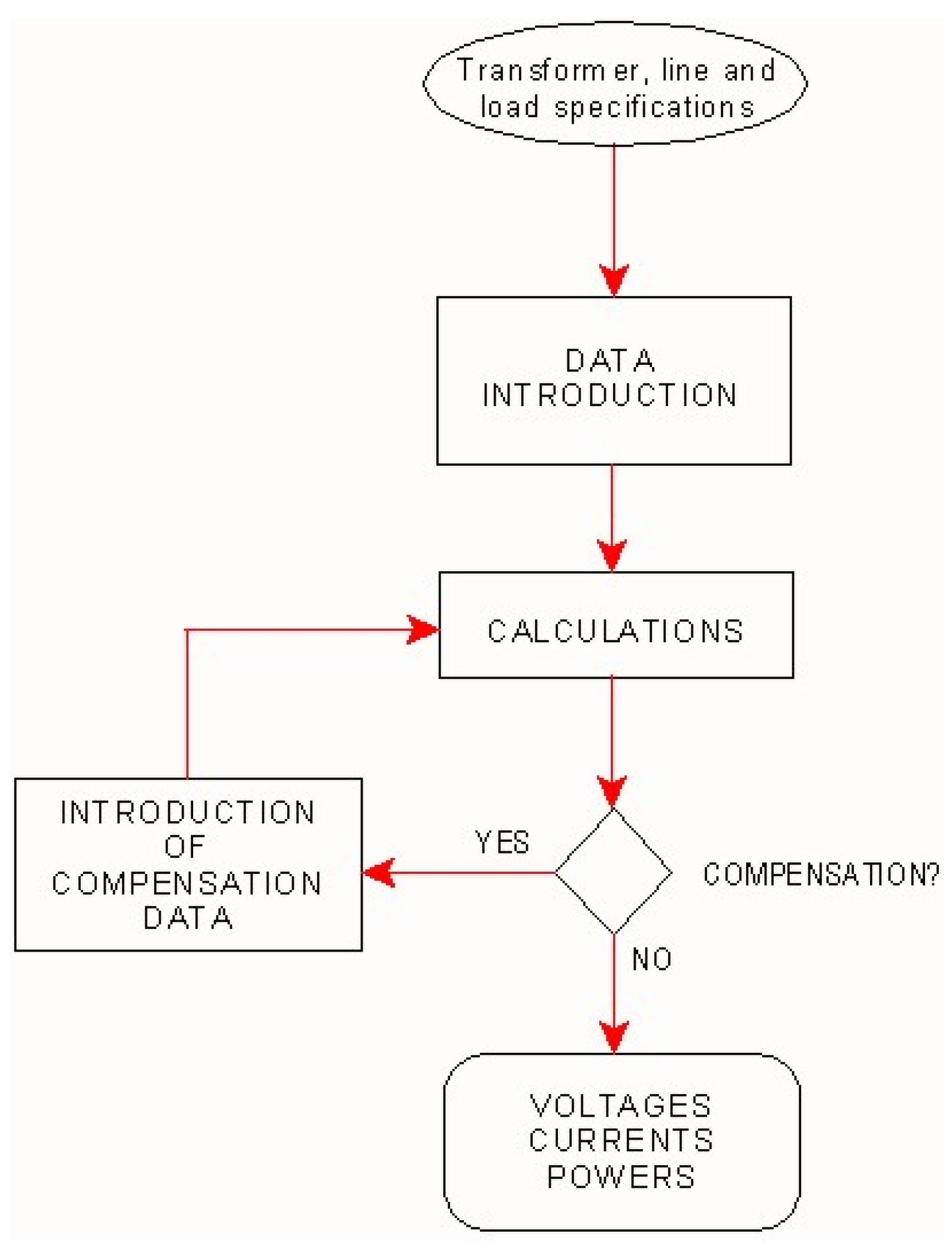
The block diagram of the simulator is represented in
Figure 2. The introduction of the transformer, line and load specifications is the first step in the simulation process. Those data are included on the circuit loop equations, in the “Calculation” block, in which the voltages, currents and powers in all parts of the 4WD service are calculated. Also, the elements of the reactive and unbalanced passive compensators as well as the optimal distribution of the wye load are determined in the “Calculation” block according to the load specifications. If the compensation is not required, the voltages, currents and powers in each part of the 4WD service are displayed in specific boxes. Whether the compensation effects have to be analyzed, the elements of a selected compensator (reactive, unbalanced or integral) for each load can be included in the loop equations and, thus, the new values of the voltages, currents and powers in the 4WD service are calculated and displayed.
Figure 1.
Four-wire delta (4WD) service simulator main page: (1) transformer, line and load specifications; (2) scheme; (3) compensation area; (4) transformer, line and load powers; (5) transformer voltages and currents; (6) line and load voltages and currents. “####” is infinite value.
Figure 1.
Four-wire delta (4WD) service simulator main page: (1) transformer, line and load specifications; (2) scheme; (3) compensation area; (4) transformer, line and load powers; (5) transformer voltages and currents; (6) line and load voltages and currents. “####” is infinite value.
Figure 2.
Block diagram of the 4WD service simulator.
Figure 2.
Block diagram of the 4WD service simulator.
3. Transformer, Load and Line Specifications
Transformer, lines and load specifications provided by the manufacturers can be manually inserted in specific boxes of the simulator (
Figure 1). Those quantities are necessary to solve the loop equations of the 4WD service circuit, as it will be described in
Section 4.
The main transformer quantities that should be included in the simulator in order to solve the circuit equations are the following:
- -
The transformer rated power (),
- -
The primary () and empty secondary () line to line RMS voltages,
- -
The short-circuit voltage (, in percent of the nominal voltages), and
- -
The nominal cooper losses ().
The transformer secondary e.m.fs. are defined in the simulator introducing only the empty secondary line to line RMS voltages in the transformer specification box (
Figure 1), since:
being
. According to the primary and empty secondary line to line RMS voltages the transformation ratio (
) is determined:
The transformer combined impedance seen from the secondary (
) and its components (
) are respectively obtained as:
The empty power losses (
) and the excitation (empty) current (
) as percentages of the nominal primary current are additional quantities that can be inserted in the transformer specification boxes. Those quantities allow calculating the RMS value and angle of the primary excitation currents:
The load impedances can be introduced in the load specification boxes of the calculator (
Figure 1) in two ways: (1) directly, inserting their values and angles, and (2) according to the nominal voltages (
), active powers (
) and power factors (
) of those impedances; such as the complex impedance of a load placed in the
z-phase is:
The load impedance corresponding to the c-phase in the wye connection is always considered infinite (i.e., empty circuit).
The complex impedances of the LV lines (
) and neutral (
) conductor are manually inserted in their specific boxes (
Figure 1). The lines corresponding to the wye (
Y) and delta (
D) circuits are independent ones; thus, their impedances (
) could have different values. The three phases of each line have the same impedances; however, the neutral impedance of the wye circuit could be different to the line impedances.
Although most loads create distorted currents in power systems, such as those supplied through electronic drives, their equivalent impedances, calculated from the fundamental-frequency voltages and currents, could be used for those loads too, in our opinion, since the non-fundamental phenomena are not analyzed in this paper. We agree with the IEEE Standard 1459 [
7] that the active, reactive and unbalanced power phenomena should be defined and measured for the fundamental-frequency.
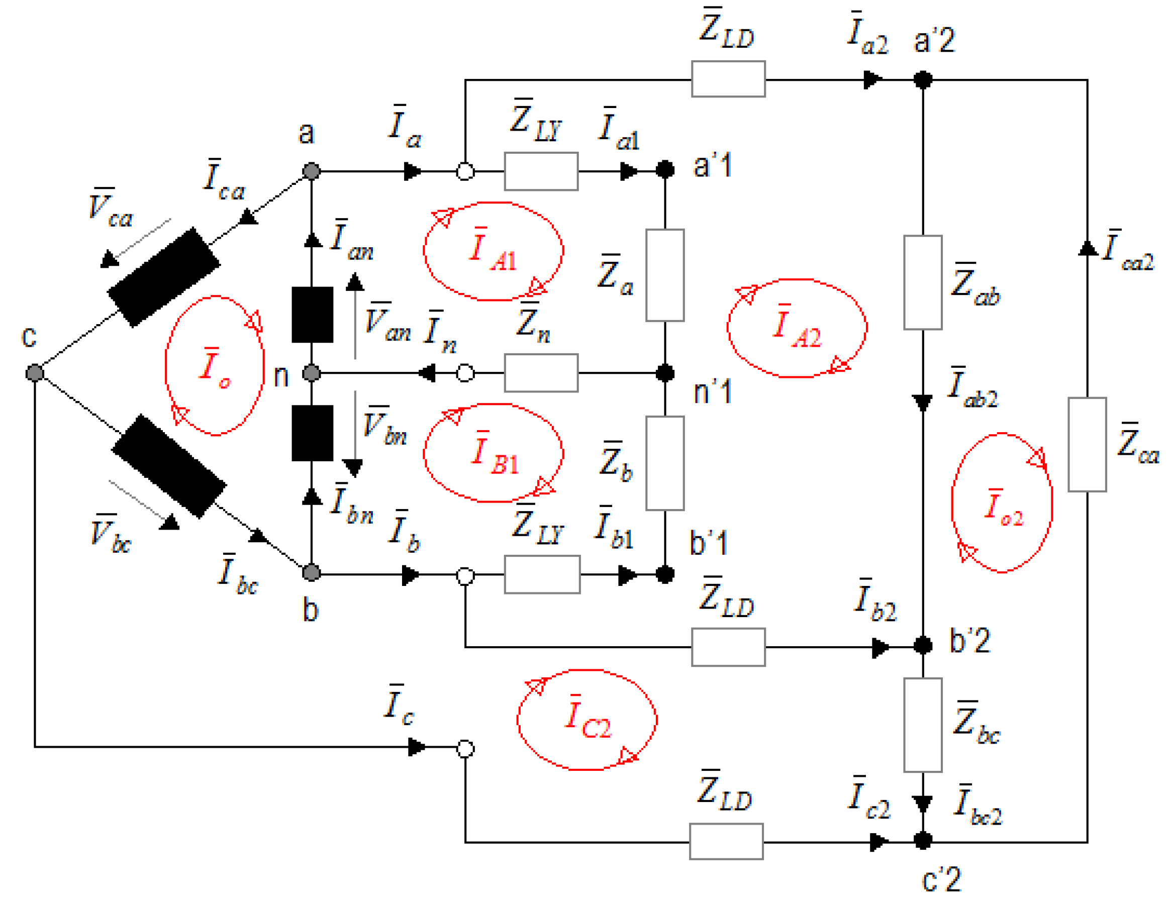
4. Four-Wire Delta (4WD) Service Analysis Equations
The currents in the transformer windings, in the lines and loads are the basic quantities that allow determine the voltages, powers and power loses in the 4WD service. Those currents can be calculated from the following six equations corresponding to the loops of the circuit formed by the secondary side of the transformer, the LV lines and loads (
Figure 3), which are derived from the second Kirchhoff’s Laws:
There is no loop equation corresponding to the third phase of the wye load that would be connected to the high leg terminal (), by simplicity, because of any impedance of the wye load is generally supplied by that terminal. The unknown quantities in the above equations are the Complex RMS CRMS values of the loop currents: .
The CRMS values of the secondary e.m.fs. of the transformer,
, as well as the complex combined impedance of the transformer,
, the complex wye load impedances (
), the complex delta load impedances (
) and the complex line and neutral impedances (
) expressed in Equation (6) are known quantities, obtained from the transformer load and line specifications, respectively, such as it was indicated in
Section 3.
Figure 3.
4WD service: secondary circuit scheme and loop currents.
Figure 3.
4WD service: secondary circuit scheme and loop currents.
5. Determination of Four-Wire Delta (4WD) Service Voltages, Currents and Powers
In this section, the equations used by the simulator for obtaining voltages, currents and powers in each part of the 4WD service are described. The resulting quantities are displayed in Equations (4)–(6) areas of the simulator main page (
Figure 1).
5.1. High Voltage (HV) Line and Transformer Voltages, Currents and Powers
The transformer secondary currents are calculated from the loop currents of Equation (6), according to:
According to the transformer magnetic equations, the primary currents are expressed as:
where
and
are the spires of primary and secondary, respectively, and
is the transformation ratio. Also, the HV line currents are, according to the First Kirchhoff’s Law:
The transformer secondary voltages are obtained as:
The primary line to line voltages () are considered balanced, of positive-sequence, and with approximately the same RMS value than the primary e.m.fs., , included in the transformer specifications. This approximation can usually be accepted in practice, because of the small primary voltage drops.
The 4WD transformer primary and secondary apparent powers are not generally the same, because of the neutral current, which creates different primary and secondary imbalances. The 4WD transformer apparent power calculated from the primary quantities is expressed as:
The 4WD transformer apparent power calculated from the secondary is obtained in the simulator in function of the LV line and neutral currents (
instead of the secondary winding currents
:
being:
and
,
are the positive and negative-sequence components of the LV line currents
).
The set of currents in Equation (12) causes the same transformer cooper power losses (
) as the secondary winding currents,
i.e.:
The above equality is verified because of the following relationships between the secondary winding currents and the LV line and neutral currents:
The cooper power losses calculated according to the primary winding currents are:
where
is the transformer combined resistance seen from the primary. Equations (13) and (15) provide the same values of transformer cooper power losses when the LV neutral current
) is zero.
The positive, negative and zero-sequence components of the primary winding currents (
) are obtained from Fortescue’s theorem [
14]. There are no zero-sequence components in the primary winding currents (
), and the same occurs with the set of secondary currents (
), whose symmetrical components (
) are the primary symmetrical components multiplied by the transformation ratio (
), according to Equation (8); thus,
.
The primary and secondary positive-sequence apparent powers (
) are respectively calculated from:
Differences observed between the values of the above powers are due to the different primary and secondary positive-sequence voltages (), caused by the transformer voltage drops.
The primary and secondary unbalanced powers (
) are obtained as:
5.2. Low Voltage (LV) Line and Load Voltages, Currents and Powers
The LV line and neutral currents are, according to the loop currents in Equation (6):
Notice there is no line current corresponding to the c-phase of the wye load, because of any impedance is connected to that wye load phase (
Figure 1).
The LV line voltage drops are calculated according to Ohm’s Law:
Delta load circuit:
being
and
the complex LV line impedances corresponding to the wye and delta load circuits, respectively, and
is the complex neutral impedance.
The LV line and neutral power losses are:
Neutral wire:
where
,
and
are the real part of the LV line
,
) and neutral (
) complex impedances, respectively.
The currents in the wye load phases (
) are those calculated from Equation (19) and the currents in the delta load phases are expressed as a function of the loop currents in Equation (6) as:
The voltages applied to the loads are determined by the simulator as:
Because of there are two topologies for the three-phase loads (wye and delta) in the 4WD service, an apparent power could be separately expressed for each of them and their values could be calculated using Buchholz or UPM formulations [
3,
4]; however, the total impact of those loads cannot be obtained as the arithmetic sum of the apparent powers of each load. On the other hand, since each load (wye and delta) is subjected to different voltages (very unbalanced for the wye loads and quasi-balanced for the delta loads), a combined apparent power formulation using either the line to neutral voltages or the line to line voltages or a combined set of both voltages would lead to wrong apparent power values. Last one could be the case, in our opinion, of the apparent power formulations presented in references [
5,
6,
7], because of the effective voltages run with estimated load parameters (
). Also, reference [
8] could not be used. The above problem can be avoided, in our opinion, using a vector apparent power formulation; because of the total load impact in the 4WD service could be determined as the vector sum of the vector apparent powers of each load. Fortunately, an unbalanced power vector (
) was formulated in references [
9,
10] and, thus, the apparent power (
) could be expressed in vector notation as:
where:
is the UPM unbalanced power vector [
10].
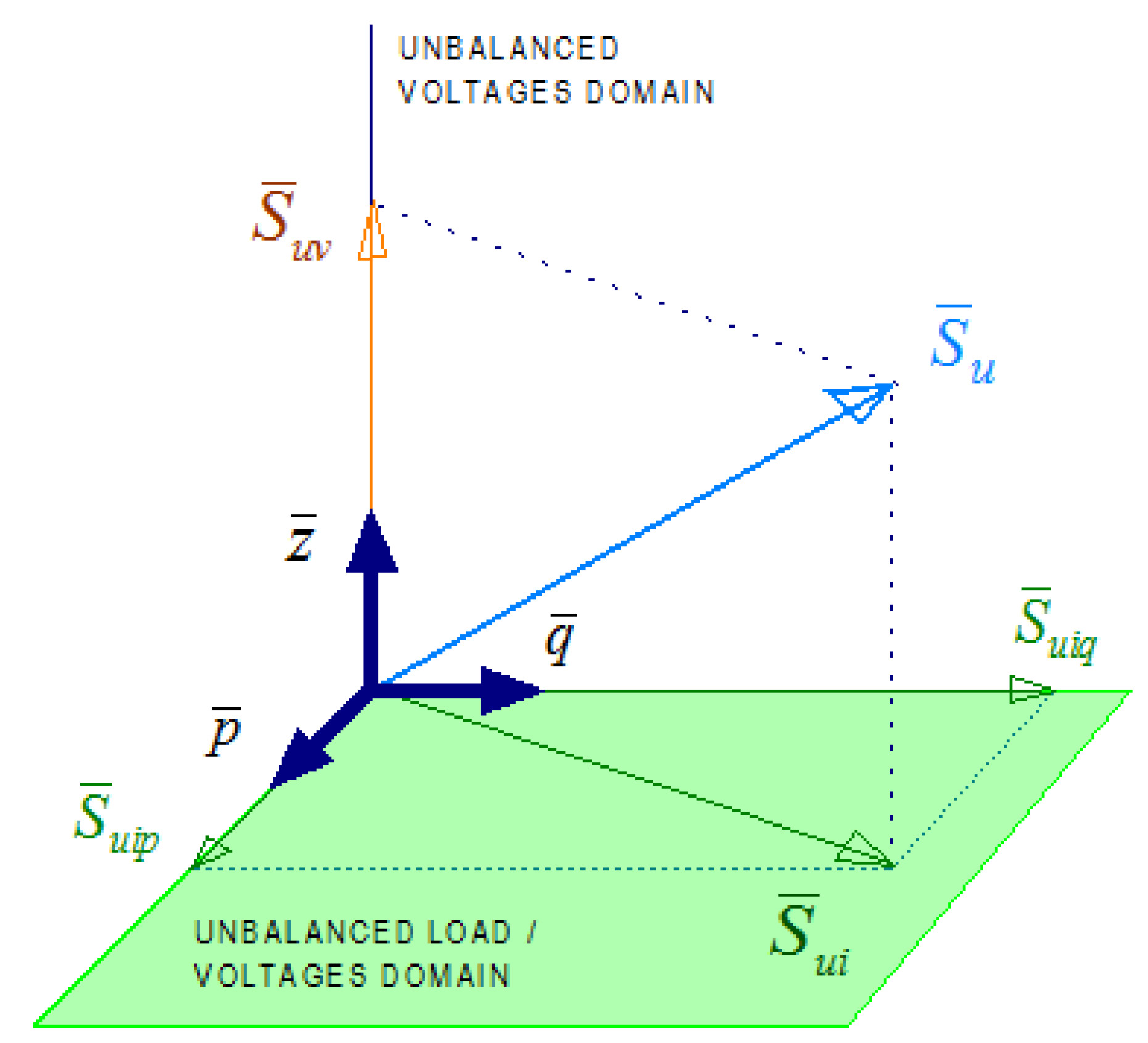
The unbalanced power components
and
represented in the plane described by the
axes in the above expression (
Figure 4) express the amount of the unbalance power due to the combined effects of voltage and load imbalances; while the term defined on the
axe measures the exclusive effects of the voltage imbalances (
).
are the positive-sequence active and reactive powers corresponding to each phase (
),
i.e.:
being
the CRMS positive-sequence voltage and
the conjugate of the CRMS positive-sequence current corresponding to the z-phase,
i.e.:
and
. The parameters
and
are the voltage unbalance and asymmetrical degrees, respectively:
which are respectively obtained as the relationship between the RMS negative- (
) and the zero-sequence (
) voltages and the RMS positive-sequence voltage (
). Between double bars in Equation (30) is expressed the norm of a vector o complex quantity.
is the positive-sequence complex apparent power:
The norm of the UPM apparent power vector (
) defined by Equation (29) holds the same value as Buchholz’s apparent power [
3].
The apparent power of the combined wye (
) and delta (
) loads is obtained in the simulator, according to Equation (29), as the vector sum of the apparent power vectors corresponding to the wye (
) and delta (
) loads:
The norm of that vector (
) is the apparent power of the combined load:
The norm of the unbalanced power vector (
) is the unbalanced power of the combined load:
and the positive-sequence apparent power of the combined load (
):
Figure 4.
Representation of the unified power measurement (UPM) unbalanced power vector and its components.
Figure 4.
Representation of the unified power measurement (UPM) unbalanced power vector and its components.
6. Reactive and Imbalance Load Compensation Devices and Methods
In this section, the simplest reactive and unbalance power compensation devices and methods are described and their elements formulated in order to minimize the currents in the transformer and mains and, then, to optimize the 4WD service operation.
The simplest reactive and imbalance compensators for each load (wye and delta) are formed by three-phase connections of coils and capacitors. The elements of those devices are connected in delta to the secondary of the transformer; thus, they are subjected to quasi-balanced line to line voltages and they supply either the reactive positive-sequence or the negative-sequence or both currents absorbed by those loads.
The line currents of the delta loads do not have zero-sequence components, but the currents supplied to the wye loads have zero-sequence components when the loads connected to the
and
-phases are different ones. Those zero-sequence currents could be compensated by passive elements such as are described in reference [
11], but the simplest compensation method is to equitably distribute the wye loads. The simulator presented in this paper provides the impedance values of the optimal wye load that minimizes the zero-sequence line currents.
The elements of the compensation devices and methods described in this section are displayed in specific boxes in the simulator and they can be selected and manually introduced in order to evaluate the compensation effects on the transformer and mains. The inclusion of those reactive and unbalance passive compensators in real-time environments would cause similar impacts as those created by the capacitor banks used for reactive power compensation.
6.1. Wye Load Compensation
The negative-sequence line currents supplied to the impedances
and
of the wye load are the same as those absorbed by a single-phase load (
):
which is connected between
and
transformer secondary terminals.
Assuming
and
) are the equivalent parallel resistance and reactance of
, the elements (
,
) of the wye load reactive and unbalance (negative current) compensators have the formulations expressed in
Table 1, according to references [
12,
13].
The zero-sequence line currents are supplied to the wye loads only and they are caused by the different values of wye load impedances. To minimize those currents, it is necessary to distribute the wye impedances up to an optimal value:
Table 1.
Reactive, unbalance (negative-sequence) and integral (reactive + unbalance) compensators for the wye loads.
Table 1.
Reactive, unbalance (negative-sequence) and integral (reactive + unbalance) compensators for the wye loads.
| Elements | Reactive compensator | Unbalance compensator | Integral compensator |
|---|
| | | |
| | | |
| | | |
The connection of the above impedances cancel (or minimize, at least) the zero-sequence line currents absorbed by the wye load, but they do not modify the value of the reactive and negative-sequence currents, whose compensation must be fulfilled by the devices shown in
Table 1.
6.2. Delta Load Compensation
The line currents absorbed by the delta loads only have positive (active and reactive) and negative components, but there are no zero-sequence components in those currents. The reactive and negative line currents can be minimized by three-phase delta compensators, connected to the secondary terminals and whose element formulations are expressed in
Table 2 in function of the conductance (
) and the susceptance (
) of each load phase [
12,
13],
i.e.:
Table 2.
Reactive, unbalance (negative-sequence) and integral (reactive + unbalance) compensators for the delta loads.
Table 2.
Reactive, unbalance (negative-sequence) and integral (reactive + unbalance) compensators for the delta loads.
| Elements | Reactive compensator | Unbalance compensator | Integral compensator |
|---|
| | | |
| | | |
| | | |
The formulations of passive reactive and unbalance compensators expressed in
Table 1 and
Table 2 for non-variable loads could be extended to variable loads such as it is indicated in reference [
15].
7. Application Example
The operation of a 300kVA 4WD service is analyzed in this section as an application of the simulator utilization, when it supplies two 120 V, 60 kVA (
PF = 0.9) and 40 kVA (
PF = 0.9) single-phase loads (lighting and residential installations), respectively connected between
and
phases and the neutral
), and a 240 V, 100 kVA (
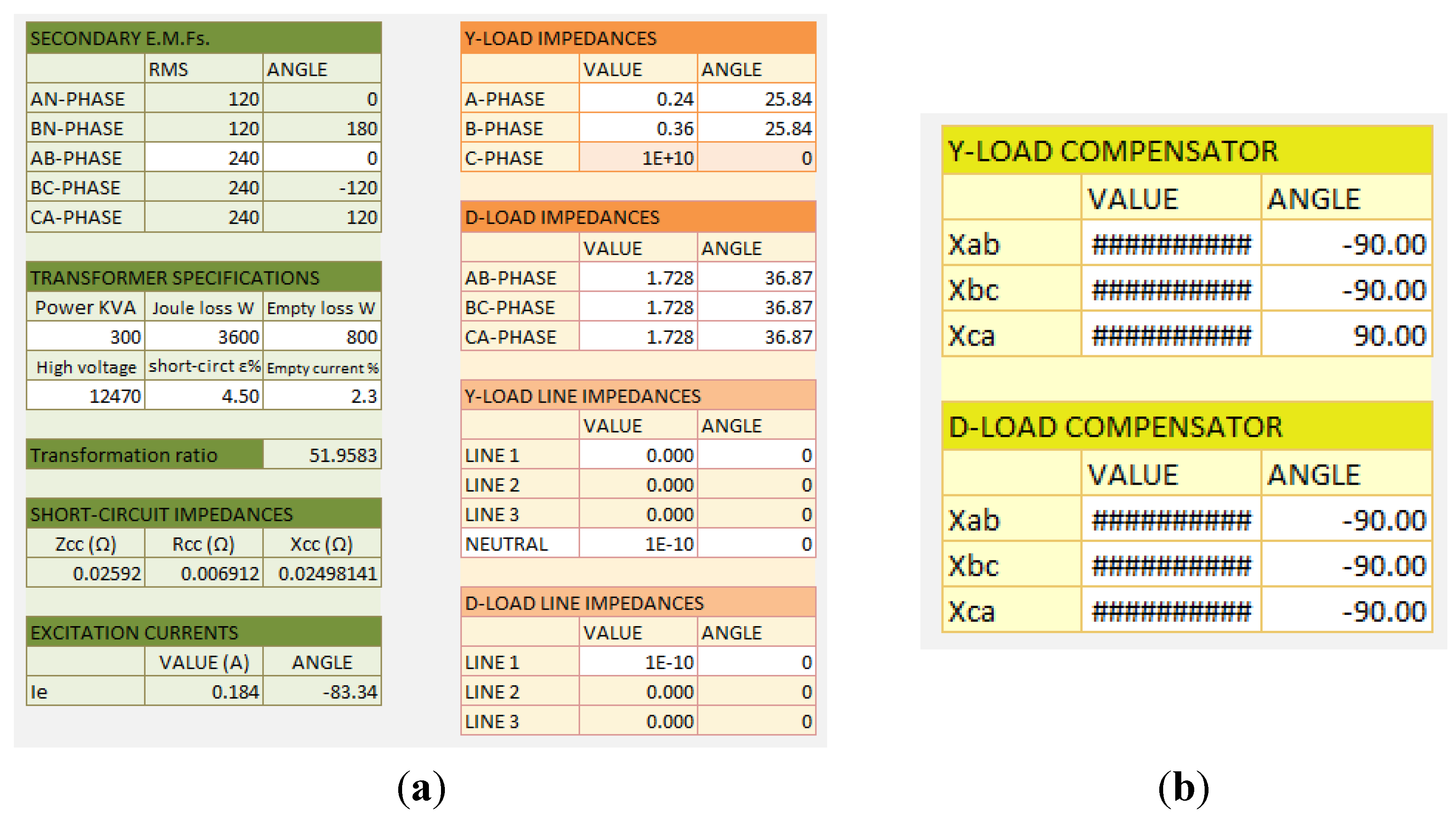
PF = 0.8), three-phase balanced delta load. The specifications of transformer and load impedances are shown in
Figure 5a, obtained from the simulator. The line impedances are considered negligible in this application example.
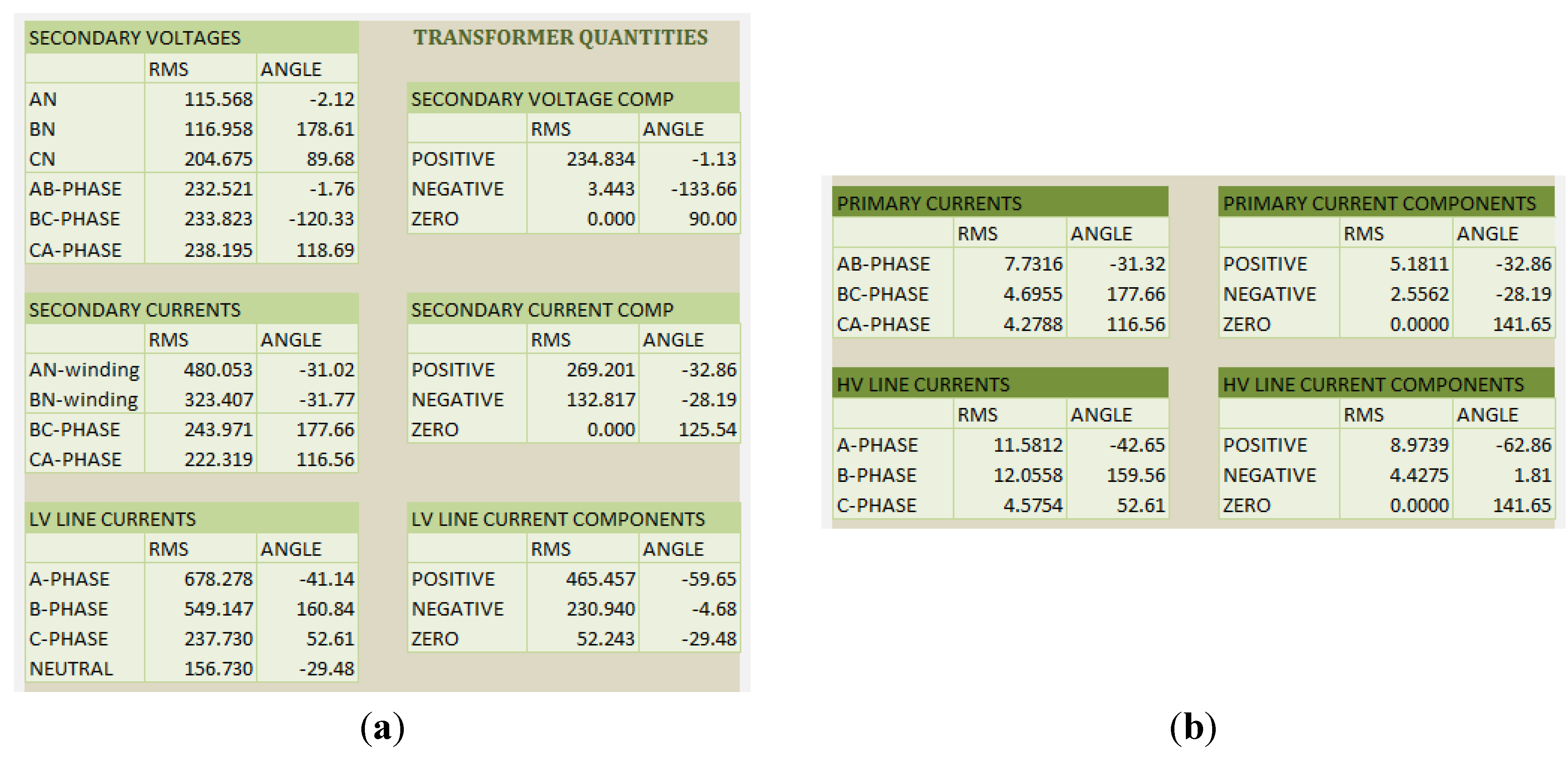
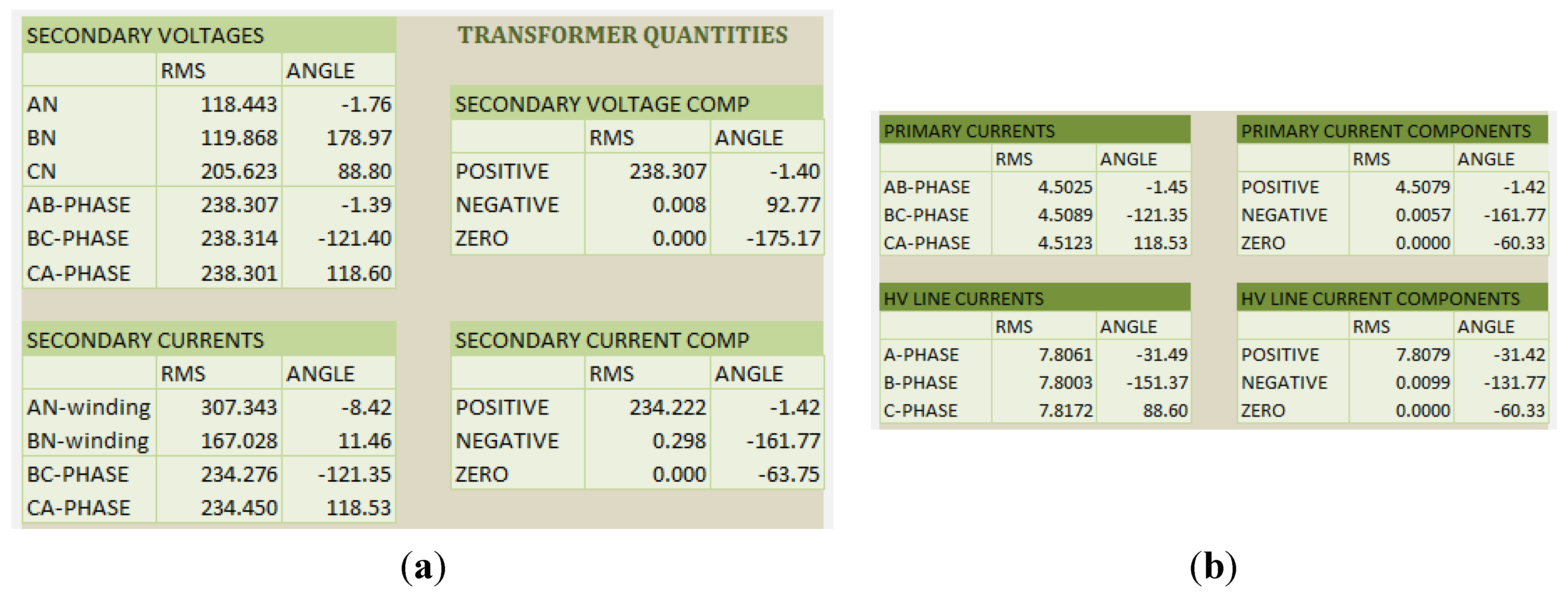
Voltages and currents in the secondary side (windings and lines) of the 4WD transformer can be seen in
Figure 6a, and the currents in the primary side (windings and lines) are included in
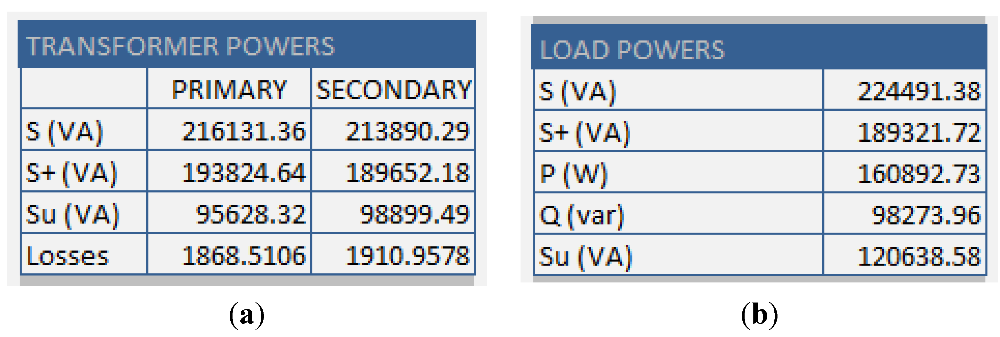
Figure 6b. Great current imbalances are observed in the primary and secondary sides of the transformer when it supplies those loads, but the primary currents are less unbalanced than in the secondary, because the zero-sequence currents have been filtered in the primary; then, the impact of the secondary neutral currents on the HV mains are cancelled out with this service. This fact is noticed from the apparent and unbalanced powers, whose values are less in the primary than in the secondary (
Figure 7a). It is noted that the load is more unbalanced than the source (transformer) due to the high voltage imbalance in the wye load (
Figure 7b).
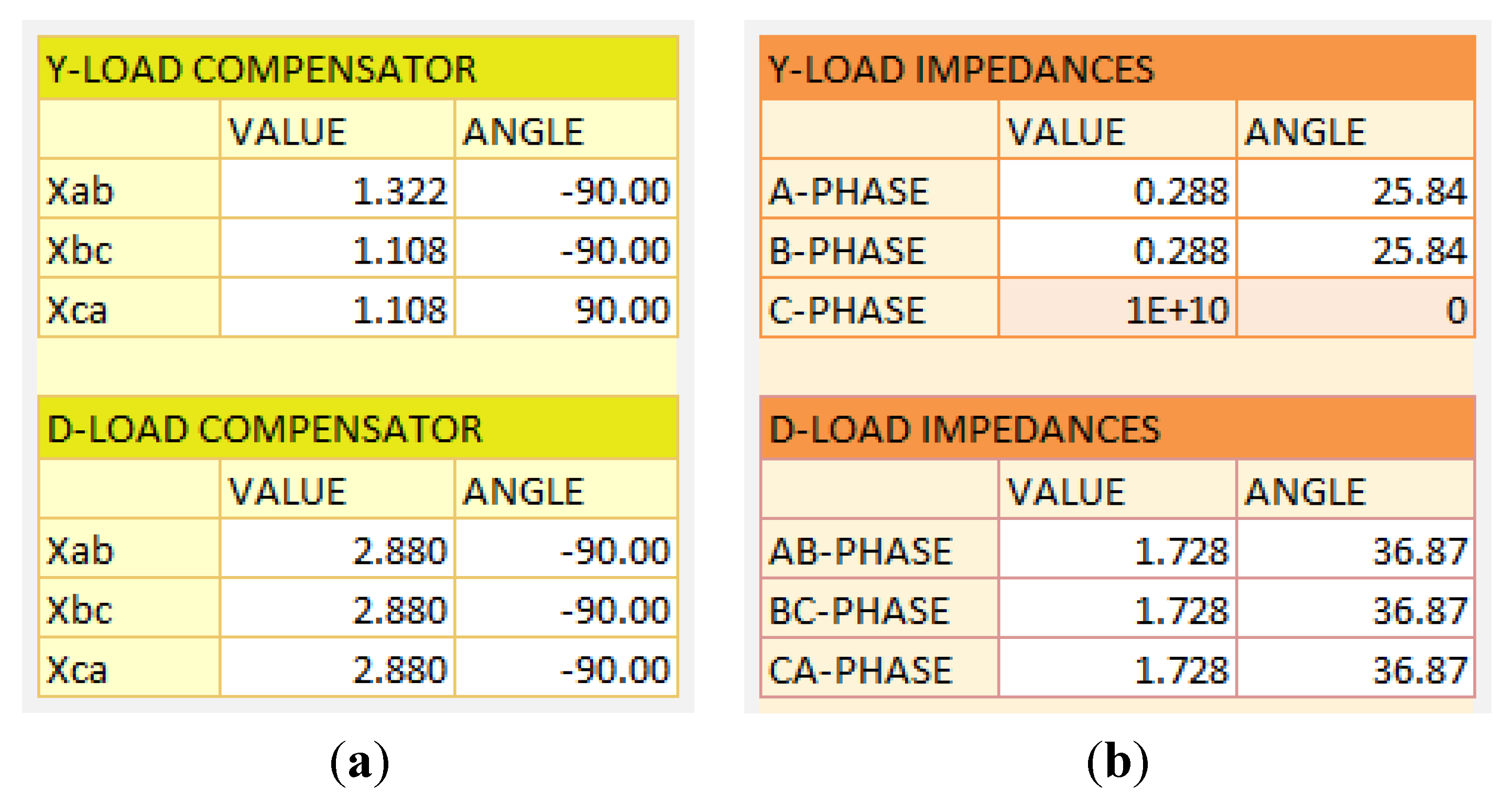
Figure 5.
(a) Transformer, line and load specifications; (b) compensator insertion data area.
Figure 5.
(a) Transformer, line and load specifications; (b) compensator insertion data area.
Figure 6.
4WD transformer voltages and currents: (a) secondary side; (b) primary side.
Figure 6.
4WD transformer voltages and currents: (a) secondary side; (b) primary side.
Figure 7.
(a) Transformer powers and losses; (b) load powers.
Figure 7.
(a) Transformer powers and losses; (b) load powers.
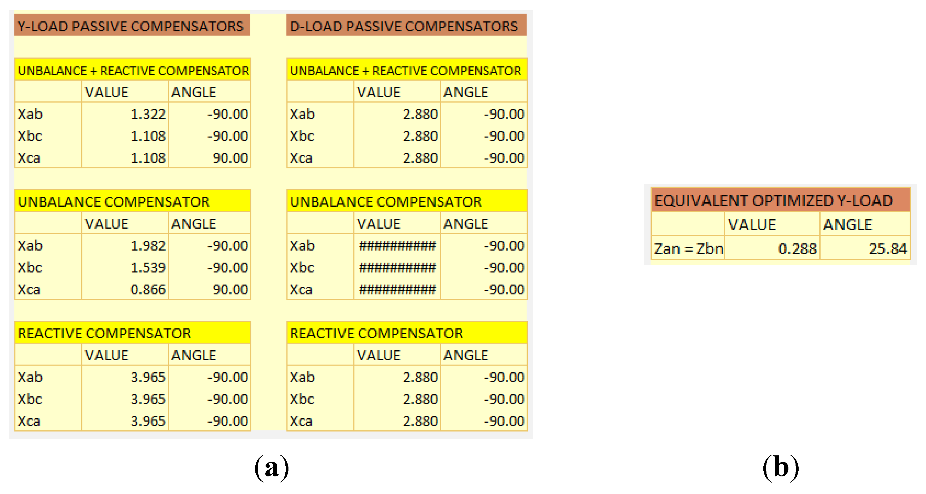
Once the load specifications are inserted in their respective boxes, the simulator determines the values of the necessary compensation devices (reactive, unbalanced or integral) for each load (
Figure 8a), as well as the optimized wye load that cancels the neutral current (
Figure 8b).
Figure 8.
Compensation devices and techniques: (a) passive compensators; (b) optimized wye load.
Figure 8.
Compensation devices and techniques: (a) passive compensators; (b) optimized wye load.
Those passive compensator elements for each load can be inserted in the compensator boxes (
Figure 5b) or not. In the first case, the effects of the compensation could be evaluated. The second case is to analyze the actual 4WD service operation without compensating. In the same way, the impedances of the equivalent optimized wye load (
Figure 8b) could be inserted in the wye impedances box of
Figure 5a instead of the actual wye load impedances, in order to evaluate the effects of the single-phase load distribution.
By selecting the compensation devices from the
Figure 8a, e.g., the integral compensator (reactive + unbalanced) for compensating the wye load and the reactive compensator for the delta load, and inserting those values in the boxes of
Figure 5b, a set of elements as is indicated in
Figure 9a could be obtained. The new voltages and currents in the transformer when those compensators were connected are those presented in
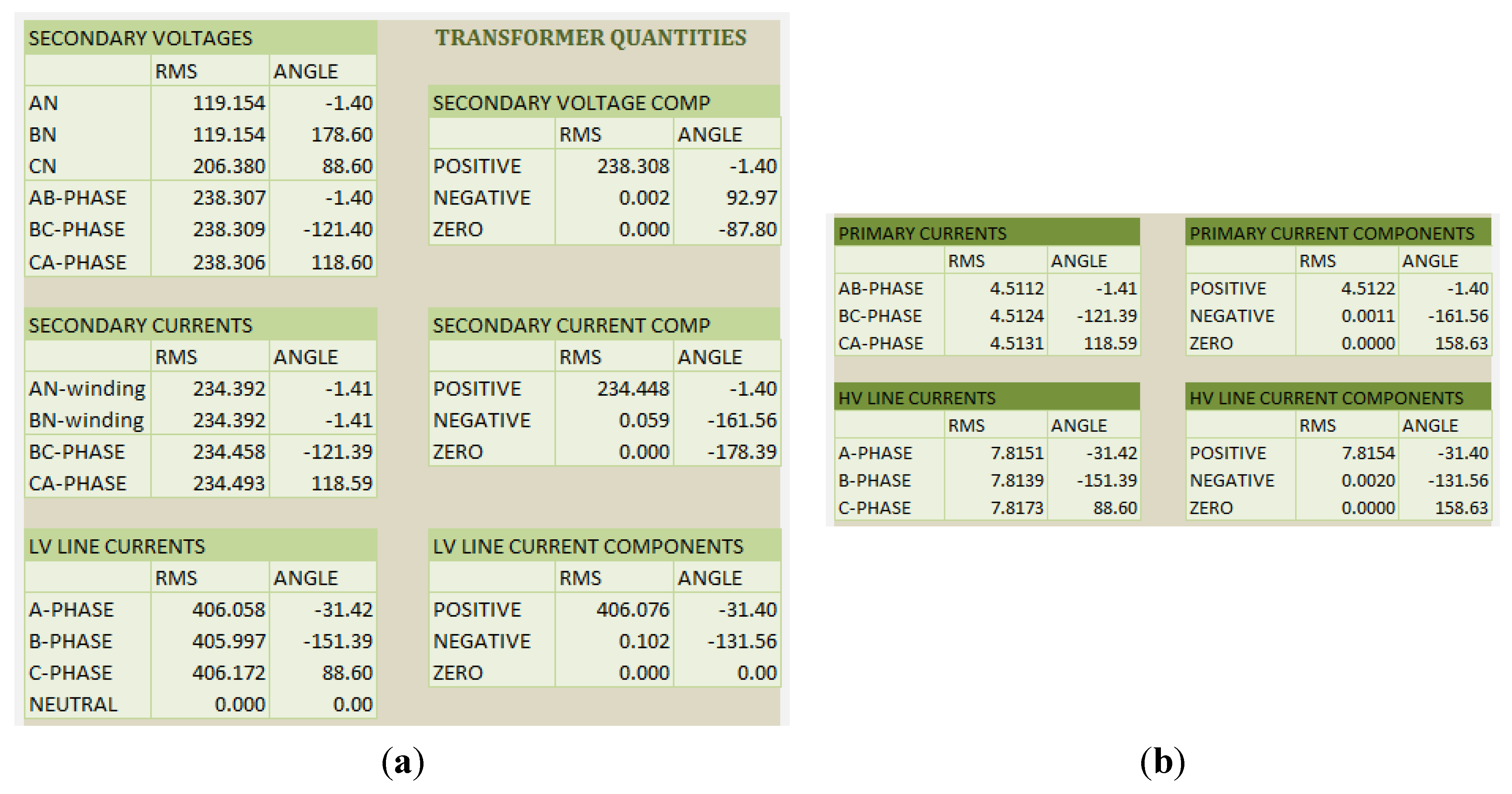
Figure 10a and b. Comparing
Figure 6 and
Figure 10, it is noted the negative-sequence voltages and currents in the transformer are strongly decreased after the compensation; the currents in the primary and in the HV mains are practically balanced, with positive-sequence (
Figure 10b).
Figure 9.
Selection of: (a) the compensation devices, (b) the optimal distributed wye load.
Figure 9.
Selection of: (a) the compensation devices, (b) the optimal distributed wye load.
Figure 10.
4WD transformer voltages and currents after compensation: (a) secondary side; (b) primary side.
Figure 10.
4WD transformer voltages and currents after compensation: (a) secondary side; (b) primary side.
It is observed from
Figure 10b and
Figure 11b that the currents in the primary side (windings and lines) are almost unaffected by the wye load distribution, since they practically remain balanced after the load compensation; thus, if our main interest is to look after the HV mains, it is not necessary to apply wye load distribution tasks. However, the transformer operation could be affected by the wye load distribution. Indeed, the currents in the secondary windings and in the LV lines are not fully rectified after compensation (
Figure 10a), but they remain minimized and balanced after the wye load distribution (
Figure 11a).
This fact could be noted comparing the transformer powers after the load compensation in two situations: first, the wye loads are not equitably distributed (
Figure 12a) and, second, optimal distribution of the wye load (
Figure 12b). The primary apparent power is minimized in both situations, but the secondary apparent power is minimized only in the second case, where the unbalanced power is fully compensated. In the last situation, the power losses measured from the primary and secondary have the same values.
Figure 11.
4WD transformer voltages and currents after compensating and distributing the loads: (a) secondary side; (b) primary side.
Figure 11.
4WD transformer voltages and currents after compensating and distributing the loads: (a) secondary side; (b) primary side.
Figure 12.
Transformer powers: (a) not distributed the wye load; (b) optimal wye load distribution.
Figure 12.
Transformer powers: (a) not distributed the wye load; (b) optimal wye load distribution.
8. Conclusions
An off-line simulator based on Excel used for the evaluation and compensation of 4WD services in sinusoidal steady-state conditions has been described in the above sections. The simulator provides the values of voltages and currents in all aspects of that service after the specifications of the transformer, lines and loads are inserted. These voltages and currents are obtained according to equations derived from the first and second Kirchhoff’s Laws. Apparent powers and powers losses are determined by the simulator too. The transformer apparent powers and power losses are separately measured from the primary and secondary sides. Transformer apparent powers have been formulated at the primary and secondary windings according to Buchholz’s or UPM approaches and, then, transformer apparent powers and power losses maintain a certain proportionality. However, the secondary apparent powers are calculated from an original formulation that uses the LV line currents instead of the secondary winding currents; this constitutes a remarkable contribution of this paper, because the measurement of the LV line currents is easier than the transformer internal currents in practice. Primary and secondary power differences are caused by the secondary neutral current effects.
Another original formulation has been used to determine the load apparent power. Because the voltages applied to the wye and delta loads have very different degrees of imbalance (line to neutral voltages are strongly unbalanced, but the line to line voltages are shortly unbalanced), the load apparent power has been formulated in vector notation as the sum of the UPM vector apparent powers of the wye and delta loads, such as it was described in
Section 5.2. This formulation of the apparent power in vector notation had not been described in the technical literature until now.
The simulator provides the elements of the delta passive reactive and imbalance compensation devices, as well as the optimal wye load that minimizes the neutral current. The values of those passive elements can be included in specific boxes of the simulator in order to evaluate each of the compensation effects. The compensation devices minimize the reactive and the negative-sequence currents in the 4WD service, while the wye load distribution cancels out the zero-sequence currents. The wye load compensator could be built considering the reactive and negative line currents as those loads are the same as those created by a single-phase load of ¼ the parallel impedance of the wye loads and connected to a, b phases.
Because the secondary neutral currents do not affect the transformer primary currents, the connection of only the delta compensators to compensate the load negative-sequence line currents is enough to optimize the HV mains.
The Excel-based off-line simulator, such as it has been described in the paper, is limited to evaluating the sinusoidal steady-state operation of 4WD services, as well as the reactive and unbalanced power compensation. Whether the non-sinusoidal steady-state and transitory operations were necessary, e.g., either to determine the non-fundamental power or to analyze the impact on the connection and disconnection of the compensators, the FFT should be used in the analysis.


 ,
, 


