Online Estimation of Model Parameters and State of Charge of LiFePO₄ Batteries Using a Novel Open-Circuit Voltage at Various Ambient Temperatures

Abstract

This study describes an online estimation of the model parameters and state of charge (SOC) of lithium iron phosphate batteries in electric vehicles. A widely used SOC estimator is based on the dynamic battery model with predeterminate parameters. However, model parameter variances that follow with their varied operation temperatures can result in errors in estimating battery SOC. To address this problem, a battery online parameter estimator is presented based on an equivalent circuit model using an adaptive joint extended Kalman filter algorithm. Simulations based on actual data are established to verify accuracy and stability in the regression of model parameters. Experiments are also performed to prove that the proposed estimator exhibits good reliability and adaptability under different loading profiles with various temperatures. In addition, open-circuit voltage (OCV) is used to estimate SOC in the proposed algorithm. However, the OCV based on the proposed online identification includes a part of concentration polarization and hysteresis, which is defined as parametric identification-based OCV (OCV_PI). Considering the temperature factor, a novel OCV–SOC relationship map is established by using OCV_PI under various temperatures. Finally, a validating experiment is conducted based on the consecutive loading profiles. Results indicate that our method is effective and adaptable when a battery operates at different ambient temperatures.

1. Introduction

Rechargeable lithium-ion (Li-ion) batteries have recently become attractive for applications in electric vehicles (EVs) because of their high energy density, high power density, long cycle life, and low self-discharge [1]. Battery cells are connected in series and parallel to satisfy the requirements of high-power applications for EVs because of the insufficient voltage and capacity of a single cell. To maintain optimum battery performance and avoid potential safety hazards, the battery management system (BMS) has become an essential part of a battery pack. The most important function of the BMS is to estimate state of charge (SOC), which is provided to drivers to show remaining mileage, improve power distribution efficiency, and extend the expected life span of batteries [2,3]. However, a major disadvantage of the lithium iron phosphate (LiFePO₄) battery is its poor low-temperature performance that is mainly attributed to its intrinsic low electronic conductivity [4] and the slow diffusion of Li ions [5,6], which make accurate modeling of the dynamic behavior of the battery difficult. Consequently, accurately estimating SOC remains challenging and problematic under a wide ambient temperature range.

A wide variety of techniques have been proposed to estimate SOC, and each one has its relative merits. According to literature [7,8,9,10,11,12,13,14,15,16,17,18,19,20,21,22,23,24], we divide the most commonly used methods into two major categories according to the selected battery model, i.e., black box- and state-space-model-based on SOC estimation methods. These two types of methods are described as follows.

Black box-model-based methods, including those based on artificial neural networks, fuzzy logic optimization, and support vector machines (SVMs), have been used to estimate SOC online. Kang et al. [7] presented a new radial basis function neural network model to eliminate the degradation effect of a battery on the SOC estimation accuracy of the original trained model. Feng et al. [8] proposed a fuzzy logic method to estimate the dynamic SOC of lead acid battery online. Juan et al. [9] employed SVMs to estimate the SOC of a high-capacity LiFeMnPO₄ battery from an experimental data set. However, the good performance of these methods depends strongly on previously measured training data at selected operating conditions and the suitable training method based on minimum fitting error. In addition, the model training process imposes a heavy computational load and requires a large data set. Consequently, the reliability and applicability of these SOC estimators are subject to challenge.

The methods based on the state-space model with nonlinear filtering algorithms can be further categorized into two types, namely, SOC- and open-circuit voltage (OCV)-based estimators, depending on the variables taken as the state vector. The Kalman filter (KF) technique is commonly selected for state-space estimation because of the advantages of its close-loop nature and capability to regulate estimation error range dynamically. In the SOC-based estimator, SOC that is directly taken as the state vector of the KF algorithm has been widely studied in literature [10,11,12,13,14,15,16,17,18,19]. Plett is among the pioneers and representatives who used the KF algorithm to estimate the state vector of a battery state-space model. In his three-paper series [10,11,12], the extended KF (EKF) was applied to estimate the SOC of Li-ion polymer battery (LiPB) based on various battery models. Subsequently, Plett proposed the sigma-point KF, which outperforms EKF in nonlinear estimation applications, to estimate the SOC of LiPB in the latter two papers [13,14]. In addition, other nonlinear KF techniques, such as unscented KF [15,16], particle filter (PF) [17], and unscented PF [18], are widely used to estimate SOC. However, the performance of the SOC-based algorithm has two major flaws. First, the variables of system noise, such as mean value as well as relevance and covariance matrices, should be known in advance. Second, this method strongly depends on the precision of the battery model. Xiong et al. [19] used an adaptive EKF (AEKF)-based method to estimate SOC online. This technique improves estimation accuracy by adaptively updating the process and measurement noise covariance. Xing et al. [20] considered the temperature dependence of the relationship between OCV and SOC and presented an SOC estimation method based on a temperature model incorporated with an OCV–SOC–temperature table. However, the accuracy of this model at low temperature is obviously less than that at high temperature because battery model parameters are identified with off-line data. The different operating conditions that result in model parameter variances are ignored. In addition, the large error is partially caused by applying the simplified Rint model, which exhibits poor performance at low temperature because of the omission of the relaxation effect.

To overcome the second flaw of SOC-based algorithms, online parameter identification methods have been proposed to update model parameters in real time. OCV-based estimators achieve SOC inference by using the intrinsic relationship of a battery between SOC and some model parameters such as OCV. Xiong et al. [21,22] employed the AEKF algorithm to estimate model parameters and infer SOC. Plett and Pei et al. [12,23] proposed the dual EKF algorithm to conduct a training-free battery parameter/state estimation based on an equivalent circuit model. A common drawback of the aforementioned methods is the omission of cell parameter variances under different temperatures. The methods have also been verified under a narrow set of scenarios without considering different temperatures and loading profiles. The conventional relationship of OCV–SOC is frequently established at room temperature [24,25]. However, the relationship varies with differences in temperature and presents various results when a battery is operating at other ambient temperatures. In addition, the effects of overpotential and hysteresis are generally ignored during the process of establishing the relationship. The aforementioned factors lead to remarkable errors in inferring SOC under various temperatures.

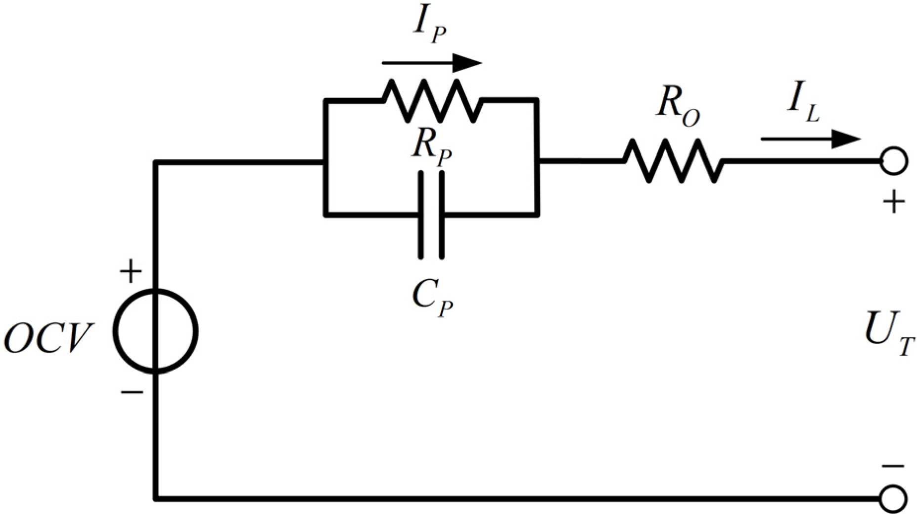
This study presents an SOC estimator for Li-ion batteries. The estimator is based on an adaptive online identification of its OCV according to a novel relationship map of OCV_PI–SOC–temperature (OCV_PI–SOC–T) for application in EVs under various temperatures. This paper is organized as follows. Section 2 describes the structure and discrete state-space formulation of the selected equivalent circuit battery model. 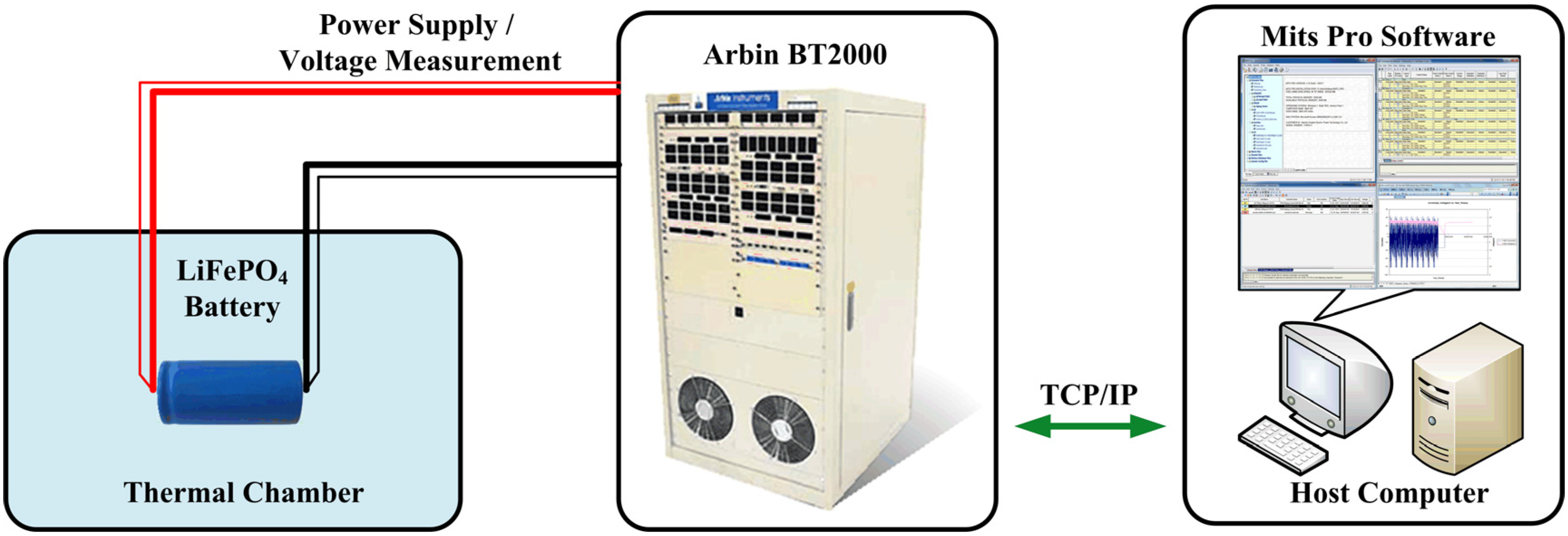In Section 3, the implementation flowchart of the online parameter identification method is proposed based on the review of the adaptive joint EKF (AJEKF). To verify the proposed approach, a 3.3 V/5 Ah LiFePO₄/graphite battery is used to execute a series of characteristic tests. The experiment procedure is described in Section 4. The simulations and experiments are discussed in Section 5 to validate the accuracy and reliability of the proposed method on estimating battery parameters. In Section 6, SOC estimation is conducted according to the OCV_PI–SOC–T map, and effectiveness and adaptability are validated and compared with conventional estimation methods that use OCV_VR–SOC–T and OCV_GT–SOC–T maps. Finally, Section 7 concludes the paper.

2. Modeling LiFePO₄ Batteries

To achieve reliable battery parameter identification, a suitable battery model should be constructed first. Afterward, to estimate the parameters and state of a system based on AJEFK, a discrete state-space equation for the battery model should be available.

2.1. Selecting the Model

In [26], several kinds of battery models used to characterize battery electrochemical behavior were introduced and evaluated. To achieve good balance between response speed and computational power, a first-order resistance–capacitance (RC) circuit model is selected as the object for identifying model parameters in this study. As shown in Figure 1, the model comprises an OCV, a resistance (R_O), as well as parallel resistance and capacitance (R_PC_P) connected in series.

Figure 1. First-order resistance–capacitance (RC) circuit model.

Figure 1. First-order resistance–capacitance (RC) circuit model.

In the model, I_L indicates the load current (positive for discharge, negative for charge) and U_T denotes terminal voltage. OCV is used to express the internal voltage source of the battery model. Ro (i.e., ohmic resistance) represents the bulk resistance of the cell, which reflects the electrical conductivity of the electrolyte, the separator, and the electrodes. Rp and Cp (i.e., activation polarization resistance and activation polarization capacitance, respectively) are the lumped interfacial resistance and the electric double-layer capacitance, respectively, between the electrode and the electrolyte during activation polarization. I_P (i.e., activation polarization current) is the current that flows through R_P. The electrical behavior of the proposed model can be expressed by Equation (1):

$$\{\begin{array}{l}\frac{d{I}_P}{dt}=\frac{1}{R_P{C}_P}(I_L-I_P)\\ U_T=OCV-I_L\times R_o-I_p\times R_p\end{array}$$

(1)

2.2. Establishing the Discrete State-Space Equation

To implement the proposed approach for online parameters and state identification, we first performed a discretization process for the first-order RC circuit model, and then formulated regression equations for the discretization system. The regression equations were used as state-space equations, and discussed in the next section.

Assuming that a BMS has a reasonable sampling frequency in EV applications, then the model parameters vary slightly and load current remains constant between two adjacent measurement points k and k+1 (i.e., $d{I}_L/dt=0$, in the period t_k to t_k+1). During one sampling period, we obtained the Laplace transform on both sides of the first-order differential equation in Equation (1), as follows:

$$s{I}_P(s)-I_P(t_k)=\frac{1}{R_P{C}_P}(\frac{I_L}{s}-I_P(s))$$

(2)

where s is the Laplace operator. Afterward, Equation (2) can be rewritten as follows:

$$I_P(s)=\frac{I_P(t_k)}{s+\frac{1}{R_P{C}_P}}\text{+}\frac{\frac{1}{R_P{C}_P}{I}_L}{s(s+\frac{1}{R_P{C}_P})}$$

(3)

The activation polarization current I_P can be obtained by inverse Laplace transform as follows:

$$I_P(t_{k+1})=\exp (\frac{-\mathrm{\Delta }t}{R_P{C}_P})\times I_P(t_k)+(1-\text{exp}(\frac{-\mathrm{\Delta }t}{R_P{C}_P}))\times I_L$$

(4)

where $\mathrm{\Delta }t$ is the sampling period. To minimize the measurement error of the current sensor, load current I_L is substituted by the average value of two adjacent current sampling points during regression. The state-space equation of the battery model can be discretized as follows:

$$\{\begin{array}{l}{I}_{p,k+1}=\exp (\frac{-\mathrm{\Delta }t}{R_P{\mathrm{C}}_P})\times I_{p,k}+(1-\exp (\frac{-\mathrm{\Delta }t}{R_P{\mathrm{C}}_P}))\times (I_{L,k+1}+I_{L,k})/2\\ U_{T,k+1}=OCV-I_{L,k+1}\times R_o-I_{p,k+1}\times R_p\end{array}$$

(5)

where subscript k denotes the kth sampling point.

3. Online Estimation of Model Parameters

To guarantee the accurate online identification results of the state and the parameters of the battery model, a reasonable mathematical algorithm is necessary. Online identification suffers from strong nonlinearity, which can be observed from any battery model parameter that has a nonlinear relationship with SOC. In addition, uncertainties attributed to the predetermined variables of system noise, such as mean value, pertinence, and covariance matrix, result in remarkable errors and divergence. The adaptive nonlinear filtering algorithm based on the selected model was developed by exploiting KF and adapted to concurrently estimate both state and parameters. Thus, the AJEKF algorithm was chosen, which can provide an effective means to estimate the state and parameters of a system simultaneously.

3.1. AJEKF Algorithm

KF is a mathematical technique that provides an efficient recursive means to estimate the states of a process to minimize the mean squared error [10]. Given that KF is only available for linear systems, EKF uses a linearization process at each time step to approximate a nonlinear system through the first-order Taylor series expansion [19].

The JEKF method, which is based on EKF, was presented by Wan et al. in 2001 [27]. This algorithm augments the state vector of a system with its parameters and uses EKF on an augmented system with large matrix operations. The filter has been applied extensively to estimate both state and parameters. The dynamics of the state and parameters within a joint filter are combined to create an augmented system as follows:

$$\left[\begin{array}{c}{x}_{k+1}\\ {\theta }_{k+1}\end{array}\right]=\left[\begin{array}{c}f(x_k,u_k,{\theta }_k)\\ {\theta }_k\end{array}\right]+\left[\begin{array}{c}{w}_k\\ r_k\end{array}\right]$$

(6)

$$y_k=g(x_k,u_k,{\theta }_k)+v_k$$

(7)

where ${\theta }_k$ denotes the parameters that are essentially constant, but may change slowly over time by some driving processes, modeled by a process $r_k$ of a small fictitious “noise”. To simplify notation, we refer to the vector that comprises the present state and parameters as ${\chi }_k$ and the equation that combines the dynamics of the state and parameters as $ℱ$. The discrete-time state-space equations are rewritten as follows:

$$X_{k+1}=ℱ({\chi }_k,u_k)+\left[\begin{array}{c}{w}_k\\ r_k\end{array}\right]$$

(8)

$$y_k=g({\chi }_k,u_k)+v_k$$

(9)

Given that the augmented model of the system and the parameter dynamics are defined, we apply the EKF method. However, a drawback of this method is that the covariances of the process and the measurement noise should be known in advance. In practice, this approach fails to ensure its performance if the initial noise information is inappropriate. Thus, the application of an AJEKF that employs the covariance matching approach to realize robust online identification is discussed in this section.

AJEKF adds further innovation to the algorithm by using the innovation sequence of the filter. The innovation allows parameters $Q_{v,k}$ and $diag(Q_{w,k+1},Q_{r,k+1})$ to be estimated and updated iteratively from the following equations [28]:

$$H_k=\frac{1}{M}{\displaystyle {\sum }_{i=k-M+1}^k{e}_k{e}_k^T}$$

(10)

$$\{\begin{array}{l}{Q}_{v,k}=H_k-C_k{P}_{\tilde{X},k}^{-}{C}_k^T\\ diag(Q_{w,k+1},Q_{r,k+1})=K_k{H}_k{K}_k^T\end{array}$$

(11)

where $H_k$ is the innovation covariance matrix based on the innovation sequence $e_k$ within a moving estimation window with size $M$.

The calculation steps of the AJEKF algorithm are shown in Table 1, where $K_k$ is the Kalman gain matrix; $e_i$ is defined as the difference between observation $y_k$ and predicted observation $g({\hat{\chi }}_k^{-},u_k)$; $\hat{{\displaystyle }}$ represents an estimation value; and ${\stackrel{ˆ}{}}^{-}$ and ${\stackrel{ˆ}{}}^{+}$ represent prior and posteriori estimation values, respectively. The rest of the steps are similar to those of the standard EKF, but with larger matrix operations.

Table 1. Summary of AJEKF for estimating state and parameters.

	Nonlinear state-space models a:
	$\left[\begin{array}{c}{x}_{k+1}\\ {\theta }_{k+1}\end{array}\right]=\left[\begin{array}{c}f(x_k,u_k,{\theta }_k)\\ {\theta }_k\end{array}\right]+\left[\begin{array}{c}{w}_k\\ r_k\end{array}\right]$ or $X_{k+1}=ℱ({\chi }_k,u_k)+\left[\begin{array}{c}{w}_k\\ r_k\end{array}\right]$
	$y_k=g(x_k,u_k,{\theta }_k)+v_k$ $y_k=g({\chi }_k,u_k)+v_k$
	Definitions:
	$A_{k-1}={\frac{\partial ℱ({\chi }_{k-1},u_{k-1})}{\partial {\chi }_{k-1}}|}_{{\chi }_{k-1}={\hat{\chi }}_{k-1}^{+}}$ $C_k={\frac{\partial g({\chi }_k,u_k)}{\partial {\chi }_k}|}_{{\chi }_k={\hat{\chi }}_k^{-}}$
	Initialization:
	For k = 0, set
	${\hat{\chi }}_0^{+}=E[X_0]$
	$P_{\tilde{\chi }}^{+}=E[({\chi }_0-{\hat{\chi }}_0^{+}){({\chi }_0-{\hat{\chi }}_0^{+})}^T]$
	Computation:
	For k = 1, 2, …; compute:
	State estimation time update: ${\hat{\chi }}_k^{-}=ℱ({\hat{\chi }}_{k-1}^{+},u_{k-1})$
	Error innovation: $e_k=y_k-g({\hat{\chi }}_k^{-},u_k)$
	Error covariance time update: $P_{\tilde{\chi },k}^{-}=A_{k-1}{P}_{\tilde{\chi },k-1}^{+}{A}_{k-1}^T+diag(Q_{w,k},Q_{r,k})$
	Adaptive law-covariance matching:
	$H_k=\frac{1}{M}{\displaystyle {\sum }_{i=k-M+1}^k{e}_k{e}_k^T}$, $Q_{v,k}=H_k-C_k{P}_{\tilde{\chi },k}^{-}{C}_k^T$
	Kalman gain matrix: $K_k=P_{\tilde{\chi },k}^{-}{C}_k^T[C_k{P}_{\tilde{\chi },k}^{-}{C}_k^T+Q_{v,k}]$
	State estimation measurement update: ${\hat{\chi }}_k^{+}={\hat{\chi }}_k^{-}+K_k{e}_k$
	Noise and error covariance measurement update:
	$diag(Q_{w,k+1},Q_{r,k+1})=K_k{H}_k{K}_k^T$, $P_{\tilde{\chi },k}^{+}=(I-K_k{C}_k)P_{\tilde{\chi },k}^{-}$

^a $w_k$, $v_k$, and $r_k$ are the independent, zero-mean, and Gaussian noise processes of covariance matrices $Q_w$, $Q_v$, and $Q_r$, respectively.

Table 1. Summary of AJEKF for estimating state and parameters.

	Nonlinear state-space models a:
	$\left[\begin{array}{c}{x}_{k+1}\\ {\theta }_{k+1}\end{array}\right]=\left[\begin{array}{c}f(x_k,u_k,{\theta }_k)\\ {\theta }_k\end{array}\right]+\left[\begin{array}{c}{w}_k\\ r_k\end{array}\right]$ or $X_{k+1}=ℱ({\chi }_k,u_k)+\left[\begin{array}{c}{w}_k\\ r_k\end{array}\right]$
	$y_k=g(x_k,u_k,{\theta }_k)+v_k$ $y_k=g({\chi }_k,u_k)+v_k$
	Definitions:
	$A_{k-1}={\frac{\partial ℱ({\chi }_{k-1},u_{k-1})}{\partial {\chi }_{k-1}}|}_{{\chi }_{k-1}={\hat{\chi }}_{k-1}^{+}}$ $C_k={\frac{\partial g({\chi }_k,u_k)}{\partial {\chi }_k}|}_{{\chi }_k={\hat{\chi }}_k^{-}}$
	Initialization:
	For k = 0, set
	${\hat{\chi }}_0^{+}=E[X_0]$
	$P_{\tilde{\chi }}^{+}=E[({\chi }_0-{\hat{\chi }}_0^{+}){({\chi }_0-{\hat{\chi }}_0^{+})}^T]$
	Computation:
	For k = 1, 2, …; compute:
	State estimation time update: ${\hat{\chi }}_k^{-}=ℱ({\hat{\chi }}_{k-1}^{+},u_{k-1})$
	Error innovation: $e_k=y_k-g({\hat{\chi }}_k^{-},u_k)$
	Error covariance time update: $P_{\tilde{\chi },k}^{-}=A_{k-1}{P}_{\tilde{\chi },k-1}^{+}{A}_{k-1}^T+diag(Q_{w,k},Q_{r,k})$
	Adaptive law-covariance matching:
	$H_k=\frac{1}{M}{\displaystyle {\sum }_{i=k-M+1}^k{e}_k{e}_k^T}$, $Q_{v,k}=H_k-C_k{P}_{\tilde{\chi },k}^{-}{C}_k^T$
	Kalman gain matrix: $K_k=P_{\tilde{\chi },k}^{-}{C}_k^T[C_k{P}_{\tilde{\chi },k}^{-}{C}_k^T+Q_{v,k}]$
	State estimation measurement update: ${\hat{\chi }}_k^{+}={\hat{\chi }}_k^{-}+K_k{e}_k$
	Noise and error covariance measurement update:
	$diag(Q_{w,k+1},Q_{r,k+1})=K_k{H}_k{K}_k^T$, $P_{\tilde{\chi },k}^{+}=(I-K_k{C}_k)P_{\tilde{\chi },k}^{-}$

^a $w_k$, $v_k$, and $r_k$ are the independent, zero-mean, and Gaussian noise processes of covariance matrices $Q_w$, $Q_v$, and $Q_r$, respectively.

3.2. Implementing AJEKF on the Battery Model

To estimate the state and parameters of the battery model in the AJEKF framework, state and parameter vectors must be confirmed in the algorithm. The activation polarization current I_P, which depends on both previous short-time information and the present input, is taken as the state vector. All parameters in the battery model, which may not be directly determined through knowledge of the measured input/output of the system and have a slow rate of change, are taken as the parameter vector of the system. State vector $x$ and parameter vector $\theta$ are defined as follows:

$$x=I_p$$

(12)

$$\theta ={[\begin{array}{cccc}OCV& R_O& R_P& C_P\end{array}]}^T$$

(13)

Terminal voltage $U_T$ is selected as the measured system output, and $y=U_T$. Battery load current $I_L$ can be regarded as exogenous input $u$.

The state-space equation can be expressed as follows:

$$X_{k+1}=\left(\begin{array}{c}{x}_{k+1}\\ \\ {\theta }_{k+1}\\ \\ \end{array}\right)=\left(\begin{array}{c}{I}_{P,k+1}\\ OC{V}_{k+1}\\ R_{O,k+1}\\ R_{P,k+1}\\ C_{P,k+1}\end{array}\right)=\left(\begin{array}{c}\exp (-\mathrm{\Delta }t/(R_{P,k}{C}_{P,k}))I_{P,k}+(1-\exp (-\mathrm{\Delta }t/(R_{P,k}{C}_{P,k})))(I_{L,k+1}+I_{L,k})/2\\ OC{V}_k\\ R_{O,k}\\ R_{P,k}\\ C_{P,k}\end{array}\right)+\left(\begin{array}{c}{w}_k\\ \\ r_k\\ \\ \end{array}\right)$$

(14)

In addition, $U_T$ consists of the OCV, ohmic voltage, and activation polarization voltage. The system measurement equation is as follows:

$$y_k=g(X_k,u_k)+v_k=OC{V}_k-I_{L,k}{R}_{O,k}-I_{P,k}{R}_{P,k}+v_k$$

(15)

Each time step $A_{k-1}$ and $C_k$, which are respectively the derivation matrices of $ℱ({\chi }_{k-1},u_{k-1})$ and $g({\chi }_k,u_k)$ with respect to system state vector ${\chi }_k$, are calculated as follows:

$$\begin{array}{ll}{A}_{k-1}& ={\frac{\partial ℱ({\chi }_{k-1},u_{k-1})}{\partial {\chi }_{k-1}}|}_{{\chi }_{k-1}={\hat{\chi }}_{k-1}^{+}}\\ & =\left[\begin{array}{cc}\frac{\partial f(x_{k-1},u_{k-1},{\theta }_{k-1})}{\partial x_{k-1}}& \frac{\partial f(x_{k-1},u_{k-1},{\theta }_{k-1})}{\partial {\theta }_{k-1}}\\ \frac{\partial {\theta }_{k-1}}{\partial x_{k-1}}& \frac{\partial {\theta }_{k-1}}{\partial {\theta }_{k-1}}\end{array}\right]\\ & =\left[\begin{array}{ccccc}\exp (\frac{-\mathrm{\Delta }t}{{\hat{R}}_{P,k-1}^{+}{\hat{C}}_{P,k-1}^{+}})& 0& 0& \begin{array}{l}\exp (\frac{-\mathrm{\Delta }t}{{\hat{R}}_{P,k-1}^{+}{\hat{C}}_{P,k-1}^{+}})\frac{\mathrm{\Delta }t}{{({\hat{R}}_{P,k-1}^{+})}^2{\hat{C}}_{P,k-1}^{+}}{I}_{P,k-1}\\ -\exp (\frac{-\mathrm{\Delta }t}{{\hat{R}}_{P,k-1}^{+}{\hat{C}}_{P,k-1}^{+}})\frac{\mathrm{\Delta }t}{{({\hat{R}}_{P,k-1}^{+})}^2{\hat{C}}_{P,k-1}^{+}}(\frac{I_{L,k-1}+I_{L,k-2}}{2})\end{array}& \begin{array}{l}\exp (\frac{-\mathrm{\Delta }t}{{\hat{R}}_{P,k-1}^{+}{\hat{C}}_{P,k-1}^{+}})\frac{\mathrm{\Delta }t}{{\hat{R}}_{P,k-1}^{+}{({\hat{C}}_{P,k-1}^{+})}^2}{I}_{P,k-1}\\ -\exp (\frac{-\mathrm{\Delta }t}{{\hat{R}}_{P,k-1}^{+}{\hat{C}}_{P,k-1}^{+}})\frac{\mathrm{\Delta }t}{{\hat{R}}_{P,k-1}^{+}{({\hat{C}}_{P,k-1}^{+})}^2}(\frac{I_{L,k-1}+I_{L,k-2}}{2})\end{array}\\ 0& 1& 0& 0& 0\\ 0& 0& 1& 0& 0\\ 0& 0& 0& 1& 0\\ 0& 0& 0& 0& 1\end{array}\right]\end{array}$$

(16)

$$\begin{array}{ll}{C}_k=& {\frac{\partial g({\chi }_k,u_k)}{\partial {\chi }_k}|}_{{\chi }_k={\hat{\chi }}_k^{-}}\\ & =\left[\begin{array}{cc}\frac{\partial g(x_k,u_k,{\theta }_k)}{\partial x_k}& \frac{\partial g(x_k,u_k,{\theta }_k)}{\partial {\theta }_k}\end{array}\right]\\ & =\left[\begin{array}{ccccc}{\hat{R}}_{P,k}^{-}& 1& I_{L,k}& {\hat{I}}_{P,k}^{-}& {\hat{R}}_{P,k}^{-}(\exp (\frac{-\mathrm{\Delta }t}{{\hat{R}}_{P,k-1}^{+}{\hat{C}}_{P,k-1}^{+}})\frac{\mathrm{\Delta }t}{{\hat{R}}_{P,k-1}^{+}{({\hat{C}}_{P,k-1}^{+})}^2}{\hat{I}}_{P,k}^{-}-\exp (\frac{-\mathrm{\Delta }t}{{\hat{R}}_{P,k-1}^{+}{\hat{C}}_{P,k-1}^{+}})\frac{\mathrm{\Delta }t}{{\hat{R}}_{P,k-1}^{+}{({\hat{C}}_{P,k-1}^{+})}^2}(\frac{I_{L,k}+I_{L,k-1}}{2}))\end{array}\right]\end{array}$$

(17)

4. Battery Experiments

4.1. Experiment Setup

The test bench setup (Figure 2) consists of (1) rectangular Li-ion cells (LiFePO₄/graphite, nominal capacity: 5 Ah, upper/lower cutoff voltage: 3.65 V/2.5 V, and upper/lower pulse current: 10 A/−15 A); (2) a thermal test chamber for the environment, which has a temperature operation range between −55 °C and 150 °C; (3) a battery test system (the Arbin BT2000 tester has a maximum voltage of 5 V and a maximum charging/discharging current of ±200 A; the measurement inaccuracy of the current and voltage transducers within the Arbin BT2000 system is within 0.1%); and (4) a PC with Arbin’s Mits Pro Software for battery charging/discharging control. The Arbin BT2000 is connected to the battery cell, which is placed inside the thermal chamber to maintain temperature. The measured data are transmitted to the host computer through TCP/IP ports.

Figure 2. Schematic of the battery test bench.

Figure 2. Schematic of the battery test bench.

4.2. Experiment Procedure

The experiment procedure for our research is shown in Figure 3. The procedure was designed to collect cell test data under our designed program. A series of characterization tests (static capacity, coulombic efficiency, OCV–SOC, and loading profile tests) were conducted at five different temperatures (from 0 °C–40 °C at 10 °C interval). The data sheets and the test method for the characteristic test are described in detail in [29]; however, the nominal current is 1/3 C (1.67 A) for the experiment object. Two different simulation driving cycles, i.e., the federal urban driving schedule (FUDS) and the dynamic stress test (DST) loading profiles [30] were employed to verify and evaluate the performance of the parameter identification method (in Section 5) and the reliability of the proposed SOC estimator (in Section 6). The other characterization tests (expectations for the loading profiles) were conducted at a special temperature to obtain the SOC reference profiles in Section 6.

Figure 3. Battery experiment procedure.

Figure 3. Battery experiment procedure.

5. Results and Discussion

The proposed methods were applied to the aforementioned tests, and the results are discussed in this section. First, Section 5.1 provides an overview of the regression capability of the online parameter identification algorithm by using simulated data. In Section 5.2, the proposed adaptive online parameter estimator was verified by using DST and FUDS tests at different ambient temperatures.

5.1. Verifying the AJEKF Algorithm with Simulated Data

The previous section describes the AJEKF algorithm, including the formulas and procedures used for the online identification of battery parameters and state. This section presents a simulation experiment within a test environment that was employed along with simulated data to verify the regression accuracy of the identification algorithm. The simulated data and the verification procedure are as follows. First, model parameter values were prescribed and considered as the true values of the identification results. Then, voltage data U_T were determined based on the prescribed values of the parameters and I_L data. The values of I_L and U_T were used for real-time regression. Finally, the effectiveness and stability of the algorithm were assessed by comparing the regressed parameter values with the prescribed values.

To provide an example of the simulation tests, the model parameters were prescribed as OCV = 3.25 V, R_O = 20 mΩ, R_P = 15 mΩ, and C_P = 2000 F, which were taken as true values to validate the identification results. The simulated current data were synthesized by adding Gaussian white noise with the standard deviations of 5 mA to the current values of FUDS profiles at 40 °C. Based on the simulated current data and the selected parameters, the simulated voltage data were calculated using the circuit model. The sets of simulated values of U_T and I_L are shown in Figure 4. Then, U_T and I_L data were inputted into the algorithm to obtain the identification values of the model parameters. The initial values of the parameters were set as OCV = 3 V, R_O = 10 mΩ, R_P = 5 mΩ, and C_P = 1800 F.

Figure 4. Synthesized current data and deduced voltage data from the equivalent circuit model.

Figure 4. Synthesized current data and deduced voltage data from the equivalent circuit model.

The estimated parameters and their prescribed values are depicted in Figure 5, wherein the red and blue lines denote the prescribed and estimated values, respectively. The identification values of the parameters converged to the prescribed values and exhibited minimal variation over time, which attest to the accuracy and stability of the algorithm during parameter regression. Regression was very fast despite few deviations between the initial and prescribed values.

Figure 5. Regression of the estimated parameters based on simulated data: (a) OCV; (b) R_O; (c) R_P; and (d) C_P.

Figure 5. Regression of the estimated parameters based on simulated data: (a) OCV; (b) R_O; (c) R_P; and (d) C_P.

5.2. Verifying Model Parameter and State Estimator with Experimental Data

This section verifies and evaluates the identification of model parameters and state by using two loading profiles at five different temperatures. In Section 5.2.1 and Section 5.2.2, the proposed method was verified with DST and FUDS loading profiles, respectively.

5.2.1. DST Loading Profile Test

5.2.1.1. DST Experiment Data

DST was designed by the US Advanced Battery Consortium (USABC) to simulate a variable-power discharge regime that represents the expected demands of an EV battery [20]. A completed DST loading profile is 360 s long and can be scaled down to any desired power or current pulse demand according to the specifications of the battery samples. In our research, the DST test was performed with the current profiles and terminated when the cell reached the lower cutoff voltage. The measured current and voltage profiles at 40 °C are shown in Figure 6, in which the cell is fully charged with the nominal constant current and constant voltage (CCCV) method. Thus, the initial SOC started at 100%. The test profiles and time lengths were different under different ambient temperatures because of difference in capacities.

Figure 6. DST loading profiles at 40 °C: (a) voltage and current vs. time profiles and (b) enlarged version of (a).

Figure 6. DST loading profiles at 40 °C: (a) voltage and current vs. time profiles and (b) enlarged version of (a).

5.2.1.2. Evaluation at 40 °C

To evaluate the accuracy of the proposed parameter and state estimator, the voltage and current data from the DST loading profiles at 40 °C were used for the online identification algorithm. The parameters were initially set to be equal to those preset in the simulation, i.e., OCV = 3 V, R_O = 10 mΩ, R_P = 5 mΩ, and C_P = 1800 F. The results of the estimated parameters and state in the DST test at 40 °C are shown in Figure 7.

Figure 7. Online parameter and state estimation results for the DST test at 40 °C: (a) OCV; (b) R_O; (c) R_P; (d) C_P; (e) I_P; and (f) U_T.

Figure 7. Online parameter and state estimation results for the DST test at 40 °C: (a) OCV; (b) R_O; (c) R_P; (d) C_P; (e) I_P; and (f) U_T.

As shown in the figure, OCV decreases slightly because the loading profile has more discharge than charge cases. Furthermore, based on the details of the results, OCV exhibits cyclical fluctuations with the loading profile. Therefore, online identification of OCV can be used to estimate battery SOC, which is verified in the next section.

Figure 8a and its enlarged version show the comparison profiles of the online estimated voltage and the experimental measured voltage, which indicate that the AJEKF-based online parameter identification method exhibits good performance in estimating terminal voltage. The trajectory of the estimated error is depicted in Figure 8b, which shows that the maximum estimation error for voltage is less than 2 mV, except for the convergence process of the first several sampling intervals. The estimated results from Figure 8a,b indicate that the proposed method exhibits good reliability and adaptability in the DST test at 40 °C.

Figure 8. Validation of the identification method for the DST test at 40 °C: (a) the estimated voltage and measured voltage profiles and (b) the estimation error.

Figure 8. Validation of the identification method for the DST test at 40 °C: (a) the estimated voltage and measured voltage profiles and (b) the estimation error.

5.2.1.3. Evaluation at Four Other Temperatures

Figure 9 shows The results of the estimated parameters in the DST test at four other temperatures. To demonstrate the resulting tendency of the parameters with varying temperatures, The results of the estimated parameters at 40 °C are also included in Figure 9. The initial values of the parameters in all tests were also set to OCV = 3 V, R_O = 10 mΩ, R_P = 5 mΩ, and C_P = 1800 F.

Figure 9. Online parameter estimation results for the DST test from 0 °C–40 °C: (a) OCV; (b) R_O; (c) R_P; and (d) C_P.

Figure 9. Online parameter estimation results for the DST test from 0 °C–40 °C: (a) OCV; (b) R_O; (c) R_P; and (d) C_P.

Figure 9a shows the comparative profiles of OCVs under various ambient temperatures. OCV decreases with declining temperature because the equilibrium potential of the battery, which is determined by the Nernst equation, depends on temperature. As shown in Figure 9b,c, R_O and R_P dramatically increase as temperature decreases mainly because of increased viscosity and reduced ionic conductivity in the electrolyte. The diminished transport properties of the electrode passivation films are another reason for this finding [19]. Comparing R_O and R_P profiles at different temperatures, R_O profiles are all larger than R_P profiles, which explains why R_O is considerably more sensitive to temperature than R_P. The influence of temperature on C_P is illustrated in Figure 9d. The value of C_P decreases rapidly as temperature declines because of the reduced ionic activity of the electrolyte.

Figure 10, Figure 11, Figure 12 and Figure 13 show the accurate estimated voltage of the experimental profiles in all four tests. The differences between the estimated cell voltage and the measured cell terminal voltage are minimal. Although the estimation error of voltage increases slightly as temperature decreases because of the parametric fluctuation caused by battery internal heat generation under high dynamic loading conditions, the maximum error is less than 5 mV within the operating range, excluding the convergence process of the first several sampling intervals. Based on the preceding evaluation and analysis, the proposed estimator exhibits good performance under various temperatures when DST loading profiles are used for verification.

Figure 10. Validation of the identification method in the DST test at 30 °C: (a) the estimated voltage and measured voltage profiles and (b) the estimation error.

Figure 10. Validation of the identification method in the DST test at 30 °C: (a) the estimated voltage and measured voltage profiles and (b) the estimation error.

Figure 11. Validation of the identification method in the DST test at 20 °C: (a) the estimated voltage and measured voltage profiles and (b) the estimation error.

Figure 11. Validation of the identification method in the DST test at 20 °C: (a) the estimated voltage and measured voltage profiles and (b) the estimation error.

Figure 12. Validation of the identification method in the DST test at 10 °C: (a) the estimated voltage and measured voltage profiles and (b) the estimation error.

Figure 12. Validation of the identification method in the DST test at 10 °C: (a) the estimated voltage and measured voltage profiles and (b) the estimation error.

Figure 13. Validation of the identification method in the DST test at 0 °C: (a) the estimated voltage and measured voltage profiles and (b) the estimation error.

Figure 13. Validation of the identification method in the DST test at 0 °C: (a) the estimated voltage and measured voltage profiles and (b) the estimation error.

5.2.2. FUDS Loading Profile Test

5.2.2.1. FUDS Experiment Data

FUDS is another typical dynamic transient driving cycle that is frequently used to evaluate the performance of a vehicle, the effect of control strategies, SOC estimation algorithms, and so on [19]. A completed FUDS current profile over 1372 s can be scaled to fit the specification of the test battery. Unlike DST, the FUDS test has a more sophisticated dynamic current profile, which is similar to the driving cycles of actual vehicles. In the present study, the FUDS test was also performed with the current profiles and terminated when the cell reached the lower cutoff voltage. The measured current and voltage profiles at 40 °C are shown in Figure 14, wherein the cell is fully charged with the nominal CCCV method, and thus, initial SOC is at 100%.

Figure 14. FUDS loading profiles at 40 °C: (a) voltage and current vs. time profiles and (b) enlarged version for (a).

Figure 14. FUDS loading profiles at 40 °C: (a) voltage and current vs. time profiles and (b) enlarged version for (a).

5.2.2.2. Evaluation at 40 °C

To evaluate the accuracy of the proposed parameter and state estimator, voltage and current data from the FUDS loading profiles at 40 °C were used for the online identification algorithm. The parameters were initially set to be equal to those present in the simulation, i.e., OCV = 3 V, R_O = 10 mΩ, R_P = 5 mΩ, and C_P = 1800 F. Figure 15 presents the results of the estimated parameters and state for the DST test at 40 °C. As shown in the figure, OCV decreases slightly because the loading profile exhibits more discharge than charge cases. Furthermore, the OCV presents cyclical fluctuations with the loading profile. The results of the other model parameters and state are similar to those in the DST test.

Figure 15. Online parameter and state estimation results in the FUDS test at 40 °C: (a) OCV; (b) R_O; (c) R_P; (d) C_P; (e) I_P; and (f) U_T.

Figure 15. Online parameter and state estimation results in the FUDS test at 40 °C: (a) OCV; (b) R_O; (c) R_P; (d) C_P; (e) I_P; and (f) U_T.

Figure 16a and its enlarged version show the comparison profiles of the online estimated voltage and the experiment measured voltage, which indicate that the AJEKF-based online parameter identification method exhibits good performance in estimating terminal voltage. The trajectory of the estimated error is depicted in Figure 16b, which shows that the maximum estimation error for voltage is less than 2 mV, except for the convergence process of the first several sampling intervals. The estimated results from Figure 16a,b indicate that the proposed method exhibits good reliability and adaptability in the FUDS test at 40 °C.

Figure 16. Validation of the identification method in the FUDS test at 40 °C: (a) the estimated voltage and measured voltage profiles and (b) the estimation error.

Figure 16. Validation of the identification method in the FUDS test at 40 °C: (a) the estimated voltage and measured voltage profiles and (b) the estimation error.

5.2.2.3. Evaluation at Four Other Temperatures

Figure 17 shows the results of the estimated parameters for the FUDS test at four other temperatures. To demonstrate the resulting tendency of the parameters with varying temperatures, the results of the estimated parameters at 40 °C were also included in Figure 17. The initial values of the parameters in all tests were also set to OCV = 3 V, R_O = 10 mΩ, R_P = 5 mΩ, and C_P = 1800 F.

Figure 17. Online parameter estimation results in the FUDS test from 0 °C–40 °C: (a) OCV; (b) R_O; (c) R_P; and (d) C_P.

Figure 17. Online parameter estimation results in the FUDS test from 0 °C–40 °C: (a) OCV; (b) R_O; (c) R_P; and (d) C_P.

Figure 17a shows the comparative profiles of the OCVs under various ambient temperatures. OCV decreases with declining temperature. As shown in Figure 17b,c, Ro and Rp dramatically increase as temperature decreases. Comparing Ro and Rp profiles at different temperatures, R_O profiles are all larger than R_P profiles. The influence of temperature on C_P is illustrated in Figure 17d. The value of C_P decreases rapidly with declining temperature. The tendency of the model parameters at varying temperatures is similar to that in the DST test.

Figure 18, Figure 19, Figure 20 and Figure 21 show the accurate estimated voltage of the experimental profiles in all four tests. The differences between the estimated cell voltage and the measured cell terminal voltage are small. Although the estimation error for voltage increases slightly as temperature decreases, the maximum error is less than 6 mV within the operating range, excluding the convergence process of the first several sampling intervals. The error of the estimated voltage in FUDS is slightly larger than that in DST because the parameters of the battery model fluctuate wildly when the battery operates under high dynamic loading conditions. Based on the preceding evaluation and analysis, the proposed estimator exhibits good performance at various temperatures when FUDS loading profiles are used for verification.

Figure 18. Validation of the identification method in the FUDS test at 30 °C: (a) the estimated voltage and measured voltage profiles and (b) the estimation error.

Figure 18. Validation of the identification method in the FUDS test at 30 °C: (a) the estimated voltage and measured voltage profiles and (b) the estimation error.

Figure 19. Validation of the identification method in the FUDS test at 20 °C: (a) the estimated voltage and measured voltage profiles and (b) the estimation error.

Figure 19. Validation of the identification method in the FUDS test at 20 °C: (a) the estimated voltage and measured voltage profiles and (b) the estimation error.

Figure 20. Validation of the identification method in the FUDS test at 10 °C: (a) the estimated voltage and measured voltage profiles and (b) the estimation error.

Figure 20. Validation of the identification method in the FUDS test at 10 °C: (a) the estimated voltage and measured voltage profiles and (b) the estimation error.

Figure 21. Validation of the identification method in the FUDS test at 0 °C: (a) the estimated voltage and measured voltage profiles and (b) the estimation error.

Figure 21. Validation of the identification method in the FUDS test at 0 °C: (a) the estimated voltage and measured voltage profiles and (b) the estimation error.

6. Online SOC Estimation and Verification

Based on the accurate and reliable online estimation of OCV (one of the parameters in the battery model), online SOC estimation can be realized by using the predetermined off-line OCV–SOC relationship. However, the OCV based on online identification includes a part of the concentration polarization and hysteresis. In addition, the intrinsic relationship of the battery between SOC and OCV is dependent on ambient temperature, which results in errors in estimating SOC. To address these problems, the resulting OCVs in the DST test were used to build the OCV_PI–SOC–T relationship map according to a unique SOC point, whereas the FUDS test was used to validate SOC estimation performance.

6.1. Establishing the OCV–SOC Relationship at Different Temperatures

By definition, OCV is the battery voltage under equilibrium conditions, i.e., voltage when no current is flowing in or out of the battery; hence, no reaction occurs inside the battery [21]. In another interpretation based on electrochemistry, OCV is the same as the electromotive force (EMF), which is defined by the equilibrium potential difference between positive and negative electrodes when oxidation–reduction reaction rates are equal at the electrodes, and charge transfer and mass transport processes are in dynamic equilibrium [31]. Based on these two definitions, two mainstream methods for determining OCV, namely, voltage relaxation (VR) [24,25] and coulomb titration (CT) [31,32], have been discussed in literature. The VR-based method can determine OCV–SOC relationship by resting the battery for a suitable period after charging or discharging (if the temperature is low, then the required rest period is long) under specific SOC intervals. Although a long test time is necessary to obtain a perfect OCV–SOC curve, the OCV values after charging are higher than those after discharging even at the same SOC inference, which accounts for the occurrence of hysteresis during charge and discharge. To ignore the effect of hysteresis, the OCV is generally simplified as the mean value of the charge and discharge curves. For the CT-based approach, the battery is charged and discharged with the same low C-rate current, and the terminal voltage of the cell is considered as a close approximation of the real equilibrium. Given that the polarization and hysteresis effects excited in the cell are neglected, the OCV curve is defined as the average value of the charge and discharge curves.

Unlike sophisticated battery models, such as the enhanced self-correcting model in [11], the model selected in this study mainly excludes concentration polarization and hysteresis terms. Given the good performance in estimating terminal voltage in the previous section, concentration polarization and hysteresis data were embedded into the results of model parameters to a certain degree. Strictly speaking, the OCV based on online identification includes a part of the concentration polarization and hysteresis, which is defined as parametric identification-based OCV (OCV_PI). Consequently, SOC estimations based on OCV_VR–SOC and OCV_CT–SOC introduce system errors caused by concentration polarization and hysteresis.

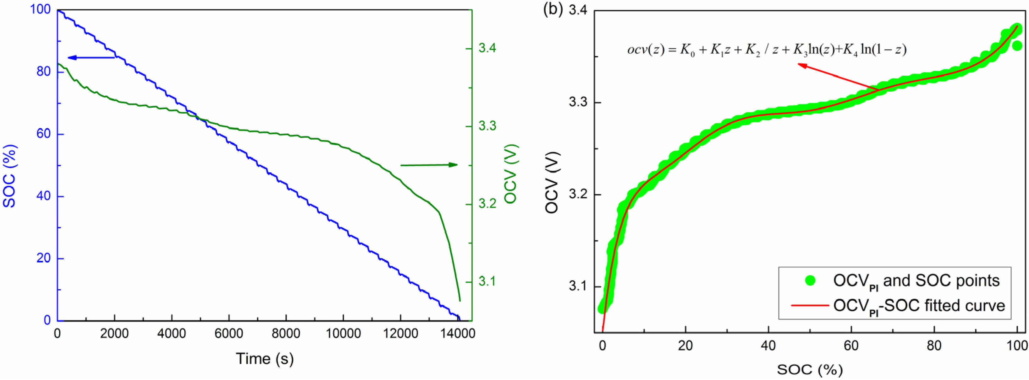
Nevertheless, the preceding analyses are enlightening. If we establish the relationship between SOC and OCV using OCV_PI, then we may expect an accurate SOC estimation result. Considering this finding, we proposed a novel OCV–SOC relationship (i.e., OCV_PI–SOC), which could be developed by combining the online identification of OCV with the true SOC. In this study, true SOC was calculated via coulomb counting based on the load current profiles and coulomb efficiency map. In addition, the initial values of the parameters were set in small offsets based on the results in Section 5, which ensures an adequate short convergence process. For example, Figure 22a illustrates the online identification of the OCV and the true SOC curves in the DST test at 40 °C. Meanwhile, the scatter plot of OCV and SOC data points as dependent and independent variables, respectively, is depicted in Figure 22b. The points are substantially nonlinear, and a mathematical description for the electrochemical model in [11,19] fitted to the data captures the basic trend in the data.

$$ocv(z)=K_0+K_{1}z+K_2/z+K_3\ln (z)+K_{4}ln(1-z)$$

(18)

where $z$ is the SOC. $K_i$ $(i=0,1,\dots ,4)$ are the four polynomial coefficients that must fit the OCV–SOC curve. The fitted curve is shown in Figure 22b.

We have discussed how to develop OCV_PI–SOC only at one specific temperature. Considering the temperature dependence of OCV_PI–SOC curves, the parameters of the OCV function in Equation (18) are represented by a continuous polynomial of temperature (three order), as follows:

$$K_i=A_{i1}+A_{i2}\times T+A_{i3}\times T^2+A_{i4}\times T^3(i=0,1,\dots ,4)$$

(19)

where $T$ is the ambient temperature ranging from 0 °C–40 °C. $A_{i1}~A_{i4}$ $(i=0,1,\dots ,4)$ are the four polynomial coefficients that must fit the OCV_PI–SOC–T relationship map, which is plotted in Figure 23.

Figure 22. Establishing OCV_PI-SOC relationship in the DST test at 40 °C: (a) online identification of the OCV and the true SOC and (b) the scatter plot and fitted curve of OCV_PI and the true SOC.

Figure 22. Establishing OCV_PI-SOC relationship in the DST test at 40 °C: (a) online identification of the OCV and the true SOC and (b) the scatter plot and fitted curve of OCV_PI and the true SOC.

Figure 23. OCV_PI–SOC–T relationship map.

Figure 23. OCV_PI–SOC–T relationship map.

For computations involving SOC, the final relationship map of OCV_PI–SOC–T was digitized at 201 × 41 points (SOC interval 0.5%, temperature interval 1 °C) and stored in a table. Linear interpolation was used to search for the values in the table.

6.2. Verifying SOC Estimation

To verify the generality of the OCV_PI–SOC–T relationship map built by the DST profile, a FUDS test with a sophisticated dynamic current profile was performed. In addition, the OCV_VR–SOC–T and OCV_CT–SOC–T relationship maps were used to compare the estimations and validate the effectiveness of the proposed OCV–SOC relationship. Furthermore, the verification experiment for SOC estimation was conducted from 0 °C–40 °C at an interval of 10 °C. This test aimed to evaluate the adaptability of the estimation method under different temperatures.

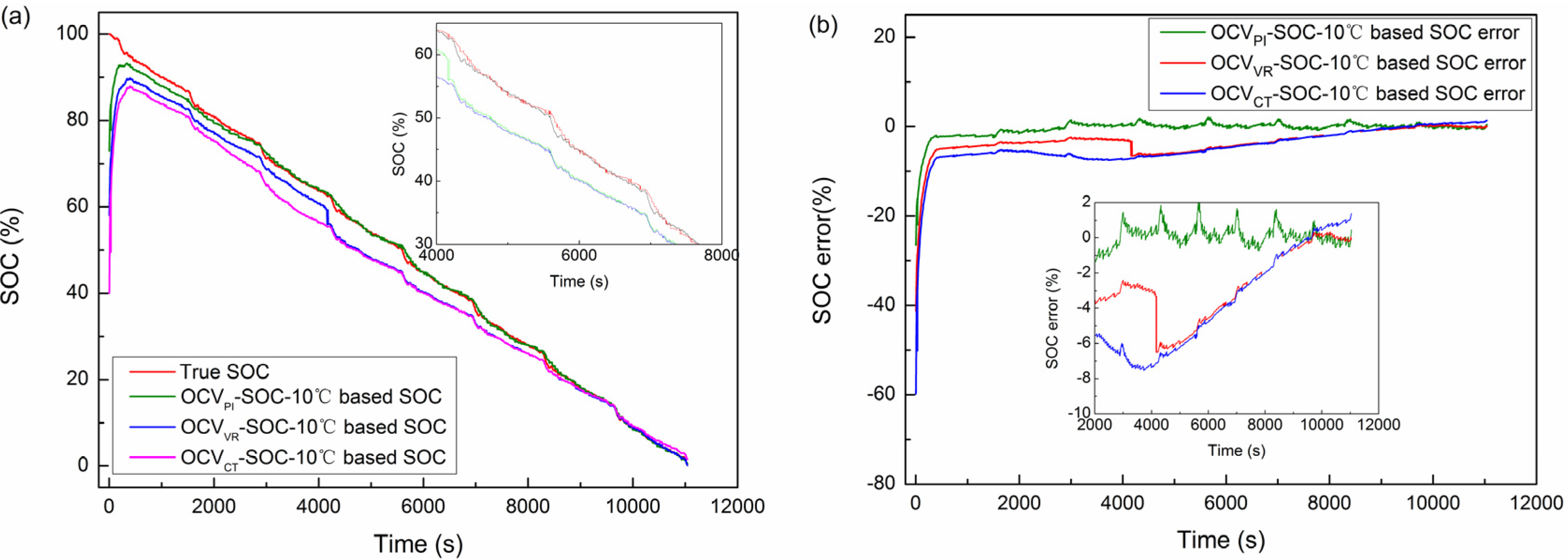
Figure 24 shows the estimation results for SOCs and SOC errors in the DST test at 40 °C. Figure 24a shows the estimated SOCs for the three OCV–SOC–40 °C relationship maps (i.e., OCV_PI–SOC–40 °C, OCV_VR–SOC–40 °C, and OCV_CT–SOC–40 °C). The SOC estimation errors between the estimations and the true SOC are given in Figure 24b. As shown in Figure 24, the estimated SOC based on the OCV_PI–SOC–40 °C relationship map traces the trajectory of the true SOC accurately. By using the OCV_VR–SOC–40 °C and OCV_CT–SOC–40 °C relationship maps, a large negative deviation from the true SOC was observed. This result was attributed to two reasons. First, the effects of concentration polarization and hysteresis were not included in the two relationship maps, which resulted in OCV_VR and OCV_CT that are larger than OCV_PI in the same SOC. Second, LiFePO₄ batteries exhibit a flat OCV curve in large SOC ranges and a long charge/discharge voltage plateau. Thus, even a small deviation from OCV inference causes a large fluctuation in the estimated SOC.

Figure 24. Estimated comparison using the three different OCV–SOC–T relationship maps in the FUDS test at 40 °C: (a) SOC and (b) SOC error.

Figure 24. Estimated comparison using the three different OCV–SOC–T relationship maps in the FUDS test at 40 °C: (a) SOC and (b) SOC error.

Figure 25, Figure 26, Figure 27 and Figure 28 show the comparative profiles of SOCs and SOC errors using the three different OCV–SOC–T relationship maps in the FUDS test from 30 °C–0 °C. The statistical analysis of SOC errors is shown in Table 2. When the OCV_PI–SOC–T relationship map was selected to estimate SOC overall operating temperatures, the maximum error and the root mean square (RMS) error were less than 4.02% and 2.24%, respectively. Moreover, the errors of the estimated SOC increase as temperature decreases because the accuracy of voltage estimation at low temperature is slightly less than that at high temperature, as mentioned in Section 5. The large voltage estimation error at low temperature is partially embedded into the result of OCV identification at low temperature. By using the OCV_VR–SOC–T and OCV_CT–SOC–T relationship maps, the maximum and RMS errors were both larger than those based on the OCV_PI–SOC–T map at each temperature because of the large voltage of concentration polarization and hysteresis at low temperature.

Figure 25. Estimated comparison using the three different OCV–SOC–T relationship maps in the FUDS test at 30 °C: (a) SOC and (b) SOC error.

Figure 25. Estimated comparison using the three different OCV–SOC–T relationship maps in the FUDS test at 30 °C: (a) SOC and (b) SOC error.

Figure 26. Estimated comparison using the three different OCV–SOC–T relationship maps in the FUDS test at 20 °C: (a) SOC and (b) SOC error.

Figure 26. Estimated comparison using the three different OCV–SOC–T relationship maps in the FUDS test at 20 °C: (a) SOC and (b) SOC error.

Figure 27. Estimated comparison using the three different OCV–SOC–T relationship maps in the FUDS test at 10 °C: (a) SOC and (b) SOC error.

Figure 27. Estimated comparison using the three different OCV–SOC–T relationship maps in the FUDS test at 10 °C: (a) SOC and (b) SOC error.

Figure 28. Estimated comparison using the three different OCV–SOC–T relationship maps in the FUDS test at 0 °C: (a) SOC and (b) SOC error.

Figure 28. Estimated comparison using the three different OCV–SOC–T relationship maps in the FUDS test at 0 °C: (a) SOC and (b) SOC error.

Table 2. List of statistics of SOC estimation errors with different OCV–SOC–T relationship maps.

Temperature (°C)	Maximum Error (%)			RMS Error (%)
	OCVPI-SOC-T	OCVVR-SOC-T	OCVCT-SOC-T	OCVPI-SOC-T	OCVVR-SOC-T	OCVCT-SOC-T
40 °C	1.3403	4.9674	5.4576	0.6408	2.6458	3.1622
30 °C	1.4709	5.2423	6.0818	0.6823	2.3449	3.6874
20 °C	1.6288	5.9237	6.6250	0.8019	2.6858	4.0969
10 °C	2.4455	6.5152	7.5307	1.2857	3.3993	4.6280
0 °C	4.0177	8.8833	9.4587	2.2417	5.7586	5.5920

Table 2. List of statistics of SOC estimation errors with different OCV–SOC–T relationship maps.

Temperature (°C)	Maximum Error (%)			RMS Error (%)
	OCVPI-SOC-T	OCVVR-SOC-T	OCVCT-SOC-T	OCVPI-SOC-T	OCVVR-SOC-T	OCVCT-SOC-T
40 °C	1.3403	4.9674	5.4576	0.6408	2.6458	3.1622
30 °C	1.4709	5.2423	6.0818	0.6823	2.3449	3.6874
20 °C	1.6288	5.9237	6.6250	0.8019	2.6858	4.0969
10 °C	2.4455	6.5152	7.5307	1.2857	3.3993	4.6280
0 °C	4.0177	8.8833	9.4587	2.2417	5.7586	5.5920

7. Conclusions

An online estimation method for model parameters and SOC is proposed in this study for applications in EVs under various temperatures. To address model parameter fluctuations under different temperatures, the AJEKF algorithm is developed by exploiting KF and employed based on an RC-circuit model for the online estimation of model parameters. The simulations and experiments verify the accurate regression capability and good performance of the proposed algorithm in predicting dynamic voltage behavior.

To achieve accurate SOC estimates, a novel OCV_PI–SOC–temperature relationship map is established after the complete discussion of two conventional OCV determination methods. A validation experiment is performed based on consecutive loading profiles to assess SOC estimation performance. A comparison is made between the novel and the two conventional relationship maps. The results indicate that our method is effective and adaptable when a battery operates at different ambient temperatures.

The research reported in this paper is primarily aimed for a single battery. Future work will focus on battery pack SOC estimation to consider inconsistencies among cells.

References

1. Yao, J.; Wu, F.; Qiu, X.; Li, N.; Su, Y. Effect of CeO2-coating on the electrochemical performances of LiFePO4/C cathode material. Electrochim. Acta 2011, 56, 5587–5592. [Google Scholar]
2. Xing, Y.; Ma, E.W.M.; Tsui, K.L.; Pecht, M. Battery management systems in electric and hybrid vehicles. Energies 2011, 4, 1840–1857. [Google Scholar] [CrossRef]
3. Andrea, D. Battery Management Systems for Large Lithium Ion Battery Packs, 1st ed.; Artech House: London, UK, 2010; pp. 22–110. [Google Scholar]
4. Chung, S.Y.; Bloking, J.T.; Chiang, Y.M. Electronically conductive phospho-olivines as lithium storage electrodes. Nat. Mater. 2002, 1, 123–128. [Google Scholar] [CrossRef] [PubMed]
5. Christopher, M.; Burba, R.F. Local structure in the Li-ion battery cathode material Lix(MnyFe1-y)PO4 for 0 < x ≤ 1 and y = 0.0, 0.5 and 1.0. J. Power Sour. 2007, 172, 870–876. [Google Scholar] [CrossRef]
6. Andersson, A.S.; Thomas, J.O. The source of first-cycle capacity loss in LiFePO4. J. Power Sour. 2001, 97–98, 498–502. [Google Scholar] [CrossRef]
7. Kang, L.; Zhao, X.; Ma, J. A new neural network model for the state-of-charge estimation in the battery degradation process. Appl. Energy 2014, 121, 20–27. [Google Scholar] [CrossRef]
8. Feng, R.; Zhao, S.; Lu, X. On-line estimation of dynamic state-of-charge for lead acid battery based on fuzzy logic. In Proceedings of the IEEE 2nd International Conference on Measurement, Information and Control (ICMIC’13), Harbin, China, 16–18 August 2013; pp. 702–707. [CrossRef]
9. Juan, C.A.A.; Paulino, J.G.N.; Cecilio, B.V.; Jose, A.V.V. Support vector machines used to estimate the battery state of charge. IEEE Trans. Power Electron. 2013, 28, 5919–5926. [Google Scholar] [CrossRef]
10. Plett, G.L. Extended Kalman filtering for battery management systems of LiPB-based HEV battery packs: Part 1. Background. J. Power Sources 2004, 134, 252–261. [Google Scholar] [CrossRef]
11. Plett, G.L. Extended Kalman filtering for battery management systems of LiPB-based HEV battery packs: Part 2. Modeling and identification. J. Power Sources 2004, 134, 262–276. [Google Scholar] [CrossRef]
12. Plett, G.L. Extended Kalman filtering for battery management systems of LiPB-based HEV battery packs: Part 3. State and parameter estimation. J. Power Sources 2004, 134, 277–292. [Google Scholar] [CrossRef]
13. Plett, G.L. Sigma-point Kalman filtering for battery management systems of LiPB-based HEV battery packs: Part 1. Introduction and state estimation. J. Power Sources 2006, 161, 1356–1368. [Google Scholar] [CrossRef]
14. Plett, G.L. Sigma-point Kalman filtering for battery management systems of LiPB-based HEV battery packs: Part 2. Simultaneous state and parameter estimation. J. Power Sources 2006, 161, 1369–1384. [Google Scholar] [CrossRef]
15. Sun, F.; Hu, X.; Zou, Y.; Li, S. Adaptive unscented Kalman filtering for state of charge estimation of a lithium-ion battery for electric vehicles. Energies 2011, 36, 3531–3540. [Google Scholar] [CrossRef]
16. He, W.; Williard, N.; Chen, C.; Pecht, M. State of charge estimation for electric vehicle batteries using unscented Kalman filtering. Microelectron. Reliabil. 2013, 53, 840–847. [Google Scholar] [CrossRef]
17. Schwunk, S.; Armbruster, N.; Straub, S.; Kehl, J.; Vetter, M. Particle filter for state of charge and state of health estimation for lithium–iron phosphate batteries. J. Power Sources 2013, 239, 705–710. [Google Scholar] [CrossRef]
18. He, Y.; Liu, X.; Zhang, C.; Chen, Z. A new model for State-of-Charge (SOC) estimation for high-power Li-ion batteries. Appl. Energy 2013, 101, 808–814. [Google Scholar] [CrossRef]
19. Xiong, R.; Sun, F.; Gong, X.; Gao, C. A data-driven based adaptive state of charge estimator of lithium-ion polymer battery uesd in electric vehicles. Appl. Energy 2013, 113, 1421–1433. [Google Scholar] [CrossRef]
20. Xing, Y.; He, W.; Pecht, M.; Tsui, K. State of charge estimation of lithium-ion batteries using the open-circuit voltage at various ambient temperatures. Appl. Energy 2014, 113, 106–115. [Google Scholar] [CrossRef]
21. He, H.; Xiong, R.; Gao, H. Online estimation of model parameters and state-of-charge of LiFePO4 batteries in electric vehicles. Appl. Energy 2014, 89, 413–420. [Google Scholar] [CrossRef]
22. Xiong, R.; He, H.; Sun, H.; Zhao, K. Evaluation on state of charge estimation of batteries with adaptive extended Kalman filiter by experiment approach. IEEE Trans. Veh. Technol. 2013, 62, 108–117. [Google Scholar] [CrossRef]
23. Pei, L.; Zhu, C.; Wang, T.; Lu, R.; Chan, C. Online peak power prediction based on a parameter and state estimator for lithium-ion batteries in electric vehicles. Energy 2014, 66, 766–778. [Google Scholar] [CrossRef]
24. He, H.; Xiong, R.; Zhang, X.; Sun, F.; Fan, J. State-of-charge estimation of the lithium-ion battery using an adaptive extended Kalman filter based on an improved thevenin Model. IEEE Trans. Veh. Technol. 2011, 60, 1461–1469. [Google Scholar] [CrossRef]
25. Seongjun, L.; Jonghoon, K.; Jaemoon, L.; Cho, B. State-of-charge and capacity estimation of lithium-ion battery using a new open-circuit voltage versus state-of-charge. J. Power Sources 2008, 185, 1367–1373. [Google Scholar] [CrossRef]
26. Hu, X.; Li, S.; Peng, H. A comparative study of equivalent circuit models for Li-ion batteries. J. Power Sources 2011, 198, 359–367. [Google Scholar] [CrossRef]
27. Wan, E.; Nelson, A. Dual extended Kalman filter methods. In Kalman Filtering and Neural Networks; John Wiley & Sons, Inc.: New York, NY, USA, 2002; pp. 123–173. [Google Scholar]
28. Mohamed, A.; Schwarz, K. Adaptive Kalman filtering for INS/GPS. J. Geodesy 1999, 73, 193–203. [Google Scholar] [CrossRef]
29. Feng, F.; Lu, R.; Zhu, C. A combined state of charge estimation method for lithium-ion batteries used in a wide ambient temperature range. Energies 2014, 7, 3004–3032. [Google Scholar] [CrossRef]
30. USABC and DOE National Laboratories personnel. USABC Battery Test Procedures Manual. 1996. Available online: http://avt.inl.gov/battery/pdf/usabc_manual_rev2.pdf (accessed on 10 January 1996).
31. He, H.; Zhang, X.; Xiong, R.; Xu, Y.; Gao, H. Online model-based estimation of state-of-charge and open-circuit voltage of lithium-ion batteries in electric vehicles. Energy 2012, 39, 310–318. [Google Scholar] [CrossRef]
32. Dai, H.; Wei, X.; Sun, Z.; Wang, J.; Gu, W. Online cell SOC estiamtion of Li-ion battery packs using a dual time-scale Kalman filtering for EV applications. Appl. Energy 2012, 95, 227–237. [Google Scholar] [CrossRef]