
Toward Isolation of Salient Features in Stable Boundary Layer Wind Fields that Influence Loads on Wind Turbines


Abstract
: Neutral boundary layer (NBL) flow fields, commonly used in turbine load studies and design, are generated using spectral procedures in stochastic simulation. For large utility-scale turbines, stable boundary layer (SBL) flow fields are of great interest because they are often accompanied by enhanced wind shear, wind veer, and even low-level jets (LLJs). The generation of SBL flow fields, in contrast to simpler stochastic simulation for NBL, requires computational fluid dynamics (CFD) procedures to capture the physics and noted characteristics—such as shear and veer—that are distinct from those seen in NBL flows. At present, large-eddy simulation (LES) is the most efficient CFD procedure for SBL flow field generation and related wind turbine loads studies. Design standards, such as from the International Electrotechnical Commission (IEC), provide guidance albeit with simplifying assumptions (one such deals with assuming constant variance of turbulence over the rotor) and recommend standard target turbulence power spectra and coherence functions to allow NBL flow field simulation. In contrast, a systematic SBL flow field simulation procedure has not been offered for design or for site assessment. It is instructive to compare LES-generated SBL flow fields with stochastic NBL flow fields and associated loads which we evaluate for a 5-MW turbine; in doing so, we seek to isolate distinguishing characteristics of wind shear, wind veer, and turbulence variation over the rotor plane in the alternative flow fields and in the turbine loads. Because of known differences in NBL-stochastic and SBL-LES wind fields but an industry preference for simpler stochastic simulation in design practice, this study investigates if one can reproduce stable atmospheric conditions using stochastic approaches with appropriate corrections for shear, veer, turbulence, etc. We find that such simple tuning cannot consistently match turbine target SBL load statistics, even though this is possible in some cases. As such, when there is a need to consider different stability regimes encountered by a wind turbine, easy solutions do not exist and large-eddy simulation at least for the stable boundary layer is needed.1. Introduction
In recent years, wind energy has witnessed faster growth worldwide than almost all other renewables, with the exception of solar energy. Aggressive renewable portfolio standards have sought to increase the percentage of renewable sources in the energy portfolios of many states in the United States; this, along with production tax credits, has led to a boom in wind-generated electricity production. While this is encouraging news, some challenges have become evident. First, models used in the design process—as defined, say, in the International Electrotechnical Commission (IEC) design standards—for simulating turbulence do not cover the range of atmospheric conditions associated with critical events (e.g., strong shear and veer across a turbine rotor). Second, turbines in service are aging and failures especially due to fatigue (composite materials used for blades are especially vulnerable) demand attention. Finally, an experience base on turbine usage has been accumulated and gaps have been identified: refinements in design philosophy and practice are needed that are informed by improved capabilities in atmospheric boundary layer (ABL) modeling (e.g., by the use of large-eddy simulation (LES)) and wind turbine aeroelastic response simulations. At present, the IEC guidelines explicitly address conditions associated only with the neutral boundary layer (NBL)—i.e., they ignore buoyancy effects in the definition of design load cases. In the present work and in ongoing studies [1–4], the authors are seeking to extend the design paradigm to allow a reliability-based assessment of wind turbines against fatigue and extreme limit states that includes evaluation of turbine loads for suites of inflow turbulence flow fields that have the spatial structure and characteristics that reflect a wide range of atmospheric stability conditions.
Today’s utility-scale wind turbines have blade tips that, at their highest points, extend up to 150 m above ground level (AGL) and higher; new rotors are expected to sweep heights above 200 m. As turbine rotors and hub heights have gotten larger, concerns have arisen about the need to model realistic atmospheric flows that can cause complex forces on the rotors such as significant asymmetrical loadings due to high wind speed and directional shear. Such conditions are commonly observed in the night-time stable boundary layer (SBL). Existing design standards such as IEC 61400-1 [5], which specify inflow conditions in turbine design load cases to be checked, do not exhaustively consider all such complex loadings. In part due to the rapid evolution of machines to increasingly larger sizes—older machines were smaller and not as susceptible to such spatially complex and critical flow fields that today’s larger turbines experience—these design standards have been slow to adapt to needed changes and a revisiting of some of the design load case criteria for fatigue and ultimate limit states.
This study seeks to understand SBL wind fields. We use LES to simulate such fields. Despite the widely varying and complex flow field characteristics encountered in the atmospheric boundary layer, the IEC-approved approach only prescribes simulation of NBL wind fields and ignores directional shear (i.e., veer) and turbulence energy variation with elevation. Although such IEC-approved NBL simulation is physically unrealistic, in the present study, we use this both as a benchmark consistent with industry practice and to highlight differences and enhancements that result from the use of LES for the SBL. For ease of presentation, we will refer to this benchmark as IEC-NBL or merely as NBL in the following. Wind shear, veer, and elevation-dependent turbulence variance particularly in the SBL (as distinct from the same in the NBL) have been recognized as having a significant influence on power generated as well as on loads experienced by utility-scale wind turbines with large rotor-swept areas [6–8]. Physics-based large-eddy simulation can be used to describe various realistic flow fields including those for the SBL [1,2,4,9]; on the other hand, stochastic simulation [10] is the accepted method of choice for the generation of IEC-NBL flow fields and its use, with spectral methods, is well documented in design standards and guidelines.
Our goal in this study is to compare LES-generated SBL flow fields with stochastic NBL flow fields and associated loads which we evaluate for a 5-MW turbine; in doing so, we seek to isolate distinguishing characteristics of wind shear, wind veer, and turbulence variation over the rotor plane in the alternative flow fields and in the turbine loads. Because of known differences in NBL-stochastic and SBL-LES wind fields but an industry preference for simpler stochastic simulation in design practice, this study investigates if one can reproduce stable atmospheric conditions using stochastic approaches with appropriate corrections for shear, veer, turbulence, etc. a question that this study seeks to address is this: Can a stochastically simulated IEC-NBL wind field with missing flow features evident in physics-based SBL fields (and only possible to generate using LES) be modified so as to capture those missing features? Incremental adjustments on wind shear, veer, and turbulence variation are attempted and loads for the baseline IEC-NBL (without adjustments), for the target LES-SBL, and for a stepwise modified baseline are compared.
1.1. Procedure for Analysis
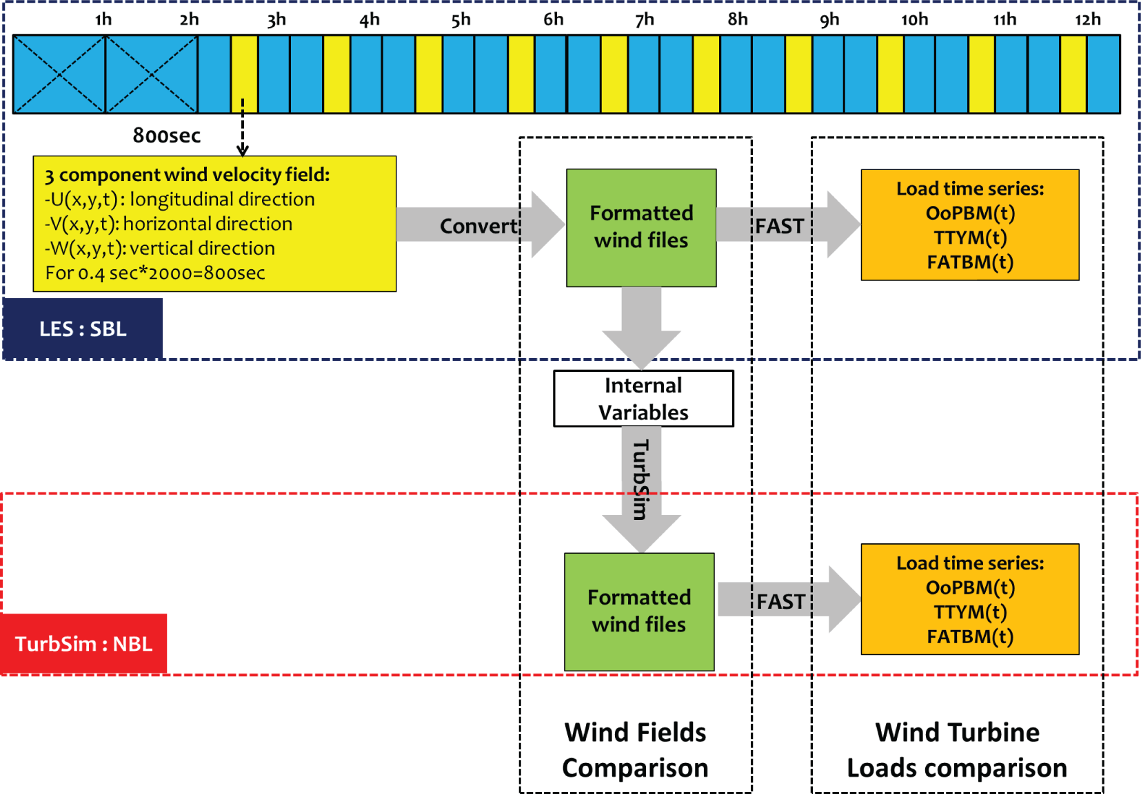
Figure 1 shows a schematic flow chart describing the comparison study that we undertake with SBL and NBL flow fields. For the LES flow fields, an in-house large-eddy simulation code (called MATLES) is utilized for turbulent inflow generations. Salient features of the MATLES code are described in the work of Basu and Porté-Agel [11]. These LES-SBL flow fields provide 12 h of output. For loads computed using the open-source software, FAST [12], the inflow fields are provided as 800-second time series of three wind velocity components generated every hour, beginning from the third until the twelfth hour, over the rotor plane of the selected 5-MW turbine model [13]. From each turbine response simulation, we evaluate loads—three different loads are considered here; they include the blade root out-of-plane bending moment (OoPBM), the tower-top yawing moment (TTYM), and the base fore-aft tower bending moment (FATBM). Extreme and fatigue loads are evaluated. When needed, baseline stochastic IEC-NBL flow fields are generated using TurbSim [10] by matching the hub-height wind speed and wind shear that result from the associated LES-SBL runs to which comparison is made. The NBL flow fields are also input to the turbine model using FAST and loads are compared. a total of 2200 SBL runs provide 10-min load time series (the initial 200 s out of the available 800 s from each FAST simulation are discarded to avoid the influence of dynamic vibratory response transients). These 2200 SBL flow field time series arise from 44 separate environmental conditions (listed in Table 1) that we refer to as “external” variables. In our NBL versus SBL flow and load comparisons, we will sometimes seek to separate out flow regimes into subsets.
1.2. LES-SBL Computational Framework and External Variables
In LES studies involving the atmospheric boundary layer, it is generally the case that highly idealized or observed soundings or 1-D vertical profiles of velocity and other variables (such as potential temperature) are used together with small-scale random perturbations (noise) to generate initialization fields. Using the governing filtered Navier-Stokes equations and prognostic equations for other scalar variables (such as potential temperature), these fields are allowed to evolve in time under specified constraints from large-scale forcing effects (such as from the geostrophic wind) and subject to specified boundary conditions (such as, say, prescribed surface temperature). Depending on the characteristics of the boundary layer to be simulated, an initial transient period is needed before realistic turbulence can be generated (i.e., before development of the inertial-range spectra of turbulence).
In this study, large-scale atmospheric and surface conditions used as inputs or initial conditions for the LES computations are termed “external” variables. The following seven external variables are varied as LES inputs:
G, Geostrophic wind speed
C, Surface cooling rate
z0, Aerodynamic roughness length
Hi, Initial height of boundary layer
N, Inversion strength
f, Coriolis frequency
DG, Geostrophic departure
A detailed description of the flow fields simulated using LES is reported by Park et al. [4]. Here, we note that for the initial profiles, the longitudinal velocity (units: m/s), U(z), is such that U(z) = G − DG for z0 < z < Hi and U(z) = G for z ≥ Hi; the lateral velocity, V (z), and the vertical velocity, W (z), are both zero for z > z0; and potential temperature (units: K), θ(z), is such that θ(z) = 300 for z0 < z < Hi and θ(z) = 300 + N(z − Hi) for z ≥ Hi. These fields are evolved under the constraints of specified large-scale forcing (geostrophic wind) and surface boundary conditions (prescribed temperature). Random Gaussian noise with a standard deviation of 0.1 m/s and 0.1 K are added to the lowest 100 m of the vertical velocity and potential temperature fields, respectively. In the present study, it takes about an hour of simulation for each case studied to generate realistic turbulence.
Time-height independent geostrophic wind speed (representing a barotropic SBL) serves as the forcing term for the LES runs. In a few cases, DG is assumed to be positive below Hi to represent a decrease in wind speed from the geostrophic value due to turbulent mixing; above Hi, DG is assumed to be zero. In several earlier studies, sensible heat flux has been used as a lower boundary condition [14–16]. Some shortcomings resulting from the use of such sensible heat flux-based lower boundary conditions have been discussed by Basu et al. [17]. It was shown that if surface sensible heat flux is prescribed as a boundary condition, only near-neutral to weakly stable regimes can be represented; for moderately stable to very stable regimes, surface temperature prescription is needed. For these reasons, we use surface temperature as a lower boundary condition. It is for this reason that the surface cooling rate (C; unit: K/h) is kept at a constant value in the LES runs in this study. Additional details on surface temperature-based or near-surface air temperature-based lower boundary condition can be found in several published studies [11,17–20]. We note that all our simulations include the Coriolis term representative of mid-latitude northern hemisphere (approximately 30°–60°) scenarios. Realistic wind veer as well as low-level jet (LLJ) formation (due to inertial oscillation) are feasible only if this Coriolis term is included.
Forty-four different combination of the selected external variables—i.e., G, C, zo, Hi, N, f, and DG—are considered in this study (see Table 1). In particular, note that Run No. 12 (denoted as CONTROL) represents a single special case; we use this control case extensively in contrasting the LES-SBL and the stochastic NBL wind velocity fields.
The spatial domain for all the LES-SBL runs is 800 m × 800 m × 790 m corresponding to Lx × Ly × Lz. This domain is divided into an 80 × 80 × 80 grid (i.e., grid resolution of 10 m × 10 m × 10 m). The computational spatial domain and grid resolution are similar to those used in related studies [15,19,21,22]. A time step of 0.1 s is used for all the runs; each run is of 12 h duration, involving 432,000 time steps. Simulated velocity and potential temperature fields output every 4th time step (i.e., at an output frequency of 2.5 Hz) are generated on two-dimensional cross-sections (representing y − z planes taken at x = 400 m). As such, every LES-SBL run generates four fields, corresponding to three velocity components (i.e., longitudinal, lateral, and vertical) as well as the potential temperature; also, each output field has dimensions 80 × 80 × 108,000. The three velocity fields are collocated in space using interpolation and are merged into a single data file.
1.3. Internal Variables
Flow variables at turbine scale are referred to as “internal” variables in this study; these are in contrast to the large-scale external variables defining the atmospheric boundary layer. Traditionally, the hub-height longitudinal ten-minute mean wind speed, Uh, and turbulence standard deviation, σU, have been considered turbine-scale flow variables of interest, especially in turbine load calculations. We consider those two variables as well as a wind shear-related variable, namely, the power-law exponent, α, for wind speed shear. Note that all of these are inter-related and depend on the atmospheric stability regime; such stability-related variables have been the subject of other studies where their correlation to turbine loads has also been discussed [4,6–8].
It is convenient to normalize α and σU so as to have a zero mean and a unit standard deviation as follows:
zα < 0 ∩ zσ > 0: weak shear and strong turbulence
zα > 0 ∩ zσ > 0: strong shear and strong turbulence
zα < 0 ∩ zσ < 0: weak shear and weak turbulence
zα > 0 ∩ zσ < 0: strong shear and weak turbulence
This classification of flow field characteristics will be used in this study when we relate turbine-scale flow field characteristics to various wind turbine load statistics and we compared LES-SBL and stochastic NBL simulations.
2. Contrasting Characteristics of LES-SBL and Stochastic NBL Wind Fields
We discuss first differences in characteristics of simulated SBL and NBL wind fields. From each of the 2200 LES-generated SBL wind fields, the hub-height longitudinal mean wind speed, Uh, and standard deviation, σU, were determined; then, with these matching Uh and σU values as inputs, 2200 stochastic simulations were generated for NBL flow fields (assuming Kaimal turbulence power spectra, exponential coherence functions, constant turbulence variation over the rotor, and a power-law wind shear exponent, α, of 0.2).
2.1. Mean Wind Speed Vertical Profile
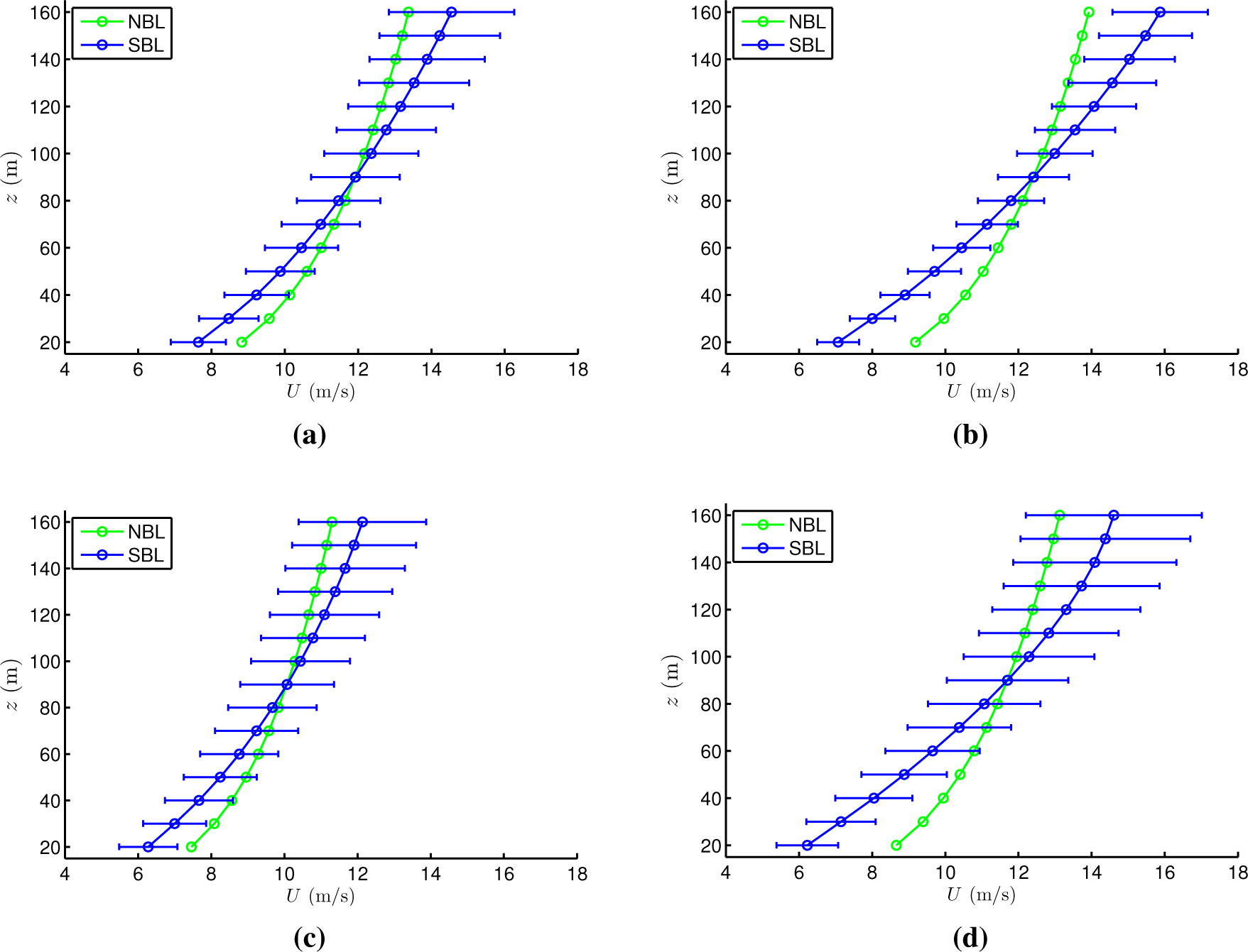
Figure 2 compares ensemble-averaged mean wind profiles for the SBL and NBL wind fields for elevations ranging from 20 m to 160 m above the ground, corresponding to the range of heights above ground of interest for the 5-MW turbine that is discussed in this study. In each plot, the green circles represent the ensemble-averaged mean wind speed at elevation, z, above ground for the NBL wind fields while the blue circles represent the same but for the SBL wind fields. The error bars indicate one standard deviation of the mean wind speed for the SBL wind fields. It can be seen that the SBL mean wind profiles deviate from those for the NBL case most noticeably in those LES runs (Figure 2b,d) where strong shear results from the imposed environmental conditions (due to the faster surface cooling rates). In the SBL case, the mean wind speed variation between the rotor top and bottom can be up to twice as great as that in the NBL case.
2.2. Mean Wind Direction Vertical Profile
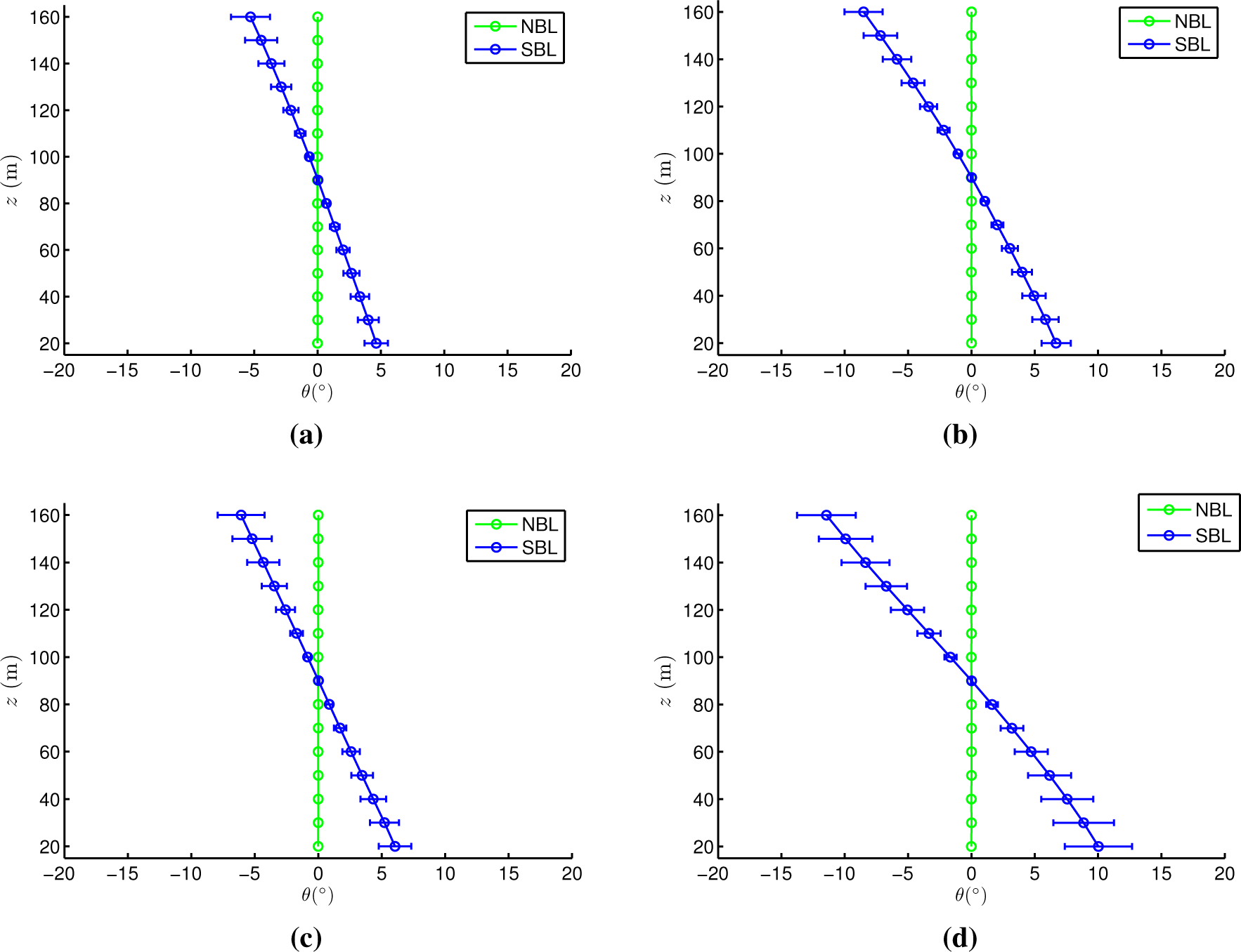
Figure 3 compares ensemble-averaged mean wind direction profiles for the SBL and NBL wind fields. As before, the green circles represent the ensemble-averaged mean wind direction at elevation, z, above ground for the NBL wind fields while the blue circles represent the same for the SBL wind fields. The error bars indicate one standard deviation of the mean wind direction for the SBL wind fields. We note that there is a systematic mean wind direction variation with elevation only in the SBL case; this wind veer is expected in the stable boundary layer. While the SBL mean wind direction variation is almost linear with elevation, there is no mean wind direction variation with height for the NBL. Note that the NBL flow fields were generated after the SBL runs were completed. For the sake of comparison, the LES-generated SBL flow fields were rotated so as to have a zero-mean lateral velocity component at hub height (90 m, for the selected 5-MW turbine); this is why both the SBL and NBL cases have a zero wind direction at hub height. In load studies that follow, nacelle yaw misalignment differences between the NBL and SBL cases are minimized as a resultant of this rotation imposed on the SBL flow field.
Comparing mean wind direction profiles between the left and right pairs of plots in Figure 3, the gradients in cases (b) and (d) are noticeably larger than those in (a) and (c). Comparing Figures 2 and 3, it is clear that strong wind shear is accompanied by strong wind veer. Comparing the mean wind direction profiles between the top and bottom pairs of plots in Figure 3, we note that the gradients in the stronger turbulence regimes, (a) and (b), are somewhat smaller than those for the cases with weaker turbulence ((c) and (d)).
2.3. Turbulence Standard Deviation Vertical Profile
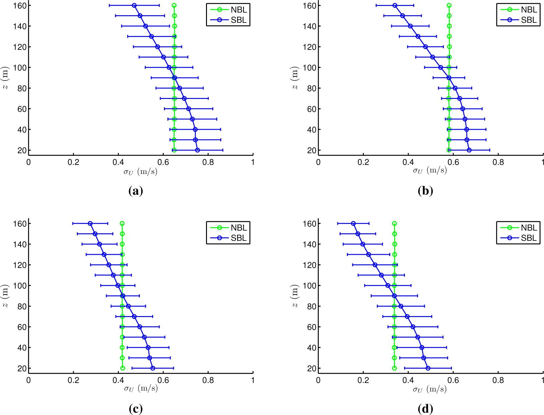
Figure 4 compares ensemble-averaged profiles of the standard deviation of the longitudinal wind velocity (σU) for the SBL and NBL wind fields. As before, the green circles apply to the NBL wind fields, while the blue circles apply to the SBL wind fields. The error bars indicate one standard deviation values of σU on the profiles for the SBL wind fields. Turbulence levels for the SBL case clearly decrease with elevation, whereas they are constant at all elevations for the NBL case (this is by intent in stochastic simulation per IEC guidelines). Larger turbulence levels at lower levels that decrease with height are more realistic due to surface friction effects that diminish with elevation above ground. Wind velocity standard deviation profiles in stronger turbulence regimes, i.e., cases (a) and (b), show varying gradients with height—below the rotor hub (90 m), the turbulence increases at a lower rate than its rate of decrease above the rotor hub. Note that the NBL flow fields were generated so as to have matching longitudinal mean wind speed and standard deviation at hub height as that from the SBL flow fields.
3. Isolation of SBL Flow Field Features in Simulated NBL Fields
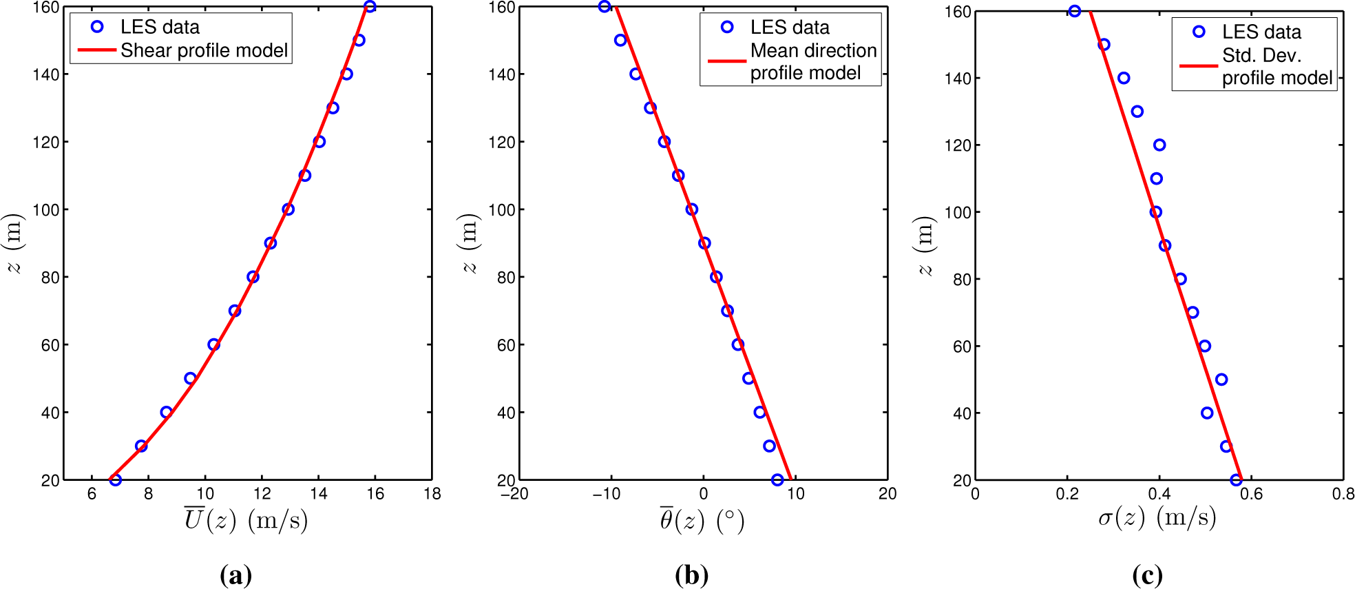
Based on the preceding observations regarding vertical profiles of the mean wind speed, mean wind direction, and turbulence standard deviation, which we denote, respectively, as , , and σ(z) (such that at hub height, zh, we have , , and σ(z) = σU), we can make linear least-squares fits of SBL-generated profiles using three variables, , Ŝθ, and Ŝσ. Thus, we can express , , and σ(z) as follows:
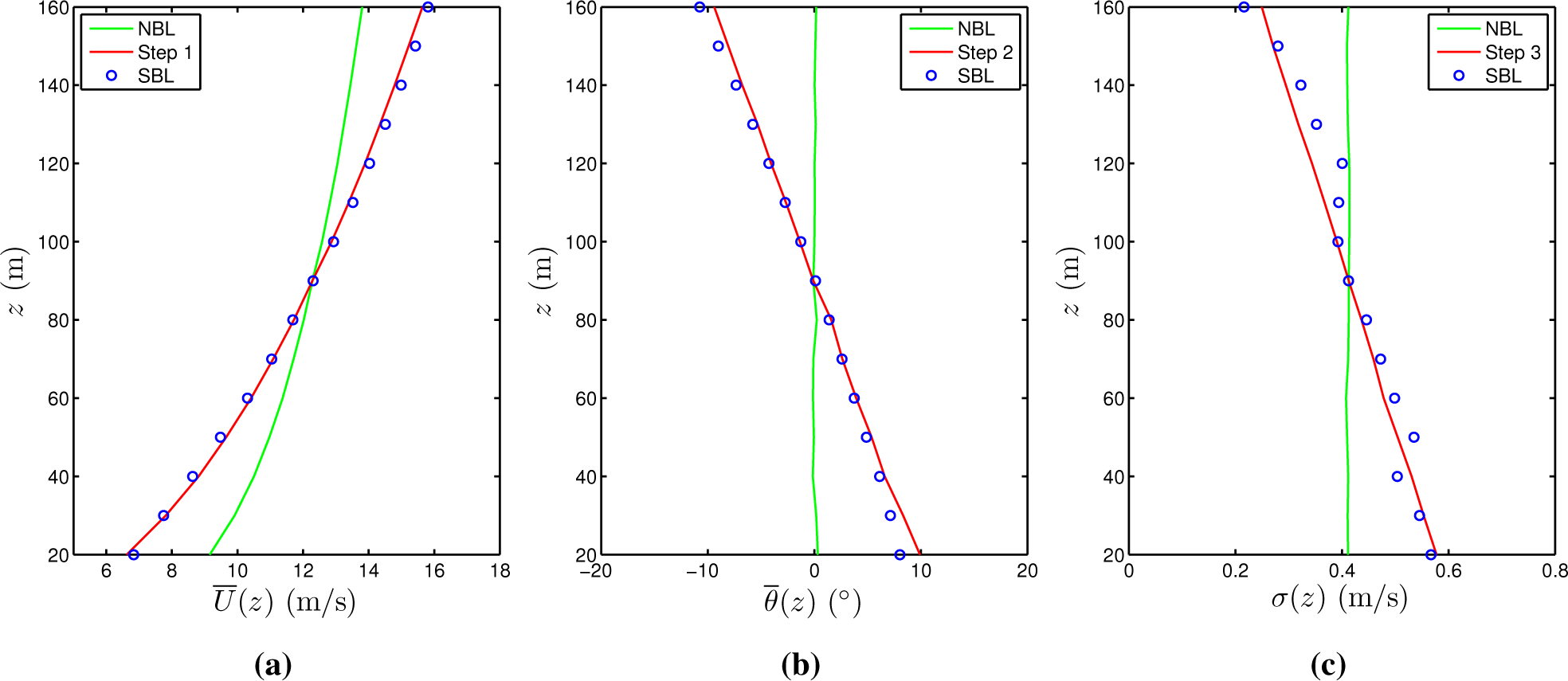
For a single LES run (taken from the last hour of a 12-hour simulation for the control case in Table 1), profiles based on fits using Equations (3)–(5) are shown along with the data in Figure 5. The three estimated parameters, , Ŝθ, and Ŝσ, serve to describe distinct SBL-associated wind field characteristics. From each of the 2200 LES runs, such parameters are estimated. The NBL flow fields previously discussed in Section 2 are now modified by adjusting their mean wind speed, mean wind direction, and turbulence standard deviation vertical profiles, one at a time to render them more “similar” to each associated SBL flow. By studying wind turbine loads from the SBL flow fields with those from such incrementally adjusted NBL flow fields, we seek to identify those flow characteristics that influence turbine loads.
To clarify, in the following, we are also interested in evaluating whether or not it is possible to achieve similar turbine load statistics for stochastically simulated NBL flow fields with adjustments to match corresponding SBL flow fields generated using LES. We note too that LES-SBL flow fields show patterns of combinations of turbine-scale internal variables that are inter-dependent (correlated) and it may not be possible to create in general the appropriate adjustments to vertical profiles for the internal variables in stochastic NBL flows as we have done here; nevertheless, we discuss next how loads from such “matched” NBL flows compare with those from SBL flows.
3.1. Modification of NBL Wind Fields With Adjustments for Mean Wind Speed, Mean Wind Direction, and Turbulence Standard Deviation
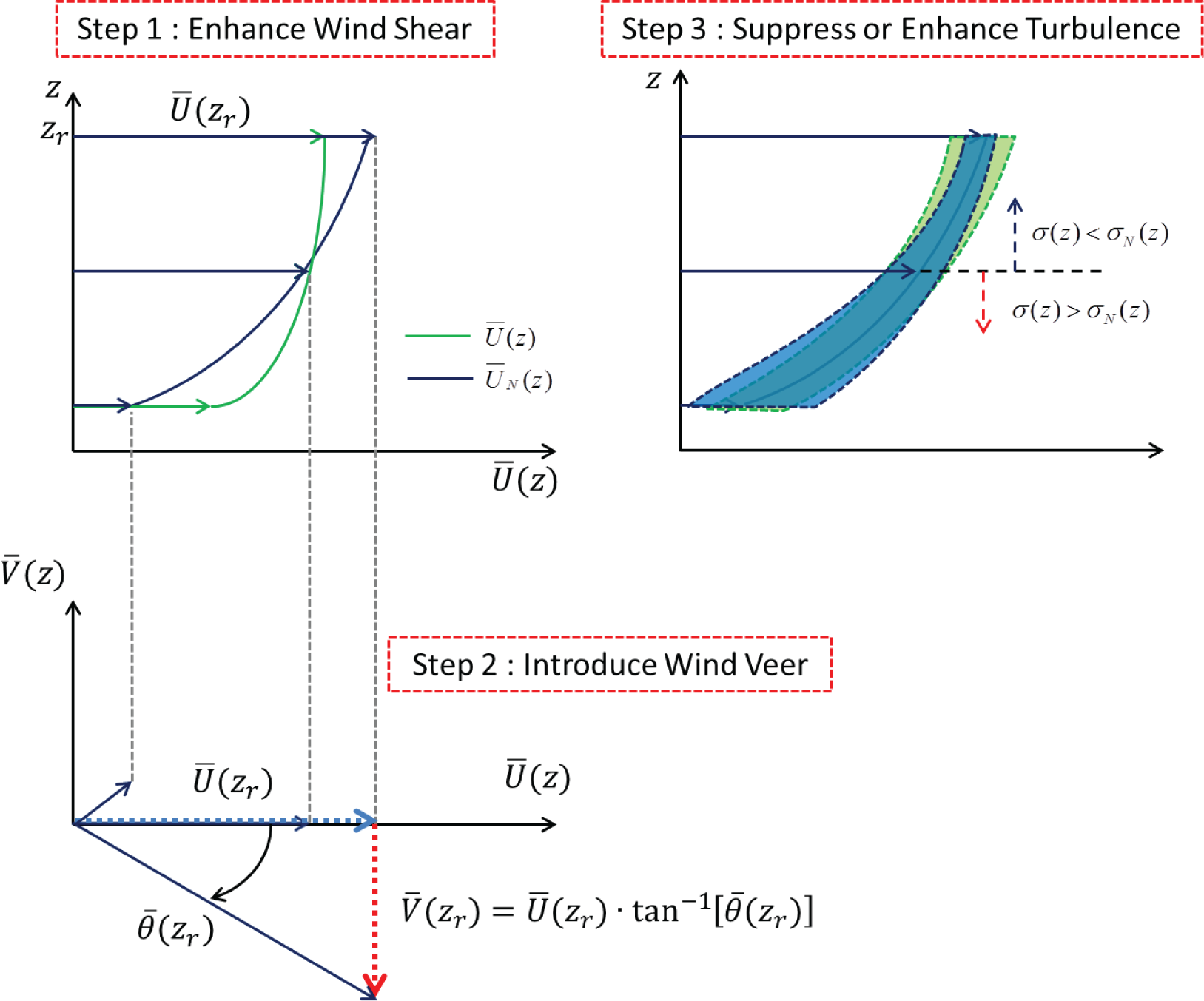
Figure 6 conceptually illustrates the procedure for adjusting NBL flow fields by successively enhancing wind shear (Step 1) using ; introducing wind veer (Step 2) using Ŝθ (note that this step effectively introduces a non-zero lateral wind velocity component, ); and suppressing or enhancing turbulence (Step 3) using Ŝσ (possibly at different slopes above and below the turbine hub height).
3.2. Illustration of Steps in Profile Correction
The single LES case presented in Figure 5 is considered to discuss the fitted parameters, , Ŝθ, and Ŝσ, first. These estimated parameters are summarized in Table 2. The three steps incrementally add one, then two, and finally three adjustments to the NBL flow field to match the target SBL flow field by use of the parameters in Table 2. In each step, the modifications made for profiles of mean wind speed, mean wind direction, and turbulence standard deviation are based on the estimated parameters; the red lines in Figure 7a–c show modified NBL profiles that closely match those based on the SBL data indicated by the blue circles. The green lines show the original unmodified NBL vertical profiles.
In the following, we now use the LES-SBL wind fields to compute loads. We also use stochastic-NBL wind fields with matching hub-height Uh and uniform σU profiles first and then follow this with step-wise adjustments of the NBL wind fields that are sequentially made to resemble the SBL wind fields. We compute loads for wind fields for the SBL, baseline stochastic NBL, Step 1 field (with shear adjustment), Step 2 (with veer adjustment added to Step 1), and Step 3 (with turbulence variation with height adjustment added to Step 2). The degree to which the step-wise adjustments to the baseline stochastic NBL wind field yields loads that match those for the LES-SBL wind field is a possible indicator of success in capturing important stable boundary layer characteristics stochastically.
3.3. Comparison of Wind Turbine Loads
For three loads—blade root out-of-plane bending moment (OoPBM), tower-top yawing moment (TTYM), and base fore-aft tower bending moment (FATBM)—we compare time series, power spectrum density functions, and stress range histograms for the SBL wind fields and for the NBL wind field, unmodified as well as with incremental modifications in three steps. This is done for the single LES run for which needed adjustments are indicated in Table 2.
3.3.1. Blade-Root Out-of-Plane Bending Moment
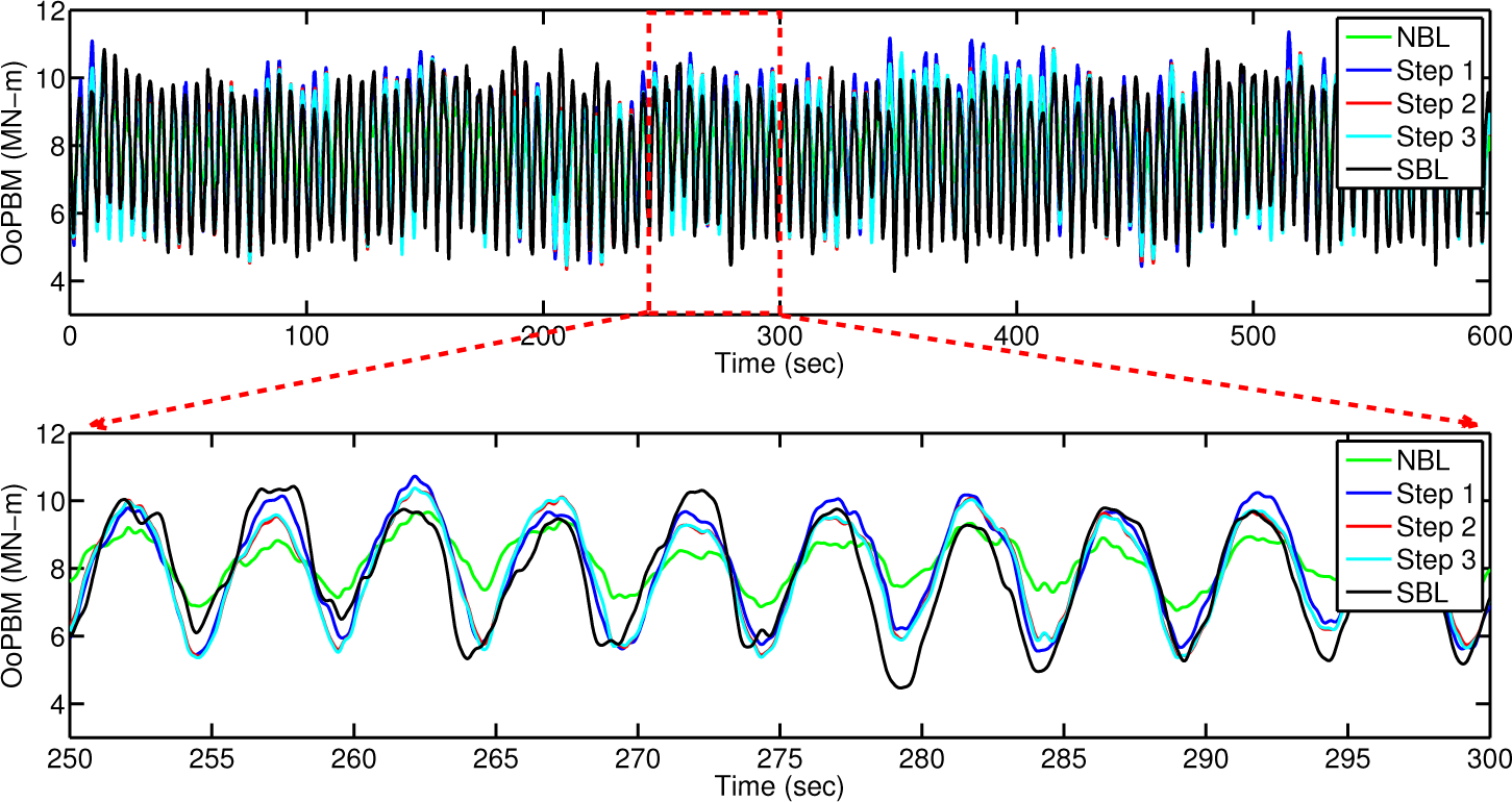
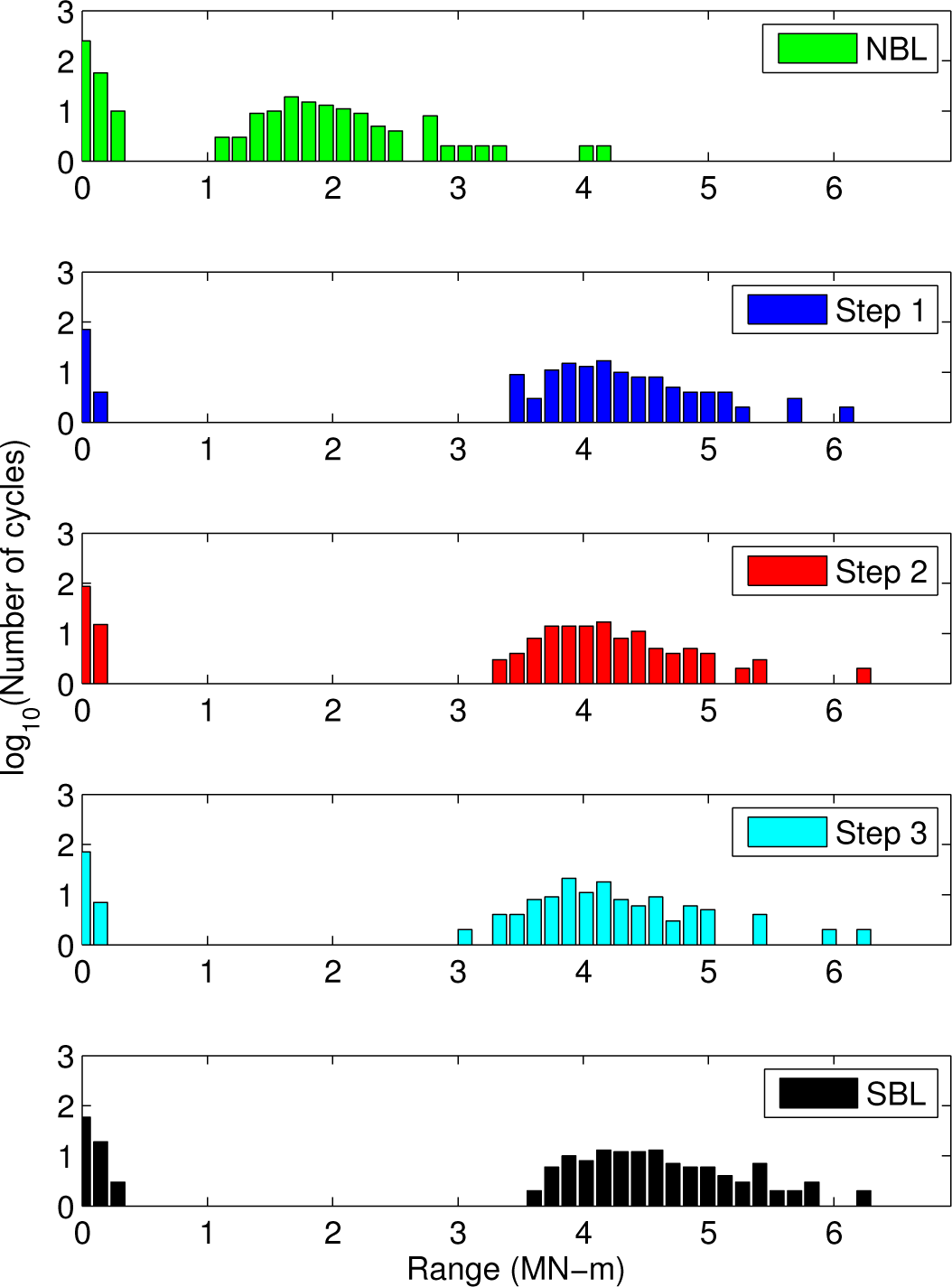
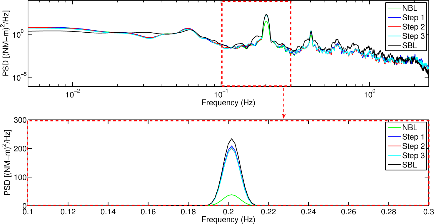
Figure 8 compares OoPBM time series for the various cases, all represented by different color lines; the top plot is a 10-min time series while the bottom one is for a 50-s segment. Figure 9 compares OoPBM power spectra for the various cases; the top plot is for a wider frequency range while the bottom one is for a narrow range and is plotted using a linear scale. In general, the OoPBM based on the SBL wind field (black line) exhibits stronger periodic behavior than the other cases; it is more narrow-banded. The shear-enhancing modification in Step 1 makes a significant correction to the baseline NBL case by increasing OoPBM amplitudes as can be seen in the increased power spectrum peak. Subsequent modifications from Steps 2 and 3 do not significantly change the OoPBM process. Figure 10 compares OoPBM range histograms (from rainflow cycle counting) for the various cases where it is seen even more clearly that the Step 1 modification, which enhances the shear in the baseline NBL flow field, leads to a very similar range histogram to that for the SBL case; again Steps 2 and 3 do not significantly add to the adjustment after Step 1.
3.3.2. Tower-Top Yawing Moment
Figure 11 compares TTYM time series and Figure 12 compares TTYM power spectra for the various cases. The Step 1 (shear-enhancing) modification to the baseline NBL flow field increases both the mean value and the amplitude of the TTYM process. The increased amplitude is clear from the increased energy seen over a range of frequencies in the PSD plot. The Step 2 mean wind direction correction to the NBL flow further increases the amplitude of the TTYM process, making the time series and PSD plots more comparable to those for the SBL case. The TTYM process appears to be influenced by both wind shear and wind direction variation over the rotor-swept area. Figure 13 compares TTYM range histograms for the various cases. Step 1 increases the number of some high-amplitude cycles; Step 2 makes slight additional corrections to the histograms. Even after all three steps of modification (accounting for vertical profile matching in wind shear, wind direction, and turbulence standard deviation), the TTYM histograms are still quite different compared to the histogram for the SBL case, which has significantly more high-amplitude cycles. This deviation in TTYM range histograms, which influence fatigue loads, is investigated further by comparing the baseline and adjusted NBL fields and the SBL fields in some detail next.
Figure 14 shows the variation with time and space (over the rotor-swept area) of the longitudinal turbulence in the NBL and SBL flow fields and their impact on TTYM loads, which are compared in the bottom plot. We extracted ≈20-second segments of the TTYM time series from the two cases where deviations were especially large and then compared turbulence levels during that period. The mean wind fields are the same in the two cases; therefore, the contrasting variation in turbulence for the two cases is the reason the TTYM process for the SBL case has higher load amplitudes. Studying the 3-D turbulence distribution plots, it is seen that the SBL wind field has more locally concentrated (coherent) and organized turbulence structures. These turbulence structures are sustained for a while, during which time the corresponding TTYM process cyclic amplitudes are large. Such locally concentrated turbulence causes strong asymmetric forces on the rotor and, in turn, brings about large tower-top yawing moments, TTYM, that are enhanced by these asymmetric loading effects.
3.3.3. Fore-Aft Tower Base Moment
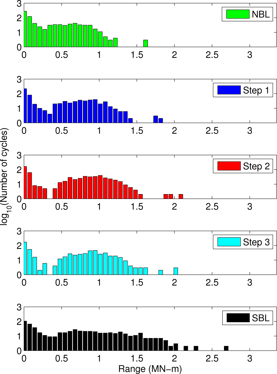
Figure 15 compares FATBM time series and Figure 16 compares power spectra for the various cases. In contrast with the blade loads, there is greater influence of low-frequency energy on the FATBM process and greater differences between the SBL and NBL wind fields (baseline and adjusted) in that low-frequency range. Because the SBL wind fields have lower energy in the low-frequency region, the FATBM process also has lower energy levels there for SBL flow fields relative to that for the other flow fields. Figure 17 compares FATBM range histograms for the SBL and NBL cases. The low-amplitude cycles (or ranges) in the histogram are somewhat smaller in number for the SBL wind field compared to that for the baseline NBL and the adjusted wind fields; this is because the SBL wind fields have reduced turbulence energy at high frequencies that are responsible for the low-amplitude load cycles. We shall see later that differences in these small-amplitude cycle counts do not greatly influence fatigue loads on the tower. The FATBM range histogram shows smaller differences among the different flow fields for the large-amplitude cycles.
4. Comparison of Time-Varying Wind-Related Processes and Wind Turbine Load Processes
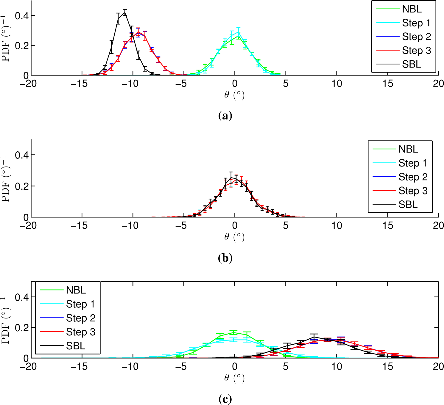
We examine next how the probability distributions of processes describing the longitudinal wind velocity, U, the lateral wind velocity, V, and the wind direction, θ, compare for the baseline NBL wind field, the modified wind fields, and the SBL wind field. We examine these various processes at different elevations including the top, center (hub), and bottom of the rotor-swept area. Probability density functions (PDFs) will be accordingly studied first for U, V, and θ. After this, we compare PDFs for the three load processes (OoPBM, TTYM, and FATBM) for the various wind fields.
4.1. Wind Field Process
Figure 18 compares PDFs for the longitudinal wind velocity time series at three locations—the rotor top (top of the rotor-swept area), the rotor hub, and the rotor bottom (bottom of the rotor-swept area). The PDFs are based on averages from five wind fields extracted from the last stage (twelfth hour of the LES run) for the LES control case and from the corresponding matched NBL baseline and modified wind fields. Error bars indicate one sample standard deviation on each indicated PDF ordinate. Step 1 (with enhanced shear to the baseline NBL flow) is seen to move the PDF for U, at the rotor top, towards higher wind speeds and, at the rotor bottom, towards lower wind speeds. Not much change results at the rotor hub since Uh and σU were matched there for the SBL and baseline NBL cases. Step 2 results in no change to the PDFs for U since it mainly influences the lateral velocity, V. Step 3, which suppresses turbulence at the top and enhances it at the bottom, causes the PDF to get narrower at the rotor top and wider at the rotor bottom. We note that the PDFs for U for the NBL-adjusted wind fields get more and more similar to that for the SBL field with each modification step to the base NBL flow.
Figure 19 compares PDFs for the lateral wind velocity time series at the same three locations as before. Steps 1 and 3 do not affect the PDF for V because they only modify the longitudinal wind velocity, U. Step 2 (adjusting for wind direction variation with height), however, has an effect on the PDF for V at the rotor top and bottom as expected. This is the result of introducing a non-zero mean lateral velocity component, , to the baseline NBL wind field. We see that Step 2 effectively modifies the PDF for V so that it is more similar to that of the SBL wind field than was the case with the baseline NBL wind field.
Figure 20 compares PDFs for the wind direction time series at the same three locations as before. Step 1 does not significantly alter the PDF for θ; it slightly widens the PDF at the rotor bottom due to adjustments to the mean longitudinal wind speed there. Step 2 significantly modifies the PDF for θ so that it closely resembles that for the SBL wind field. The small differences between the PDFs from the NBL-modified (Step 3) wind field and the SBL wind field are due to the approximated linear variation assumed for the mean wind direction profile. Step 3 has little effect on the PDF for θ because although the longitudinal turbulence is scaled, it is relatively very small compared to U to influence the time-varying wind direction to any great extent.
4.2. Comparison of Wind Turbine Load Processes
We compare PDFs of wind turbine load processes for the baseline NBL wind field, the modified wind fields, and the SBL wind field in order to assess the influence of SBL wind field characteristics related to wind shear, wind veer, and turbulence gradients. Again, we average PDF curves estimated from five wind fields generated from the twelfth hour of the LES-SBL control case. Similarly, we obtain averaged PDF curves for the baseline NBL wind field and for the step-wise modified wind fields. a comparison of these PDF curves enables us to assess the effect of each SBL-associated wind field characteristic on the load processes. In this comparison exercise, we use the same wind fields that were used in the time-varying wind-related process PDF comparisons (summarized in Figures 18–20). Figures 21–23 present PDFs for three different turbine load processes—the blade-root out-of-plane bending moment (OoPBM), the tower-top yawing moment (TTYM), and the base fore-aft tower bending moment (FATBM).
4.2.1. Blade Root Out-of-Plane Bending Moment
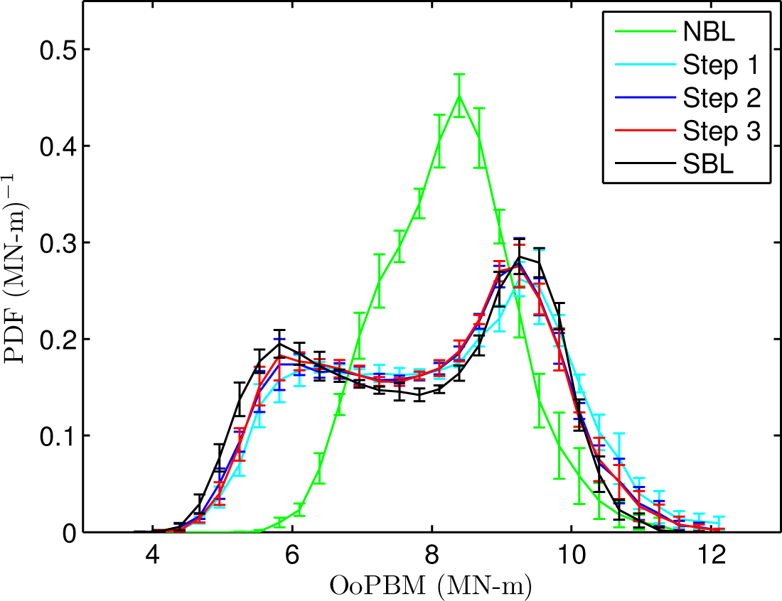
Figure 21 compares OoPBM PDFs. We note that the shape of the PDF for the baseline NBL wind field is completely different from that for the SBL wind field. However, the three modification steps cause the resulting wind field to produce an OoPBM PDF that is quite similar to that resulting from the SBL wind field. Step 1 changes the uni-modal PDF to a bimodal one; the difference in the load levels at the two modes represents a dominant amplitude of the load process. This suggests that enhancing of the wind shear changes the OoPBM from a broad-banded process to a somewhat more narrow-banded one with a stronger periodic component. This trend can be verified in the OoPBM time series (Figure 8) which show increases in the OoPBM process amplitude, and in the PSD plots (Figure 9) which show that the 1P (1 per rev) energy peak is significantly increased with the Step 1 shear enhancement. Note that the asymmetry in the PDF curve results from the different wind velocity variation that a blade experiences when it rotates in the upper half of the rotor plane versus in the lower half. Velocity differences between the rotor hub and bottom are larger than those between the rotor hub and top due to the power-law shear profile; this causes an asymmetric periodic OoPBM process and, also, an asymmetric PDF. Steps 2 and 3 lead to somewhat smaller adjustments to the OoPBM PDF. In summary, by merely enhancing the wind shear, OoPBM loads from the NBL wind field become quite similar to those from the SBL wind field.
4.2.2. Tower-Top Yawing Moment
Figure 22 compares TTYM PDFs. The Step 1 modification to the baseline NBL wind field shifts the TTYM PDF curve towards larger load levels and moves the mode and mean TTYM closer to those for the SBL wind field. Steps 2 and 3 have little apparent influence on the PDF for TTYM. Even after all the flow field modifications, there are still deviations in the TTYM PDF curve relative to that from the SBL wind field whose PDF has a more significant upper tail; these larger TTYM values are associated with larger amplitude cycles. Fatigue of the nacelle yaw bearing will likely be influenced by these large-amplitude TTYM cycles. The differences in the PDFs for the NBL-modified wind fields and the SBL wind field arise, at least in part, from localized and sustained turbulent structures that cause highly asymmetric forces over the turbine rotor plane that drive the TTYM process.
4.2.3. Base Fore-Aft Tower Bending Moment
Figure 23 compares FATBM PDFs. The PDF for the baseline NBL wind field has a more significant upper tail compared to that for the SBL wind field. Step 1 moves the FATBM PDF in the opposite direction instead of approaching the PDF for the SBL wind field. Steps 2 and 3 reverse this trend to some degree but there still remains a significant difference in the FATBM PDFs for the NBL-modified wind fields versus the SBL wind field. It is worth noting that, on a relative scale, the deviations in the FATBM are not very large compared to the mean or center of the FATBM PDF; we note that the deviation in the TTYM loads were significantly larger relative to the mean TTYM value.
5. Extreme and Fatigue Load Statistics
The entire suite of 2200 SBL wind fields generated from 44 LES runs is considered next. The same procedure described for the single control case is now repeated for all of the 2200 wind fields. Thus, baseline NBL wind fields are first generated with matching mean wind speed and standard deviation values at hub height as were found for the SBL wind fields. Then, necessary modifications are made in three steps where vertical profiles of the mean wind speed, mean wind direction, and turbulence standard deviation are modified as discussed before. Figure 24 shows a schematic flow chart that explains the procedure adopted for assessing the influence of SBL-related wind field characteristics on wind turbine loads.
5.1. A Comparison of Wind Field Variables’ Contributions to Load Statistics
Equivalent fatigue load (EFL) estimates and 10-min extreme (Max) load estimates for each 10-min time series are used to compare each wind field variable’s contribution and importance. (Note that an “equivalent fatigue load” or EFL is defined such that a fixed number of stress cycles—here, we consider 1000—of amplitude, EFL, result in the same damage as that found by the actual number of variable-amplitude stress cycles in each load 600-s time series analyzed.) These two load statistics are compared for inflow fields defined based on 2200 wind fields generated from the 44 LES-SBL runs, for 2200 baseline NBL wind fields generated stochastically using TurbSim based on the IEC standard, and for each of three sets of 2200 modified NBL wind fields with internal variable matching steps. We compare these load statistics in different flow regimes (as defined in Section 1.3) defined according to the relative importance of shear and turbulence; this is done to evaluate the contribution of each wind field internal variable on turbine loads in each regime. This type of comparison provides some insight into how extreme and fatigue load statistics are affected by the level of turbulence and shear.
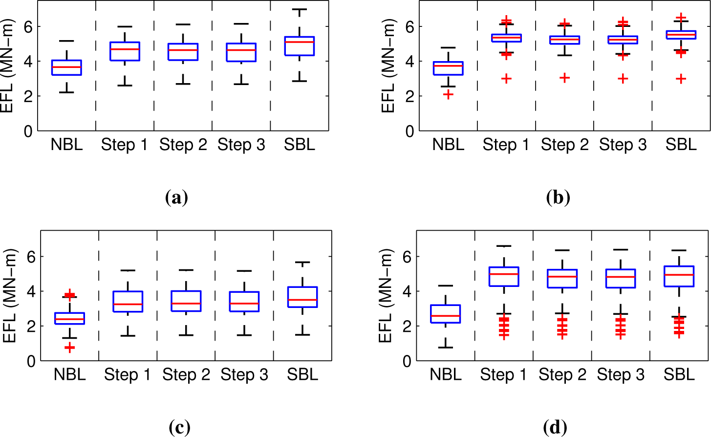
Figures 25–30 compare equivalent fatigue load (EFL) values and 10-min maximum loads from time series of OoPBM, TTYM and FATBM. We compare these load statistics for four different flow regimes: (a) weak shear and strong turbulence (zα < 0 & zσ > 0); (b) strong shear and strong turbulence (zα > 0 & zσ > 0); (c) weak shear and weak turbulence (zα < 0 & zσ < 0); and (d) strong shear and weak turbulence (zα > 0 & zσ < 0). Box plots in each of these four groups summarize the median value (red line), the 25% and 75% fractiles (boundary of blue box), and the minimum and maximum values (extended black bars) for the EFL and 10-min maximum values for loads evaluated for wind fields from the available 2200 that are contained in that group. The red crosses represent outliers.
5.1.1. Blade-Root Out-of-Plane Bending Moment
Figure 25 compares EFL statistics for OoPBM. Step 1 (wind shear enhancing) significantly increases the median EFL, making this case comparable to the SBL case. This improvement is especially evident in the strongly stratified (stable) groups, (b) and (d). The other modification steps affect the EFL for OoPBM only very slightly. Thus, correct representation of wind shear in the stable boundary layer is critical to estimate OoPBM fatigue loads. Figure 26 compares statistics of the 10-min maximum OoPBM. Each modification step has a small influence on the maximum load; Step 1 slightly increases the median of the 10-min maximum load, and this increased median is comparable to that for the SBL case. The small changes are because maximum values are not sensitive to modifications (in the three steps) that are made to the entire load process but are affected mostly by instantaneous large values. Such instantaneous effects are correlated more strongly with the level of turbulence; hence, the strong turbulence regimes, (a) and (b), are associated with larger maximum loads than the weaker turbulence regimes, (c) and (d).
5.1.2. Tower-Top Yawing Moment
Figure 27 compares EFL statistics for TTYM. Each modification step gradually increases the EFL values; however, the median EFL for the SBL wind field is still much higher than that for the baseline NBL and the modified wind fields. In the more stable cases, (b) and (d), the effects of each modification are more apparent because enhanced wind shear and wind veer (that influence TTYM) are more significant in these cases and, thus, the mean wind fields in these regimes are modified more significantly compared with the other cases. In the weakly stable cases, (a) and (c), we notice small improvements with modifications to the baseline NBL winds and large differences relative to the SBL winds. This suggests that some other factor in the SBL wind field, that is not accounted for in our stochastic NBL field modifications, possibly contributes to TTYM fatigue loads. We saw earlier that these TTYM EFL deviations for stochastic NBL versus LES-SBL wind fields are likely caused by contrasting spatial and temporal turbulence structures. Figure 28 compares statistics of the 10-min maximum TTYM. The variation in statistics for the 10-min maximum TTYM in each case is similar to that seen for the EFL. It is important to point out that the large TTYM values seen with the SBL wind fields cannot be estimated by stochastic simulation, even if modifications for wind shear, veer, and turbulence variation over the rotor plane are taken into consideration (i.e., after all the modifications to the baseline NBL wind field have been applied).
5.1.3. Fore-Aft Tower Base Moment
Figures 29 and 30 compare statistics for the EFL and 10-min maximum values, respectively, of the FATBM process. Both EFL and 10-min maximum values for FATBM corresponding to the baseline NBL wind field are already comparable to those for the SBL wind field; this suggests that the hub-height mean wind speed and turbulence standard deviation alone, i.e., Uh and σU, are sufficient to predict EFL and 10-min maximum values of FATBM, regardless of atmospheric stability conditions. This trend can also be seen by comparing load statistics in the weakly stable cases, (a) and (c), with those in the more strongly stable cases, (b) and (d). The median values for the EFL and 10-min maxima do not vary with change in the degree of stability but show some variation with the level of turbulence; the median EFL values and 10-min maxima are significantly larger in the strongly turbulent regimes, (a) and (b). This can be simply explained by the “cantilever” analogy for this tower base moment—fluctuations in wind speed cause fluctuations in the forces exerted at the wind turbine tower top which, in turn, lead to overturning moment variations at the tower base. In this manner, the wind turbine’s hub height of 90 m acts as a moment arm, converting enhanced wind speed fluctuations (turbulence) to significantly amplified FATBM levels.
5.2. Summary on Load Statistics
Table 3 summarizes the comparison of EFL statistics for all three wind turbine loads, OoPBM, TTYM and FATBM, based on the 2200 SBL fields and associated baseline and modified NBL wind fields. The mean and standard deviation of the EFL values are presented. First, for the OoPBM case, Step 1 is seen to increase the mean EFL by almost 50% compared to the baseline NBL wind field; also, this increased mean value is almost comparable to that for the SBL case. The standard deviation of the OoPBM EFL value is not significantly affected by modifications to the baseline NBL wind field. Second, for the TTYM case, though each step of modification of the baseline NBL field slightly changes the mean EFL, these values never reach the same level as seen for the SBL wind field. As mentioned before, this deviation between baseline NBL (even after internal variable modifications) and SBL wind fields is because of contrasting characteristics of the turbulence fields such as in the coherence and local energy distribution over the rotor plane. Finally, for the FATBM case, the mean EFL is seen to be relatively unchanging for the baseline NBL and modified wind fields and it is comparable with that for the SBL wind field. This is because the base fore-aft tower bending moment is influenced primarily by the longitudinal mean wind speed and turbulence standard deviation, both of which are matched for the stochastic NBL and LES-SBL cases. The complex interaction between the blades and inflow wind field characteristics such as shear, wind direction, and turbulence variation over the rotor does not appear to greatly affect loads at the tower base.
Table 4 summarizes statistics on ten-minute maximum values for OoPBM, TTYM, and FATBM, based on the 2200 SBL wind fields and associated baseline and modified NBL wind fields. The mean and standard deviation of the 10-min maximum values are presented. First, for the OoPBM case, the mean of the 10-min maximum values is similar for all the simulated wind fields. The 10-min maximum load appears to be most directly influenced by the hub-height mean wind speed, Uh, and standard deviation, σU, and all the wind field cases share these same values of Uh and σU. Second, for the TTYM case, Step 1 significantly increases the mean of the 10-min maximum TTYM. We saw before how an enhanced wind shear leads to an increase in the overall load level for TTYM. Thus, the Step 1 modification helps to make the maximum TTYM closer to that from the SBL wind field. Note, however, that the mean 10-min maximum TTYM for the SBL case is still considerably larger that those for the baseline NBL and the other wind fields, even after all the modifications. Finally, for the FATBM case, the mean of the 10-min maximum shows a similar trend to that for the OoPBM; the mean and standard deviation values of the maximum TTYM are similar for the SBL and all the other wind fields. This, again, suggests that the maximum base fore-aft tower bending moment is primarily influenced by the hub-height mean wind speed and standard deviation, Uh and σU.
5.3. Summary on Differences in the LES-SBL, Stochastic-NBL, and Modified Wind Fields
We finally seek to understand trends between the wind field conditions, grouped into four regimes based on relative levels of shear and turbulence, and estimated SBL-related wind field characteristics such as the enhanced wind shear, the wind direction difference between the rotor top and bottom (Δθ = Ŝθ · Drotor where Drotor is the rotor diameter), and the standard deviation difference between the rotor top and bottom (Δσ = Ŝσ · Drotor). Table 5 provides statistics on those estimated parameters; we use the 25- and 75-percentile values, Q1 and Q3, to assess the extent of variation in these different wind field characteristics where the number of data sets varies for each of the four groups. In general, the values of , Δθ, and Δσ are all higher when shear is strong, i.e., when zα > 0, which is the case for strongly stratified (stable) conditions.
We have focused on three SBL-related wind field characteristics and attempted to include them stochastically in modifications to baseline NBL wind fields. For all the SBL and NBL wind fields, we estimated EFL and 10-min maximum loads for OoPBM, TTYM and FATBM. The percent differences in these load statistics estimated by SBL and the baseline NBL wind fields are presented. The negative differences seen in so many of the load statistics suggest that, in general, the baseline NBL wind fields underestimate load statistics compared to the SBL case. In particular, the EFL for OoPBM and both the EFL and 10-min maximum for TTYM are grossly underestimated; the differences are most severe when the wind shear is strong (zα > 0).
All three of the wind field modifications are applied to the baseline NBL wind fields in Step 3; therefore, by investigating percentile differences in the load statistics estimated from SBL and the modified wind fields after Step 3, we can learn about the cumulative importance of the three wind field characteristics (wind shear, wind direction, and turbulence variation) on loads. Also, the previously provided percentile differences on loads between the SBL and baseline NBL case provide a useful reference for this comparison. After three steps of modification to the baseline NBL wind fields, the percent differences in load statistics relative to the NBL case have, in general, decreased; this suggests that although the stochastically generated modified wind fields still underestimate loads, the wind field characteristics modified successively in the baseline NBL fields do have some influence on the turbine loads. In particular, the EFL for OoPBM under strongly stable conditions is greatly improved; in the strong shear and weak turbulence regime, the percentile difference (Q1; Q3) range changed from (−51.9; −39.0) to (−4.6; 0.3). In the case of TTYM, such improvements are slight and not as significant.
The percent differences (SBL versus other wind fields) in 10-min load maxima are smaller than those in EFL values and they do not show clear great advantages of wind field modifications in matching SBL load statistics. This is because maximum values are most related to turbulence and wind speed rather than to wind shear and mean wind direction profiles. Still, in the case of TTYM, percent errors are reduced after modification to the baseline NBL wind field, particularly when the wind shear is strong; this appears to be due to the increased mean values of TTYM that result from the enhanced wind shear. The significant difference in TTYM loads in the SBL and baseline NBL wind fields is an interesting topic for further study; SBL conditions clearly cause these loads to be higher.
6. Discussion and Conclusions
SBL and NBL wind fields were compared by studying characteristics of these contrasting wind fields and associated loads on a 5-MW wind turbine. Large-eddy simulation is capable of generating more realistic and physical wind inflow fields by accounting for atmospheric stability. The major qualitative differences in pertinent turbine-scale flow characteristics derived from SBL and NBL wind fields are summarized in Table 6.
To isolate SBL-related wind field characteristics and their influence on wind turbine loads, we attempted modifications of baseline NBL wind fields generated by stochastic simulation so as to match the turbine-scale wind field characteristics of the SBL wind fields. Statistics and probability distributions for the stochastically modified wind fields and the SBL wind fields were compared and it was generally found that modifications yielded flow characteristics and load statistics that more closely resembled the SBL case in contrast to when the baseline NBL case was considered in similar comparison. Each load type for the wind turbine selected was differently affected by the SBL-related wind field characteristics. By studying fatigue and extreme load statistics (EFL and 10-min maxima) for different load types, we evaluated the contribution of separate wind field characteristics (related to shear, veer, and turbulence) to rotor and tower wind turbine loads. The results are summarized as follows:
The EFL and 10-min maximum values for the blade root out-of-plane bending moment (OoPBM) are mainly influenced by Uh and σU. In the case of the EFL, wind shear had especially significant effect.
The EFL and 10-min maximum values for the tower-top yawing moment (TTYM) are significantly influenced by spatially and temporally organized turbulence structures that are evident only in the LES-SBL flows but are difficult to include in a purely stochastic wind field simulation approach, even if turbine-scale modifications are made for shear, veer, and turbulence variation across the rotor.
The EFL and 10-min maximum values for the base fore-aft moment tower bending moment are mainly influenced by Uh and σU. As such, SBL-specific characteristics such as wind shear and veer are of secondary importance.
In summary, this study sought to investigate if one could reproduce wind field characteristics associated with the stable boundary layer by using simpler stochastic simulation approaches by making appropriate corrections, when necessary, for shear, veer, turbulence, etc. evident in LES-generated SBL flows. We note that simple tuning of this kind, in general, cannot consistently match turbine load statistics, even if this is possible in some cases. This finding is significant in that it suggests that accurate representation of conditions in the stable boundary layer requires LES and that design approaches that favor the use of simpler stochastic simulation, believed to be acceptable for neutral boundary layer conditions, cannot easily be modified to capture SBL-specific flow field features.
Acknowledgments
The authors acknowledge the financial support received from the National Science Foundation (NSF) by way of Grant Nos. CBET-0967816, CBET-1050806, and AGS-1122315. Any opinions, findings, and conclusions or recommendations expressed in this material are those of the authors and do not necessarily reflect the views of the sponsor.
Author Contributions
The first author prepared a draft of this manuscript and performed all the stochastic simulations as part of his Master’s thesis; he also analyzed the large-eddy simulations that were generated by the third author. The second and third authors made significant contributions and provided important insights to the study and to the initial written draft; the second author also served as supervisor of the first author’s thesis research and provided the motivation, guidance, and direction for the entire study as presented.
Conflicts of Interest
The authors declare no conflict of interest.
References
- Sim, C. Simulation and Anlysis of Wind Turbine Loads for Neutrally Stable Inflow Turbulence. M.S. Thesis, University of Texas at Austin, Austin, TX, USA, 2009. [Google Scholar]
- Sim, C.; Basu, S.; Manuel, L. The influence of stable boundary layer flows on wind turbine fatigue loads, Proceedings of the 47th AIAA Aerospace Sciences Meeting Including the New Horizons Forum and Aerospace Exposition, Paper No. AIAA 2009–1405, Orlando, FL, USA, 5–8 January 2009.
- Sim, C.; Basu, S.; Manuel, L. On space-time resolution of inflow representations for wind turbine Loads Analysis. Energies 2012, 5, 2071–2092. [Google Scholar]
- Park, J.; Basu, S.; Manuel, L. Large-eddy simulation of stable boundary layer turbulence and estimation of associated wind turbine loads. Wind Energy 2014, 17, 359–384. [Google Scholar]
- International Electrotechnical Commission (IEC), Wind Turbine Generator System Part 1: Design Requirements, 3rd ed.; IEC: Geneva, Switzerland, 2005, IEC 61400-1.
- Kelley, N.D. A Case for Including Atmospheric Thermodynamic Variables in Wind Turbine Fatigue Loading Parameter Identification; Technical Report NREL/CP-500-26829; National Renewable Energy Laboratory: Golden, CO, USA, 1999. [Google Scholar]
- Hand, M.M.; Kelley, N.D.; Balas, M.J. Identification of Wind Turbine Responses to Turbulent Inflow Structures; Technical Report NREL/CP-500-33465; National Renewable Energy Laboratory: Golden, CO, USA, 2003. [Google Scholar]
- Kelley, N.; Shirazi, M.; Jager, D.; Wilde, S.; Adams, J.; Buhl, M.; Sullivan, P.; Patton, E. Lamar Low-Level Jet Project Interim Report; Technical Report NREL/TP-500-34593; National Renewable Energy Laboratory: Golden, CO, USA, 2004. [Google Scholar]
- Basu, S.; Foufoula-Georgiou, E.; Porté-Agel, F. Synthetic turbulence, fractal Interpolation, and large-eddy simulation. Phys. Rev. 2004, 70, 026310. [Google Scholar]
- Jonkman, B.J.; Buhl, M.L. TurbSim User’s Guide; Technical Report NREL/EL-500-41136; National Renewable Energy Laboratory: Golden, CO, USA, 2007. [Google Scholar]
- Basu, S.; Porté-Agel, F. Large-eddy simulation of stably stratified atmospheric boundary layer turbulence: A scale-dependent dynamic modeling approach. J. Atmos. Sci. 2006, 63, 2074–2091. [Google Scholar]
- Jonkman, J.M.; Buhl, M.L. FAST User’s Guide; Technical Report NREL/EL-500-38230; National Renewable Energy Laboratory: Golden, CO, USA, 2005. [Google Scholar]
- Jonkman, J.M.; Butterfield, S.; Musial, W.; Scott, G. Definition of a 5 MW Reference Wind Turbine for a Offshore System Development; Technical Report NREL/TP-500-38060; National Renewable Energy Laboratory: Golden, CO, USA, 2007. [Google Scholar]
- Brown, A.R.; Derbyshire, S.H.; Mason, P.J. Large-eddy simulation of stable atmospheric boundary layers with a revised stochastic subgrid model. Quart. J. Roy. Meteor. Soc. 1994, 120, 1485–1512. [Google Scholar]
- Saiki, E.M.; Moeng, C.H.; Sullivan, P.P. Large-eddy simulation of the stably stratified planetary boundary layer. Bound. Layer Meteorol 2000, 95, 1–30. [Google Scholar]
- Jiménez, M.A.; Cuxart, J. Large-eddy Simulations of the Stable Boundary Layer Using the Standard Kolmogorov Theory: Range of Applicability. Bound. Layer Meteor 2005, 115, 241–261. [Google Scholar]
- Basu, S.; Holtslag, A.A.M.; van de Wiel, B.J.H.; Moene, A.F.; Steeneveld, G.J. An inconvenient “truth” about using sensible heat flux as a surface boundary condition in models under stably stratified regimes. Acta Geophys 2008, 56, 88–99. [Google Scholar]
- Basu, S.; Vinuesa, J.F.; Swift, A. Dynamic LES modeling of a diurnal cycle. J. Appl. Meteorol. Climatol. 2008, 47, 1156–1174. [Google Scholar]
- Beare, R.J.; Macvean, M.K. Coauthors. An intercomparison of large-eddy simulations of the stable boundary layer. Bound. Layer Meteorol 2006, 118, 247–272. [Google Scholar]
- Yamada, T.; Mellor, G. A simulation of the Wangara atmospheric boundary layer data. J. Atmos. Sci. 1975, 32, 2309–2329. [Google Scholar]
- Basu, S.; Holtslag, A.A.M.; Bosveld, F.C. GABLS3 LES Intercomparison Study, Proceedings of the ECMWF/GABLS Workshop on “Diurnal cycles and the stable atmospheric boundary layer”, Reading, UK, 7–10 November 2011; pp. 75–82.
- Zhou, B.; Chow, F.K. Large-eddy simulation of the stable boundary layer with explicit filtering and reconstruction turbulence modeling. J. Atmos. Sci. 2011, 68, 2142–2155. [Google Scholar]


| No. | G (m-s−1) | C (K-h−1) | z0 (m) | Hi (m) | N (K-m−1) | f (s−1) | DG (m-s−1) |
|---|---|---|---|---|---|---|---|
| 1 | 9 | 0.75 | 0.03 | 200 | 0.003 | 0.00010 | 0 |
| 2 | 12 | 0.75 | 0.01 | 200 | 0.003 | 0.00010 | 0 |
| 3 | 12 | 0.75 | 0.03 | 200 | 0.003 | 0.00010 | 0 |
| 4 | 12 | 0.75 | 0.03 | 300 | 0.003 | 0.00010 | 0 |
| 5 | 12 | 2.00 | 0.03 | 200 | 0.003 | 0.00010 | 0 |
| 6 | 15 | 0.50 | 0.03 | 200 | 0.003 | 0.00010 | 0 |
| 7 | 15 | 0.75 | 0.01 | 200 | 0.003 | 0.00010 | 0 |
| 8 | 15 | 0.75 | 0.01 | 200 | 0.003 | 0.00012 | 0 |
| 9 | 15 | 0.75 | 0.03 | 50 | 0.003 | 0.00010 | 0 |
| 10 | 15 | 0.75 | 0.03 | 100 | 0.003 | 0.00010 | 0 |
| 11 | 15 | 0.75 | 0.03 | 200 | 0.003 | 0.00008 | 0 |
| 12 (CONTROL) | 15 | 0.75 | 0.03 | 200 | 0.003 | 0.00010 | 0 |
| 13 | 15 | 0.75 | 0.03 | 200 | 0.003 | 0.00010 | 2 |
| 14 | 15 | 0.75 | 0.03 | 200 | 0.003 | 0.00010 | 4 |
| 15 | 15 | 0.75 | 0.03 | 200 | 0.003 | 0.00010 | 6 |
| 16 | 15 | 0.75 | 0.03 | 200 | 0.003 | 0.00010 | 8 |
| 17 | 15 | 0.75 | 0.03 | 200 | 0.003 | 0.00012 | 0 |
| 18 | 15 | 0.75 | 0.03 | 200 | 0.010 | 0.00008 | 0 |
| 19 | 15 | 0.75 | 0.03 | 200 | 0.010 | 0.00010 | 0 |
| 20 | 15 | 0.75 | 0.03 | 200 | 0.010 | 0.00012 | 0 |
| 21 | 15 | 0.75 | 0.03 | 300 | 0.003 | 0.00010 | 0 |
| 22 | 15 | 0.75 | 0.10 | 200 | 0.003 | 0.00010 | 0 |
| 23 | 15 | 0.75 | 0.10 | 200 | 0.003 | 0.00012 | 0 |
| 24 | 15 | 1.00 | 0.03 | 200 | 0.003 | 0.00010 | 0 |
| 25 | 15 | 1.00 | 0.10 | 200 | 0.003 | 0.00008 | 0 |
| 26 | 15 | 1.00 | 0.10 | 200 | 0.003 | 0.00012 | 0 |
| 27 | 15 | 1.25 | 0.03 | 200 | 0.003 | 0.00010 | 0 |
| 28 | 15 | 1.50 | 0.03 | 200 | 0.003 | 0.00010 | 0 |
| 29 | 15 | 2.00 | 0.03 | 200 | 0.003 | 0.00010 | 0 |
| 30 | 18 | 0.75 | 0.01 | 200 | 0.003 | 0.00010 | 0 |
| 31 | 18 | 0.75 | 0.03 | 50 | 0.003 | 0.00010 | 0 |
| 32 | 18 | 0.75 | 0.03 | 100 | 0.003 | 0.00010 | 0 |
| 33 | 18 | 0.75 | 0.03 | 200 | 0.003 | 0.00010 | 0 |
| 34 | 18 | 0.75 | 0.03 | 200 | 0.003 | 0.00010 | 2 |
| 35 | 18 | 0.75 | 0.03 | 200 | 0.003 | 0.00010 | 4 |
| 36 | 18 | 0.75 | 0.03 | 200 | 0.003 | 0.00010 | 6 |
| 37 | 18 | 0.75 | 0.03 | 200 | 0.003 | 0.00010 | 8 |
| 38 | 18 | 0.75 | 0.03 | 200 | 0.010 | 0.00010 | 0 |
| 39 | 18 | 0.75 | 0.03 | 300 | 0.003 | 0.00010 | 0 |
| 40 | 18 | 0.75 | 0.10 | 200 | 0.003 | 0.00010 | 0 |
| 41 | 18 | 1.00 | 0.03 | 200 | 0.003 | 0.00010 | 0 |
| 42 | 18 | 1.25 | 0.03 | 200 | 0.003 | 0.00010 | 0 |
| 43 | 18 | 1.50 | 0.03 | 200 | 0.003 | 0.00010 | 0 |
| 44 | 18 | 2.00 | 0.03 | 200 | 0.003 | 0.00010 | 0 |
| NBL | Step 1 | Step 2 | Step 3 | SBL | |
|---|---|---|---|---|---|
| Uh (m/s) | 12.288 | 12.288 | 12.288 | 12.288 | 12.304 |
| σU (m/s) | 0.392 | 0.392 | 0.392 | 0.392 | 0.412 |
| 0.417 | 0.417 | 0.417 | 0.417 | ||
| Ŝθ(°/m) | −0.136 | −0.136 | −0.136 | ||
| Ŝσ ((m/s)/m) | [−0.0024, −0.0023] | [−0.0024, −0.0023] |
| OoPBM | |||||
|---|---|---|---|---|---|
| NBL | Step 1 | Step 2 | Step 3 | SBL | |
| μ (MN-m) | 3.10 | 4.56 | 4.49 | 4.49 | 4.75 |
| σ (MN-m) | 0.81 | 0.95 | 0.89 | 0.90 | 0.96 |
| TTYM | |||||
| NBL | Step 1 | Step 2 | Step 3 | SBL | |
| μ (MN-m) | 1.42 | 1.60 | 1.73 | 1.77 | 2.33 |
| σ (MN-m) | 0.36 | 0.33 | 0.38 | 0.35 | 0.41 |
| FATBM | |||||
| NBL | Step 1 | Step 2 | Step 3 | SBL | |
| μ (MN-m) | 6.83 | 6.91 | 6.96 | 6.66 | 6.87 |
| σ (MN-m) | 2.92 | 2.94 | 2.83 | 2.83 | 2.70 |
| OoPBM | |||||
|---|---|---|---|---|---|
| NBL | Step 1 | Step 2 | Step 3 | SBL | |
| μ (MN-m) | 10.37 | 11.10 | 10.94 | 10.85 | 10.82 |
| σ (MN-m) | 1.40 | 1.37 | 1.33 | 1.33 | 1.41 |
| TTYM | |||||
| NBL | Step 1 | Step 2 | Step 3 | SBL | |
| μ (MN-m) | 1.44 | 1.93 | 1.97 | 2.06 | 2.56 |
| σ (MN-m) | 0.41 | 0.40 | 0.38 | 0.43 | 0.48 |
| FATBM | |||||
| NBL | Step 1 | Step 2 | Step 3 | SBL | |
| μ (MN-m) | 62.67 | 63.55 | 63.05 | 62.71 | 61.68 |
| σ (MN-m) | 9.28 | 9.30 | 9.29 | 9.31 | 9.32 |
| Case | zα < 0, zσ > 0 | zα > 0, zσ > 0 | zα < 0, zσ < 0 | zα > 0, zσ < 0 | |||||
|---|---|---|---|---|---|---|---|---|---|
| No. of data | 837 | 265 | 291 | 807 | |||||
| Quartiles | Q1 | Q3 | Q1 | Q3 | Q1 | Q3 | Q1 | Q3 | |
| SBL | 0.29 | 0.34 | 0.38 | 0.42 | 0.30 | 0.35 | 0.40 | 0.45 | |
| Δθ (°) | 7.48 | 10.54 | 12.19 | 15.50 | 8.98 | 12.44 | 16.57 | 22.58 | |
| Δσ (m/s) | 0.25 | 0.37 | 0.31 | 0.39 | 0.24 | 0.33 | 0.29 | 0.37 | |
| Differences for SBL and NBL | |||||||||
| EFL | OoPBM | −30.5 | −21.0 | −38.7 | −29.4 | −37.5 | −28.1 | −51.9 | −39.0 |
| diff. | TTYM | −36.8 | −27.7 | −37.6 | −28.8 | −44.6 | −36.5 | −54.6 | −38.9 |
| (%) | FATBM | −6.5 | 14.5 | −2.4 | 19.5 | −9.7 | 8.7 | −24.5 | 5.7 |
| MAX | OoPBM | −6.0 | −0.9 | −7.9 | −3.5 | −4.0 | −0.5 | −7.6 | −2.1 |
| diff. | TTYM | −44.2 | −30.0 | −48.7 | −35.6 | −47.4 | −35.6 | −58.6 | −47.0 |
| (%) | FATBM | −1.3 | 3.6 | −0.8 | 3.8 | −0.1 | 3.9 | −0.7 | 3.0 |
| Differences for SBL and modified–NBL (Step 3) | |||||||||
| EFL | OoPBM | −12.1 | −3.9 | −8.2 | −1.8 | −9.8 | −3.5 | −4.6 | 0.3 |
| diff. | TTYM | −28.1 | −18.4 | −23.1 | −12.5 | −32.4 | −23.1 | −31.3 | −19.0 |
| (%) | FATBM | −10.6 | 8.5 | −6.3 | 13.5 | −16.3 | 2.4 | −20.6 | 3.0 |
| MAX | OoPBM | −3.6 | 1.1 | −2.2 | 1.4 | −1.8 | 1.7 | 0.2 | 3.7 |
| diff. | TTYM | −27.8 | −12.4 | −23.1 | −7.5 | −31.0 | −16.1 | −24.7 | −12.9 |
| (%) | FATBM | −1.4 | 3.6 | −0.5 | 3.5 | −0.1 | 3.7 | −0.2 | 3.6 |
| SBL | NBL | |
|---|---|---|
| Mean longitudinal wind velocity profile | Influenced by the level of stability | Usually set by a power law |
| Mean wind direction profile | Accounts for wind direction change | No wind turning is assumed |
| Standard deviation of longitudinal wind velocity profile | Turbulence level changes with elevation | Turbulence level is usually assumed constant over the rotor plane |
© 2015 by the authors; licensee MDPI, Basel, Switzerland This article is an open access article distributed under the terms and conditions of the Creative Commons Attribution license (http://creativecommons.org/licenses/by/4.0/).
Share and Cite
Park, J.; Manuel, L.; Basu, S. Toward Isolation of Salient Features in Stable Boundary Layer Wind Fields that Influence Loads on Wind Turbines. Energies 2015, 8, 2977-3012. https://doi.org/10.3390/en8042977
Park J, Manuel L, Basu S. Toward Isolation of Salient Features in Stable Boundary Layer Wind Fields that Influence Loads on Wind Turbines. Energies. 2015; 8(4):2977-3012. https://doi.org/10.3390/en8042977
Chicago/Turabian StylePark, Jinkyoo, Lance Manuel, and Sukanta Basu. 2015. "Toward Isolation of Salient Features in Stable Boundary Layer Wind Fields that Influence Loads on Wind Turbines" Energies 8, no. 4: 2977-3012. https://doi.org/10.3390/en8042977
APA StylePark, J., Manuel, L., & Basu, S. (2015). Toward Isolation of Salient Features in Stable Boundary Layer Wind Fields that Influence Loads on Wind Turbines. Energies, 8(4), 2977-3012. https://doi.org/10.3390/en8042977