Energetic and Economic Assessment of Pipe Network Effects on Unused Energy Source System Performance in Large-Scale Horticulture Facilities

Abstract

As the use of fossil fuel has increased, not only in construction, but also in agriculture due to the drastic industrial development in recent times, the problems of heating costs and global warming are getting worse. Therefore, the introduction of more reliable and environmentally-friendly alternative energy sources has become urgent and the same trend is found in large-scale horticulture facilities. In this study, among many alternative energy sources, we investigated the reserves and the potential of various different unused energy sources which have infinite potential, but are nowadays wasted due to limitations in their utilization. This study investigated the effects of the distance between the greenhouse and the actual heat source by taking into account the heat transfer taking place inside the pipe network. This study considered CO₂ emissions and economic aspects to determine the optimal heat source. Payback period analysis against initial investment cost shows that a heat pump based on a power plant’s waste heat has the shortest payback period of 7.69 years at a distance of 0 km. On the other hand, the payback period of a heat pump based on geothermal heat showed the shortest payback period of 10.17 year at the distance of 5 km, indicating that heat pumps utilizing geothermal heat were the most effective model if the heat transfer inside the pipe network between the greenhouse and the actual heat source is taken into account.

1. Introduction

1.1. Background

The development of civilization has increased human consumption of energy significantly. South Korea in particular uses depleting energy sources such as oil, coal, natural gas as the basis of its industrial development. Therefore, a country such as South Korea which depends on imports for 97% of its total energy sources is greatly influenced by the finiteness of fossil energy with limited reserves [1]. On the contrary, humans are facing a critical moment for their survival due to the occurrence of an Earth-wide environmental crisis due to the depletion of the ozone layer, abnormal changes in the weather and the decrease in the bio-diversity of species throughout the whole world, so that it is very important to establish an energy plan in harmony with the environment. Also, since CO₂ emissions are blamed for the global warming phenomenon, all countries of the world have been making efforts to reduce greenhouse gas emissions according to Kyoto Protocol in 2005 as well as UN Framework Convention on Climate Change [2]. The certified emission reductions and the emission trading scheme in operation expands the greenhouse gas emission from a simple environmental issue to an economic issue and all countries of the world are making efforts to take global measures [3]. Domestic horticultural facilities promote measures to establish high-quality large-scale horticulture production regions which create higher added value from various angles through the establishment of large-scale horticulture facility complexes using reclaimed land and facilities in order to improve the national competitiveness of agriculture at the government level since the focus of agriculture is changing to export-oriented agriculture due to decline in global crop production and increased demand along with market-opening under free trade agreements (FTAs) and abnormal weather changes. However, the most significant problem arising from the establishment of large-scale horticulture facilities is that these facilities still depend on petroleum which is a fossil fuel for most heating facilities and they require 24 h a day heating during the winter season in order to provide the necessary breeding conditions for greenhouse crops. These facilities also have large energy consumption due to the use of coverings with large heat transmission coefficients such as vinyl and glass during heating in the winter season. The petroleum supplied as heating fuel for agriculture is temporarily provided as tax-free but the tax-exemption rate supported by the country is gradually decreasing so that horticultural farms are facing difficulties in the management of the facilities due to increased operating costs for heating. Therefore, the development of technology for utilizing new and renewable energy which could replace fossil energy in agriculture and technology to reduce heating expenses which account for a large portion in the operation expense is a problem to be solved urgently [4]. In this regard, Huh [4] carried out an analysis on the LCC and the payback period of investments according to the length of a heat exchanger by applying a heat pump using power plant waste heat as the heat source in a horticultural facility, and the payback period of investment in this case was 3.19 years. Jung [5] compared the greenhouse gas emissions between the geothermal heat pump and air heat and a gas engine heat pump and confirmed that the greenhouse gas emissions from the outdoor air heat pump and gas engine heat pump were 18.1% and 8.1% higher than the greenhouse gas emissions from the geothermal heat pump respectively. Hyun et al. [6] identified outdoor air, sea water, river water, power plant waste heat and geothermal heat as various unused energy heat sources and confirmed the energy consumption according to each heat source by applying a heat pump to a horticulture facility. Also, Lee et al. [7] carried out an analysis of the energy according to the distance from a heat source by applying a heat pump using various unused energies as the heat source for a horticulture facility, analyzing the actual temperature range of the energy sources brought in to the heat pump and the energy usage as the distance from the heat source increased and drew the conclusion that among various heat sources the heat pump using the thermal effluent of power plants was the most effective. There have been many studies regarding the use of heat pumps in horticulture facilities according to the heat sources, but most of these studies focus on the energy usage. In addition, no study analyzing the energy usage and economic feasibility in consideration of the effect of distance between the horticulture facility and the “actual” heat source has been carried out.

Therefore, this study was carried out by selecting the distance, material, diameter and flow rate of the pipe among various variables to be considered while a heat source was transported to the place of for a heat pump from the origin of the heat source, using the verified modeling from the preceeding study and the heat transfer formula. In other words, this study intended to analyze the inlet temperature pattern of each heat source, energy usage, CO₂ generation and economic feasibility and present an optimized system configuration.

1.2. Methods and Scope

In this study, the analysis was carried out using the EnergyPlus modeling program [8]. Since the horticulture facility energy consumption is largely due to heating, 15 December, which was the coldest day of the year, was selected for the temperature analysis according to the variable changes. In the case of the LCC analysis, it was analyzed for the winter season selected in this study, including December, January and February. For meteorological data, the meteorological data of the Incheon area provided internally in EnergyPlus was used. For heat sources applied to the facility horticulture, air heat, sea water heat, river water heat, power plant waste heat and geothermal heat were used. The length, material, diameter, and flow rate of the pipe from the heat source to the place of use in the heat pump in the horticulture facility were selected as the variables. Based on the preceeding studies, the heat conductivity of soil [9] and pipe material [10] was applied. Table 1 shows basic input conditions used in this study and Table 2 shows each variable and value. It was assumed that the set temperature for cooling and heating was constant at 23 °C during the day time and 11 °C during night time according to the growth conditions of tomato which was the agricultural crop selected for the horticulture facility [11]. Therefore, the temperature pattern changes due to the variables was confirmed and compared and the electricity consumption changes when applying each heat source in the heat pump was confirmed. The temperature, electricity consumption, LCC analysis and CO₂ reduction differences between the previous study which didn’t consider any of set variables and this study were also compared.

Table 1. Simulation conditions (fixed).

Fixed Value
Program	EnergyPlus v8.2
Modeling Size	100 (m) × 100 (m)
Terminal Unit	4 Pipe Fan Coil System
Soil Thermal Conductivity (W/mK)	2.50 (W/m·K)
Cooling/Heating Setpoint (°C)	Day:23 °C/Night:11 °C
Discharge Air Temperature of The FCU (°C)	16.0–24.3 °C
Hot water temperature supplied to the FCU (°C)	Year-round 40 °C
Date	15 December 2013

Table 1. Simulation conditions (fixed).

Fixed Value
Program	EnergyPlus v8.2
Modeling Size	100 (m) × 100 (m)
Terminal Unit	4 Pipe Fan Coil System
Soil Thermal Conductivity (W/mK)	2.50 (W/m·K)
Cooling/Heating Setpoint (°C)	Day:23 °C/Night:11 °C
Discharge Air Temperature of The FCU (°C)	16.0–24.3 °C
Hot water temperature supplied to the FCU (°C)	Year-round 40 °C
Date	15 December 2013

Table 2. Simulation conditions (variable).

Variable Value
Average Water VelocityInside Pipe (kg/s)	3.67, 5.67, 7.67, 9.67, 11.67, 13.67, 15.67
Pipe Diameter (mm)	25, 40, 50, 65, 75
Distance (km)	0, 1, 2, 3, 4, 5
Material Pipe Thermal Conductivity (W/mK)	HDPE:0.335 PB:0.195 PVC:0.12

Table 2. Simulation conditions (variable).

Variable Value
Average Water VelocityInside Pipe (kg/s)	3.67, 5.67, 7.67, 9.67, 11.67, 13.67, 15.67
Pipe Diameter (mm)	25, 40, 50, 65, 75
Distance (km)	0, 1, 2, 3, 4, 5
Material Pipe Thermal Conductivity (W/mK)	HDPE:0.335 PB:0.195 PVC:0.12

2. Methods

2.1. Simulation Software

EnergyPlus v8.2 which can perform thermal load analysis of buildings and mathematical verification of thermal environments was selected for the simulation program used in this study [12]. EnergyPlus was verified through the ASHRAE 140 guidelines which are the most dynamic simulation regulations [13]. EnergyPlus uses the heat-balance method recommended by the American Society of Heating, Refrigerating and Air-Conditioning Engineers (ASHRAE) for calculating building loads [14]. The typical advantage of EnergyPlus is that loads, systems and plants can all be integrated. Details regarding the development and verification of this program have been reported several times in prior studies.

2.2. Description of the Simulated Greenhouse

The EnergyPlus simulation model was established through the modeling of a previous study [6], and it is as shown in Figure 1. The model shape was rectangular which was one of most basic installation models of a vinyl greenhouse. Within the 100 ha horticulture facility modeled for this study, a detailed analysis was performed on a 100 m long and 100 m wide area. Also, for the material property of the iron frame considered, the conductivity was 58 W/mK, density was 7850 kg/m³, and the specific heat was 465 J/kgK and these are shown in Table 3 [15].

It was assumed that the temperature of the hot water supplied by the heat pump fan coil unit (FCU) was constant at 40 °C all the year round, and the temperature of the air discharged from the FCU at this time was between 16.05 °C and 24.34 °C. 1.84 ACH was used for the infiltration rate used in the glass greenhouse. This is the actual infiltration measurement of a glass greenhouse according to ATSM E 779 [16] with the pressure difference measurement method using the blower door device by Kim [17].

Figure 1. Simulation Model [6].

Figure 1. Simulation Model [6].

Table 3. The iron frame physical properties applied to the simulation.

Item	Properties
Width	5.6 cm
Thermal conductivity	58 W/mK
Density	7850 kg/m3
Specific heat	465 J/kgK

Table 3. The iron frame physical properties applied to the simulation.

Item	Properties
Width	5.6 cm
Thermal conductivity	58 W/mK
Density	7850 kg/m3
Specific heat	465 J/kgK

Figure 2. Schematic diagram of the simulated system.

Figure 2. Schematic diagram of the simulated system.

2.3. Description of Simulation Case

The base model of this study is the model of the preceeding study [6], and the basic heat source for each case is as shown in Table 4. Case 1 is the base case, and the cold water and hot water supplied to the FCU are produced using an existing gas boiler and a frequently used refrigerator. In Case 2, the air source heat pump which uses outdoor air as the heat source is used. Cases 3 and 4 are heat pumps which use sea water and river water as the heat source, respectively. Case 5 is the heat pump which uses power plant waste heat as the heat source. Lastly, Case 6 is the heat pump which uses geothermal heat as the heat source, and the temperature on the winter season for each case has been described in detail in a previous study [6].

Table 4. Simulation cases.

Case	Terminal Unit at Greenhouse	Heating/Cooling Equipment	Heat Source
1	Fan coil unit	Boiler/Centrifugal chiller	N.A.
2	Fan coil unit	Heat pump	Outdoor air
3	Fan coil unit	Heat pump	Sea water
4	Fan coil unit	Heat pump	River
5	Fan coil unit	Heat pump	Waste water from power plant
6	Fan coil unit	Heat pump	Geothermal (groundwater)

Table 4. Simulation cases.

Case	Terminal Unit at Greenhouse	Heating/Cooling Equipment	Heat Source
1	Fan coil unit	Boiler/Centrifugal chiller	N.A.
2	Fan coil unit	Heat pump	Outdoor air
3	Fan coil unit	Heat pump	Sea water
4	Fan coil unit	Heat pump	River
5	Fan coil unit	Heat pump	Waste water from power plant
6	Fan coil unit	Heat pump	Geothermal (groundwater)

2.4. Calculation Formula for Heat Loss/Gain through Pipes

In order to consider the impact according to the distance between the horticulture facility and the heat source, it is necessary to calculate the heat loss and heat gain that occurs while a heat source fluid moves between the horticulture facility and the heat source. The calculation formula for heat loss/gain of pipes used in this study has been mentioned already in many precedent studies [7,18]. There are many assumptions for applying the calculation formula for heat loss/gain of pipes, but these assumptions have been described in detail in the previous study [18], so these assumptions are not described in this study. In this study, the energy consumption was analyzed by applying the result obtained from the calculation formula for heat loss/gain of pipes to the heat pump performance curve. In order to calculate the heat transfer between the underground wiring pipe and surrounding soils, the thermal resistance shown in the following Equations (1)–(3) should be determined in advance [18,19]:

$$R_C=\frac{1}{2\text{π}{r}_{1}L{\text{k}}_c}$$

(1)

$$R_P=\frac{1}{2\text{π}L{\text{k}}_P}\text{ln}\frac{r_1+r_2}{r_1}$$

(2)

$$R_s=\frac{1}{2\text{π}L{k}_s}\text{ln}\frac{r_1+r_2+r_3}{r_1+r_2}$$

(3)

where $R_c$: Thermal resistance due to convection heat transfer between the water in the pipe and the pipe inner surface (m°C/W); $R_P$: Thermal resistance due to convection heat transfer between the pipe inner and outer surface (m°C/W); $R_s$: Thermal resistance due to convection heat transfer between the pipe outer surface and undisturbed soil (m°C/W); $r_1$: Inner pipe radius (m); $r_2$: Pipe Thickness (m); $r_3$: Distance between the pipe outer surface and undisturbed soil (m); L: Pipe length (m); $h_c$: Convective heat transfer coefficient at the inner pipe surface (W/m°C); $k_s$: Soil thermal conductivity (W/m°C); $k_p$: Pipe thermal conductivity (W/m°C).

The thermal conductivity of the water ($h_c$), Reynolds number ($R_e$) and Nusselt number ($N_u)$ on the surface of pipe are calculated by the following Equations (4)–(6) [18,19]:

$$h_c=\frac{Nu{k}_w}{2r_1}$$

(4)

$$N_u=\frac{\left(\frac{f_w}{2}\right)\left(R_e-1000\right)Pr}{1+12.7{\left(\frac{f_w}{2}\right)}^{\frac{1}{2}}(P{r}^{\frac{2}{3}}-1)}$$

(5)

$$f_w={(1.58ln{R}_e-3.28)}^{-2}$$

(6)

where: $k_w$: Thermal conductivity of the water (W/m°C); R_e: Reynolds number; Nu: Nusselt number; Pr: Prantl number.

$R_c$, $R_p$ and $R_s$ used as thermal resistance values are calculated as the overall heat transfer coefficient of the whole pipe as follows, and the formula is as shown below [18,19]:

$$U_t=\frac{1}{R_t}$$

(7)

$$R_t=R_c+R_p+R_s$$

(8)

where $U_t$: Overall heat transfer coefficient of the whole pipe (W/m°C); $R_t$: Total thermal resistance between pipe water and soil (m°C/W).

When the fluid flows along the pipe, the heat transfer between the pipe water and soil is same as the amount of heat loss, and the formula is as shown below [7,18,19]:

$$U_{t}dy\left[T_w\left(y\right)-T_{soil}\right]=-m_w{C}_w[d{T}_w\left(y\right)]$$

(9)

where: $m_w$: Mass flow rate of fluid through pipe (kg/s); $T_{soil}$: Ground temperature (°C); $T_w$: Fluid temperature (°C); $C_w$: Specific heat of water (J/kg°C).

The fluid temperature at the outlet of the pipe is calculated by the heat transfer equation lastly.

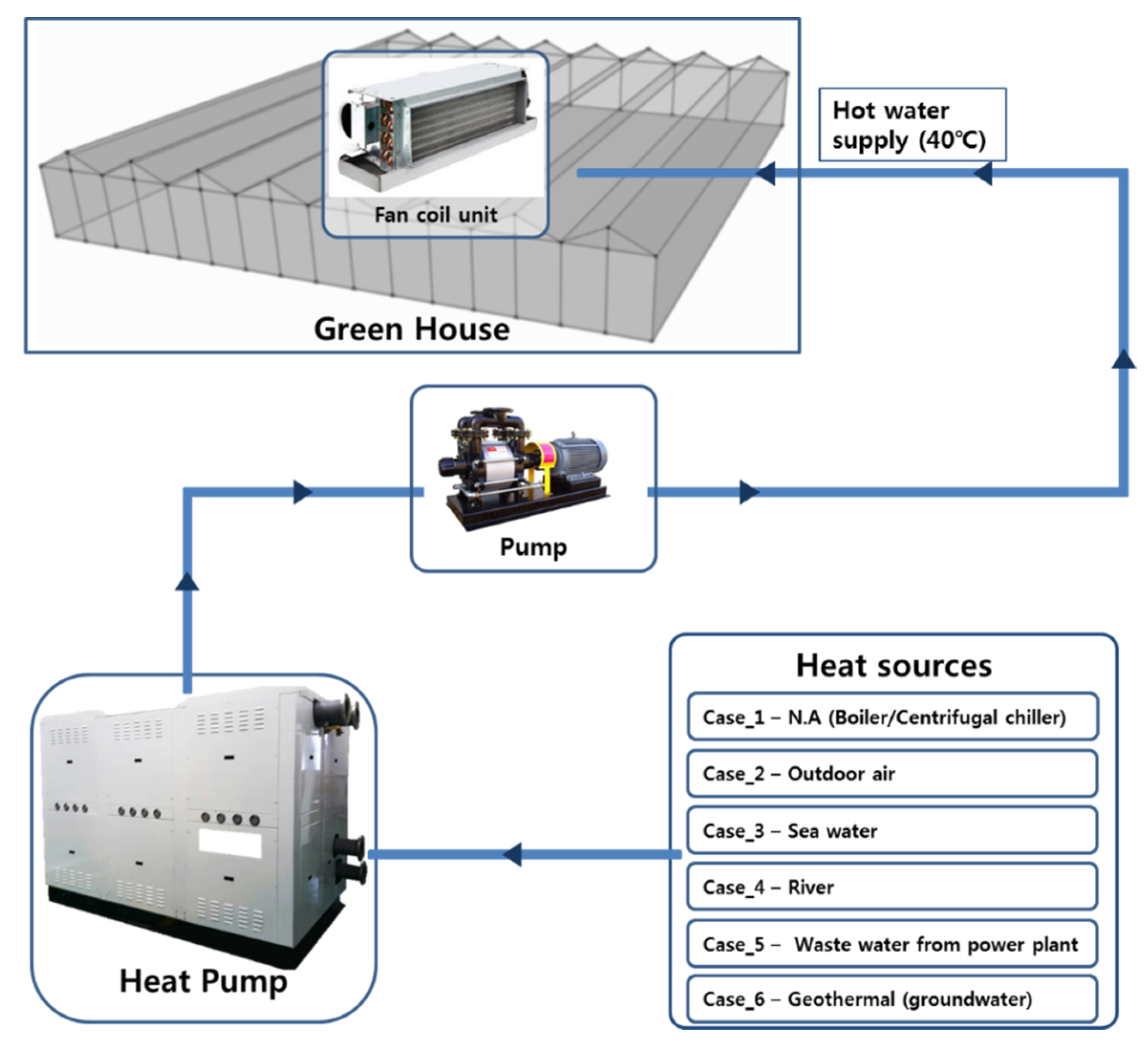
3. Selection of the Pipe Network Parameters

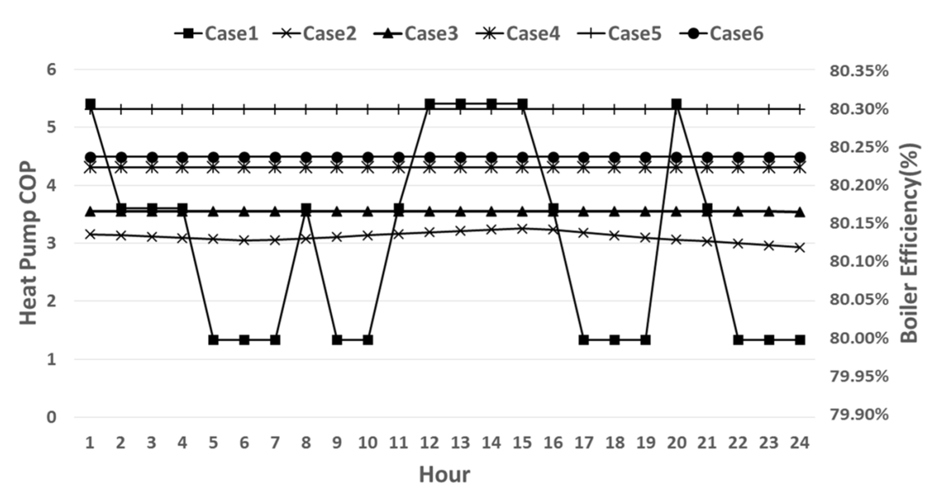
The base model of this study is the same as in the previous study, so it is necessary to arrange the overall patterns including boiler efficiency, performance coefficient of heat pump for each heat source and energy consumption. Also, the load required for this simulation modeling is 1100 kW [6]. Therefore, it is assumed that ten 30RT heat pumps are used. Figure 3 is the graph showing the boiler efficiency and COP of heat pump for each heat source. Case 1 is the base model, and since most of large scale horticulture facilities in the country use gas boilers, the boiler efficiency is used. For the remaining five cases, COP which is the performance coefficient of heat pump which applies the heat source (outdoor air, sea water, river water, power plant waste heat and geothermal heat) is used. Case 1 which is the base model shows approximately 0.4% plus or minus but the efficiency is maintained at 80% around the clock. In cases 2–6 using the heat pump, the average outlet temperature of each heat source including outdoor air, sea water, river water, power plant waste heat and geothermal heat on the representative day is −6.35 °C, 6.49 °C, 10 °C, 20 °C and 11.91 °C respectively and COP which is the performance coefficient is 3.1, 4.0, 4.3, 5.3 and 4.5, respectively. Also, in case of energy consumption, the heat pump using the power plant waste heat which has the highest COP shows the lowest energy consumption for cases 2–6, and the heat pump using the outdoor air which has the lowest COP shows the highest energy consumption. The electricity consumption of heat pump for each heat source is reduced by approximately 75%–85% in comparison to the gas consumption of boiler, so the heat pump is more effective than the boiler in terms of energy savings and economy.

Figure 3. Boiler efficiency and heat pump COP variations [6].

Figure 3. Boiler efficiency and heat pump COP variations [6].

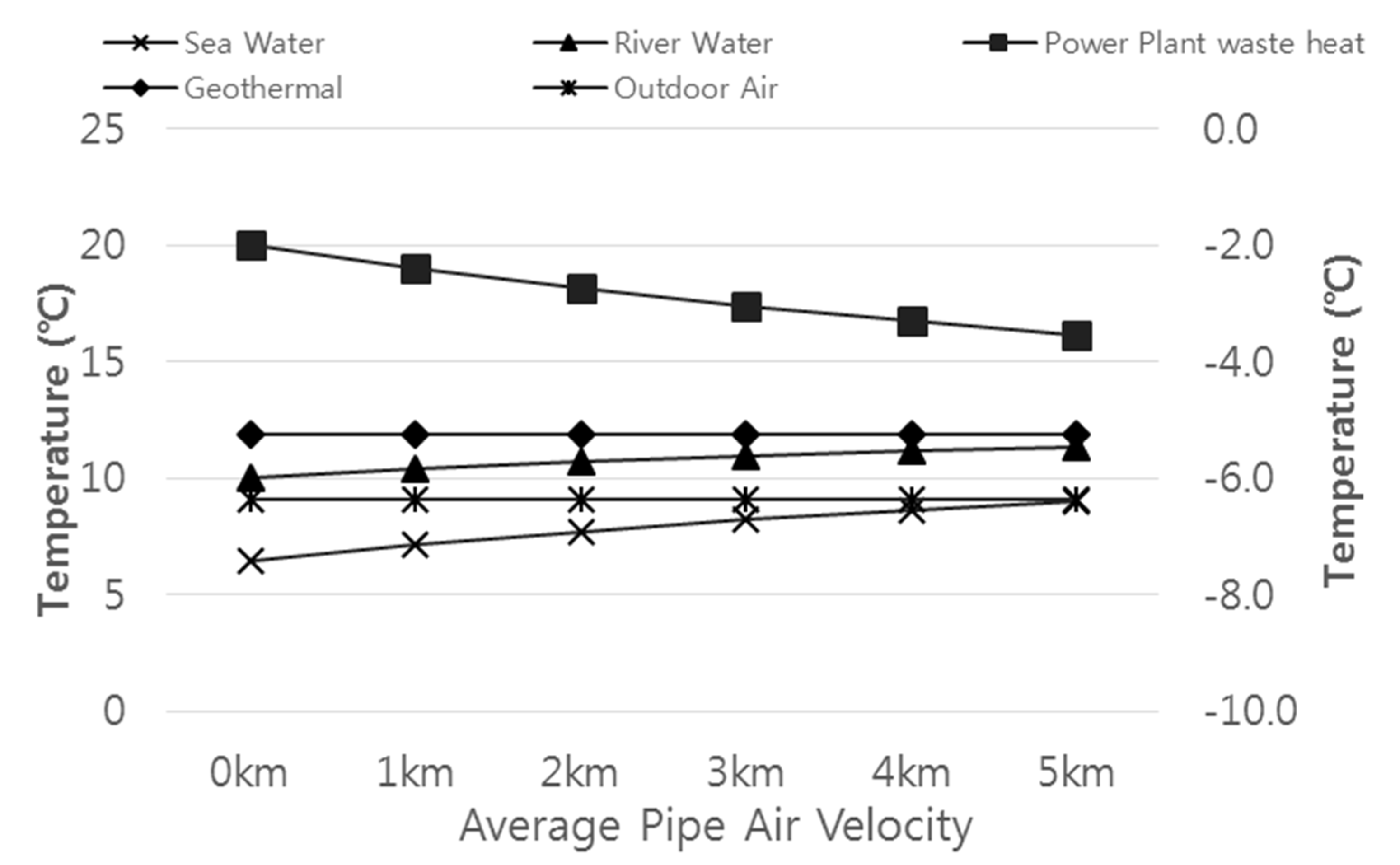
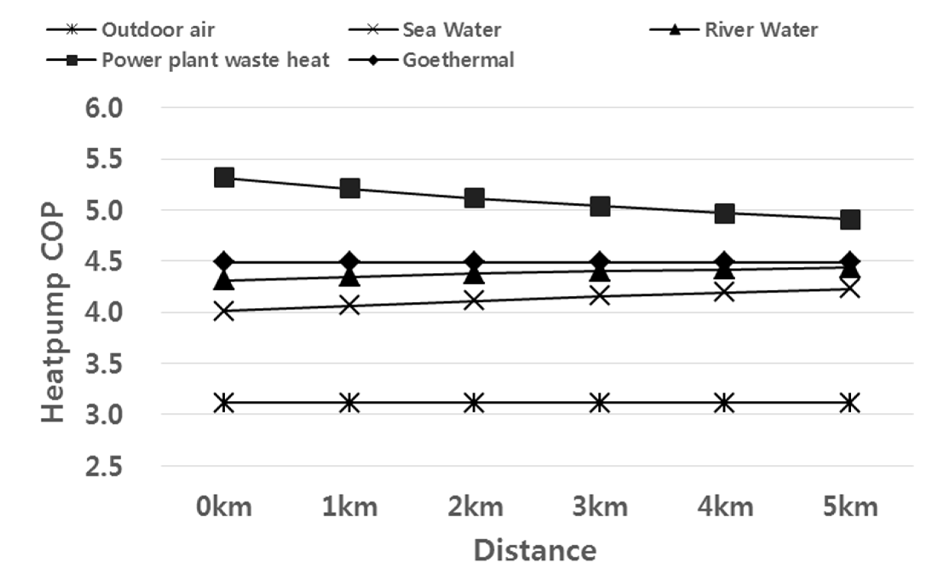
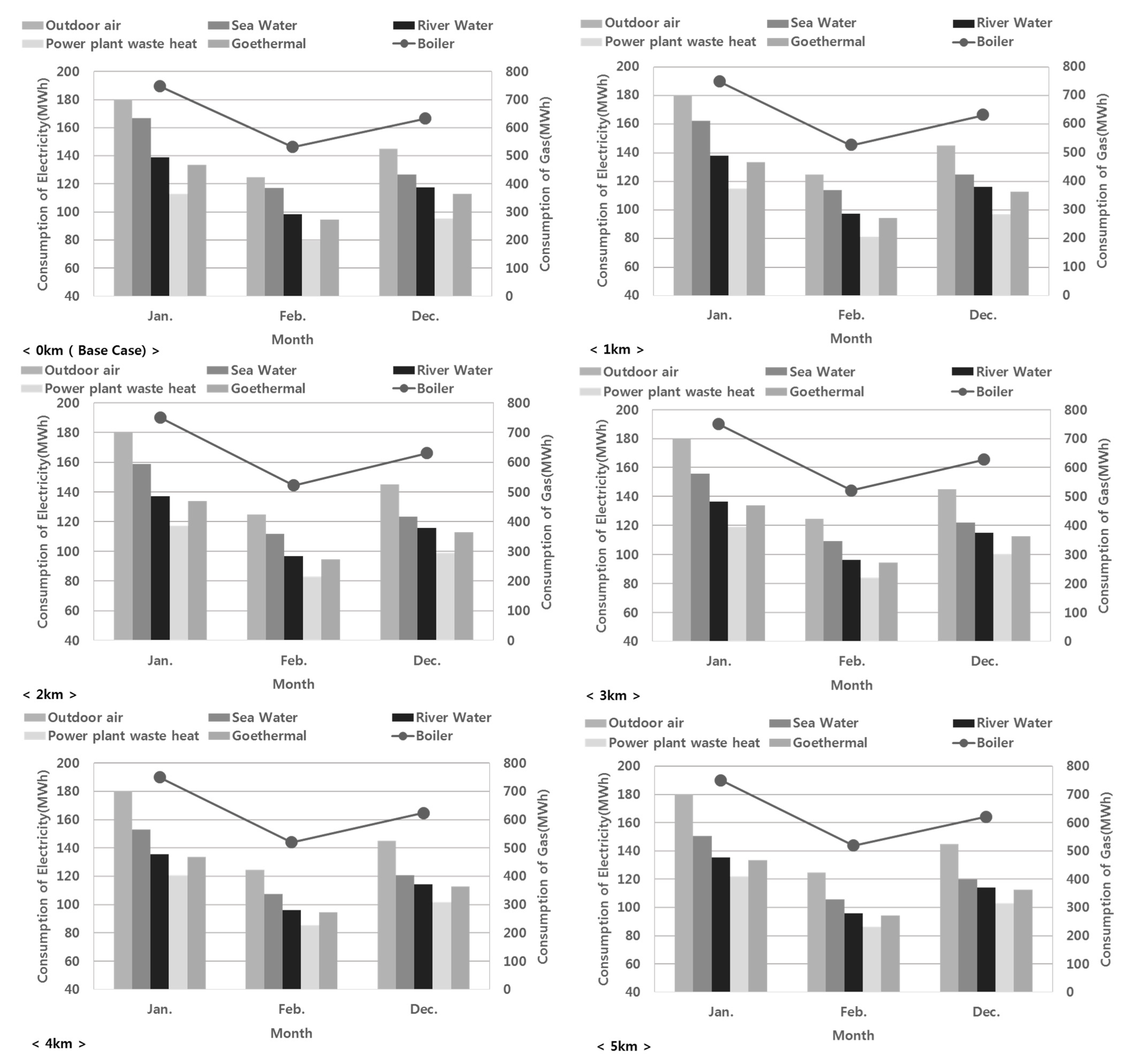
With regards to the study mentioned above, Lee et al. [7] conducted an additional study with the distance from the origin of heat source and the place of use of the heat pump and the material of the pipe used for delivering the heat source as variables and confirmed the outlet temperature, COP of the heat pump and the energy use pattern. For the outlet temperature pattern according to the distance and material, the temperature difference in case of sea water and river water when the material is HDPE is 3.67 °C and 1.29 °C, respectively, as the distance increases from 0 km to 5 km. Also, the temperature difference in the case of sea water and river water for PB and PVC showed a temperature increase of 2.94 °C, 1.04 °C, 2.27 °C and 0.80 °C, respectively, from the heat source origin for a distance of 5 km. On the other hand, in the case of the heat pump using the power plant waste heat as the heat source, the temperature difference was HDPE was 14.53 °C based on the distance of 5 km which showed a larger reduction than 15.62 °C for PB and 16.62 °C for PVC, and the amount of heat loss became larger as the heat conductivity increased. Also, COP of outdoor air, sea water, river water, power plant waste heat and geothermal heat when the distance was 0 km was 3.1, 4.0, 4.3, 5.3 and 4.5, respectively. However, COP in the case of using HDPE material was 3.1, 4.3, 4.4, 4.7 and 4.5, respectively, on average based on the distance of 5 km. In the case when the material was PB, the average COP on the representative day based on the distance of 5 km was 3.1, 4.6, 4.4, 4.8 and 4.5, respectively, and in the case the material was PVC, the average COP on the representative day based on the distance of 5 km was 3.1, 4.2, 4.4, 5.0 and 4.5, respectively. It shows the same form with the temperature pattern for each heat source changing according to the distance. Lastly, for the electricity consumption on the representative day according to the distance and material, the electricity consumption of the heat pump using sea water and river water decreased on average by 5.21% and 1.88%, respectively, as the distance increased from 0 to 5 km when the material was HDPE, and the electricity consumption of the heat pump using the power plant waste heat increased by 8.3%. Also, in the case where the material was PB, the electricity consumption of the heat pump using sea water and river water decreased by 4.38% and 1.57%, respectively, while the electricity consumption of the heat pump using the power plant waste heat increased by 6.93%, and in the case the material was PVC, the electricity consumption of the heat pump using sea water and river water decreased by 3.49% and 1.25%, respectively, while the electricity consumption of the heat pump using the power plant waste heat increased by 5.45%. Therefore, using the heat pump with unused energies for the heating in the horticulture facility provided more energy saving effects than using a gas boiler.

Lee et al. [20] also carried out an additional study by setting the diameter of an underground pipe for delivering the heat source from the origin to the place of use of the heat pump and the flow rate from the precedent study as the variables and fixing the distance at 5 km. The outlet temperature pattern, COP of the heat pump and the energy consumption in case of applying variables to each heat source as same as the study above were compared. In the study of Lee et al. [20], the average outlet temperature of outdoor air and geothermal heat on the representative day according to the pipe diameter was constant regardless of the pipe diameter, and the average outlet temperature of sea water and river water increased slightly when the diameter of pipe was from 25 A to 65 A but decreased when 75 A was set as the pipe diameter. On the other hand, the power plant waste heat showed a pattern where the temperature decreased slightly when the pipe diameter was from 25 A to 65 A but increased when 75 A was set for the pipe diameter. COP and electricity consumption also showed the same pattern with the outlet temperature and the difference in the value was insignificant, so it was concluded that as a variable the pipe diameter had a lesser effect than other variables. The average outlet temperature of sea water and river water according to flow rate inside the pipe also shows a pattern whereby the outlet temperature decreases as the flow rate increases. On the other hand, the power plant waste heat which has a higher temperature than the geothermal heat shows the pattern that the outlet temperature increases as the flow increases. It is considered that it is influenced by changes in the temperature of fluid at the time of reaching the heat pump and COP analyzed above. Therefore, as flow rate increases, the heat gain and heat loss on the outlet temperature for each heat source are reduced, and as the outlet temperature decreases, COP and electricity consumption show the same pattern, and it is considered that the heat pump performance is affected by the outlet temperature of the pipe applied to the heat pump. The overall interpretation will be described in details in this study later. The outlet discharge temperature, COP amount and energy consumption according to variables including the distance, material, diameter and flow rate of pipe for the distance of 5 km from the origin of heat source to the place of use of the heat pump were confirmed. As a result, it was confirmed that the variable which showed the largest difference was distance. Remaining variables including the material, diameter and flow rate of pipe showed lesser differences than the distance, and the pipe diameter showed the most significant difference. Therefore, it is intended to analyze the economic feasibility according to changes in the distance when the conditions including the material, diameter and flow rate of pipe are same. First, HDPE was applied for the material based on the previous study [7] as mentioned above, and 65 A, showing a change of energy consumption pattern, was selected for the diameter of pipe based on the overall electricity consumption pattern and 9.67 kg/s which was the median value of cases mentioned above for the flow rate. Therefore, the analysis of economic feasibility was carried out changing the distance as the factor with the highest influence. Therefore, the analysis was carried out by setting the distance from 0 km to 5 km at 1 km intervals.

4. Energy and CO₂ Emission Analysis

4.1. Average Outlet Temperature on the Representative Day According to the Distance

Table 5 and Figure 4 show average outlet temperature on the representative day of each heat source according to distance [7]. As the distance increased from 0 km to 5 km, the temperature for the cases using outdoor air and geothermal heat was constant, and the temperature for the cases using sea water, river water and power plant waste heat changed. At first, in the case of outdoor air and geothermal heat, it is assumed that the origin of heat source is located always at a close range from the place of use of the heat pump, so the outlet temperature is constant since it is not affected by the distance. In case of sea water and river water, the temperature increases as the distance from the origin of the heat source increases to 5 km. In case of power plant waste heat, the temperature also deceases as the distance increases. This pattern is shown because the heat source moves from the origin to the place of use of the heat pump through the underground pipe, and while moving, the heat source exchanges heat with the geothermal heat temperature, creating a change in the temperature pattern. In case of sea water and river water having the lower temperature pattern than the geothermal heat, the heat source gains heat through the heat exchange with the geothermal heat while moving so that eventually the outlet temperature increases, and in case of power plant waste heat having the higher temperature pattern than the geothermal heat, the heat source loses heat to the geothermal heat while moving so that eventually the outlet temperature decreases [7].

Table 5. Average outlet temperature on the representative day of each heat source according to distance [7].

Distance	Outdoor Air	Sea Water	River Water	Power Plant Waste Heat	Geothermal
0 km	−6.3	6.5	10.0	20.0	11.9
1 km	−6.3	7.1	10.4	19.0	11.9
2 km	−6.3	7.7	10.7	18.2	11.9
3 km	−6.3	8.2	11.0	17.4	11.9
4 km	−6.3	8.7	11.2	16.8	11.9
5 km	−6.3	9.1	11.3	16.2	11.9

Table 5. Average outlet temperature on the representative day of each heat source according to distance [7].

Distance	Outdoor Air	Sea Water	River Water	Power Plant Waste Heat	Geothermal
0 km	−6.3	6.5	10.0	20.0	11.9
1 km	−6.3	7.1	10.4	19.0	11.9
2 km	−6.3	7.7	10.7	18.2	11.9
3 km	−6.3	8.2	11.0	17.4	11.9
4 km	−6.3	8.7	11.2	16.8	11.9
5 km	−6.3	9.1	11.3	16.2	11.9

Figure 4. Average outlet temperature on the representative day of each heat source according to distance [7].

Figure 4. Average outlet temperature on the representative day of each heat source according to distance [7].

4.2. Average COP on the Representative Day of Each Heat Source According to Distance

Table 6 and Figure 5 show average COP on the representative day of each heat source according to distance [7]. The COP calculation form used in this study is that of Hyun et al. [6] which is the base study of this study. Therefore, the same formula was used for COP, and we can see that the factor with the highest influence is the temperature. The formulas regarding COP can be confirmed by the prior study [6]. Like the outlet temperature examined above, the COP pattern of sea water, river water and power plant waste heat, except for outdoor air and geothermal heat changes, as the distance increases from 0 km to 5 km. The heat sources including outdoor air and geothermal heat have no influence according to the distance because it is assumed that the heat sources including outdoor air and geothermal heat are located at a close range from the place of use of the heat pump so that the heat sources are not affected by temperature changes and COP is constant. In the case of heat sources including sea water and river water, COP increases from 4.0 and 4.3 at the distance of 0 km to 4.2 and 4.4 respectively at the distance of 5 km.

Table 6. Average COP on the representative day of each heat source according to distance [7].

Distance	Outdoor Air	Sea Water	River Water	Power Plant Waste Heat	Geothermal
0 km	3.1	4.0	4.3	5.3	4.5
1 km	3.1	4.1	4.3	5.2	4.5
2 km	3.1	4.1	4.4	5.1	4.5
3 km	3.1	4.2	4.4	5.0	4.5
4 km	3.1	4.2	4.4	5.0	4.5
5 km	3.1	4.2	4.4	4.9	4.5

Table 6. Average COP on the representative day of each heat source according to distance [7].

Distance	Outdoor Air	Sea Water	River Water	Power Plant Waste Heat	Geothermal
0 km	3.1	4.0	4.3	5.3	4.5
1 km	3.1	4.1	4.3	5.2	4.5
2 km	3.1	4.1	4.4	5.1	4.5
3 km	3.1	4.2	4.4	5.0	4.5
4 km	3.1	4.2	4.4	5.0	4.5
5 km	3.1	4.2	4.4	4.9	4.5

Figure 5. Average COP on the representative day of each heat source according to distance [7].

Figure 5. Average COP on the representative day of each heat source according to distance [7].

Since COP is highly affected by the temperature, COP increases the same as the temperature pattern studied previously increases as the distance increases. On the other hand, in the case of the power plant waste heat source, COP was 5.3 and 4.9 for the distance of 0 km and 5 km showing that COP decreased as the distance increased, and it was considered that this was same with the temperature pattern. According to COP change, it is mainly affected by the temperature and it is considered that the temperature will have a considerable impact on the calculation of energy consumption in future [7].

4.3. Accumulated Electricity and Gas Consumption on the Winter Season for Each Heat Source According to the Pipe Distance

Figure 6 shows the energy consumption of boiler and heat pump for each heat source during the winter season (December, January, February) [7]. All analysis values from the base case (0 km) to the position of 5 km were lowest on February and highest on January. Low energy consumption was shown on February because the number of days on February was only 28 days, which was smaller than the number of days in January and December and also the outdoor temperature on December or January was higher than the outdoor temperature on February. For the electricity consumption for each heat source, the heat pump using the power plant waste heat which shows the highest COP (performance coefficient of the heat pump) has the lowest electricity consumption, and since the heat pump using the outdoor air shows the lowest COP has the lowest power consumption, so it consumes the largest electrical energy. Also, in case of the heat pump using outdoor air and geothermal heat, it is assumed that heat sources are used at the heat pump position so it is not affected by the distance. Therefore, it shows constant electricity consumption. On the contrary, the electricity consumption of the heat pumps using sea water and river water decreased by 9.90% and 2.74%, respectively, but the electricity consumption of the heat pump using the power plant waste heat increased by 8.28%. This shows the same pattern as the temperature pattern on the representative day of each heat source according to distance studied previously and the electricity consumption of the heat pump for each heat source decreases by approximately 75%–85% in comparison to the gas consumption of the boiler, so it is considered that the heat pump is more advantageous than the boiler in terms of energy savings and economy. The electricity consumption of the heat pump for each heat source is directly affected by COP of each heat source and the energy consumption changes according to the increase or decrease in the outlet temperature according to the distance as a result, so it is considered that these three elements are closely related to each other [7].

Figure 6. Accumulated electricity and gas consumption on the winter season for each heat source according to the pipe distance (W/m²) [7].

Figure 6. Accumulated electricity and gas consumption on the winter season for each heat source according to the pipe distance (W/m²) [7].

4.4. Comparison of Greenhouse Gas Emissions

4.4.1. Summary of CO₂ Emission Calculation

For the greenhouse gas emissions in this study, the emissions of CO₂ which has become the most serious threat to global warming was calculated through the greenhouse gas emission calculation formula presented by the IPCC [21]. In order to calculate the CO₂ emissions according to the emission IPCC calculation formula, ton of oil equivalent (TOE) should be calculated in advance, and it is calculated by using the following Equation (10) [22]:

TOE = Fuel quantity × Net heating value/10⁷ kcal

(10)

TOE is the amount of energy released by burning one ton of crude oil. One TOE represents 10⁷ kcal. The fuel quantity means the total amount of fuel used, and in case of oil conversion factors, IPCC recommends applying the oil conversion factor according to net heating value. Table 7 below shows the net heating value and oil conversion factor of fuel used in this study as the energy calorie conversion standards according to the Framework Act on Energy.

Table 7. Net heating value & oil conversion factor of fuel.

Fuel	Unit	Net Heating Value		Oil Conversion Factor
		Kcal	MJ
LNG	$N{m}^3$	9420	39.4	0.942
Electricity	kWh	2300	9.6	0.23

Table 7. Net heating value & oil conversion factor of fuel.

Fuel	Unit	Net Heating Value		Oil Conversion Factor
		Kcal	MJ
LNG	$N{m}^3$	9420	39.4	0.942
Electricity	kWh	2300	9.6	0.23

Also, ton of carbon (TC) indicates carbon emissions, and it is calculated using Equation (11):

TC = TOE × TC/TOE × Burning ratio

(11)

Here, TC/TOE which is the coefficient of carbon emissions is the carbon intensity and it represents the carbon content of fuel. Also, power is calculated based on CO₂ generated from fuel used for producing electricity, not CO₂ emitted by electricity, so there is no official coefficient of carbon emissions for the power. Therefore, in case of our country, it is recommended to use 0.4585 TCO₂/MWh which is the coefficient of CO₂ emissions developed by Korea Power Exchange in consideration of hydroelectric power generation, nuclear power generation and thermal power generation [23]. In case of LNG gas, the burning ratio is 0.995, and in case of power using bituminous coal as the primary energy, the burning ratio is 0.980. TCO₂ drawn through the process above, which is summarized in Table 8, is as shown in the following Equation (12) [22]:

$$TC{O}_2=TC \times \frac{44({\text{Molecular weight of CO}}_2)}{12(\text{Atomic weight of C})}$$

(12)

Table 8. Coefficient carbon emissions.

Fuel	Coefficient of Carbon Emissions		Coefficient of CO2 Emissions
	Kg C/GC	tonC/Toe	TCO2/MWh
LNG	15.30	0.637	-
Electricity	-	-	0.4585

Table 8. Coefficient carbon emissions.

Fuel	Coefficient of Carbon Emissions		Coefficient of CO2 Emissions
	Kg C/GC	tonC/Toe	TCO2/MWh
LNG	15.30	0.637	-
Electricity	-	-	0.4585

4.4.2. Greenhouse Gas Emissions per Heating Method

Table 9 shows energy usage and CO₂ emissions from the operations during 24 h at the large scale horticulture facility analyzed in the previous study. CO₂ emissions according to the gas consumption drawn through the calculation process presented above were the lowest in February and the highest in January, showing that the CO₂ emissions on January is the highest. Since the number of days in February is smaller than other months and the temperature of the outdoor air on February is higher than the other months, so the consumption of primary energy is reduced and CO₂ emissions also became lower [22].

Table 9. CO₂ emission of gas boiler.

Gas (LNG)	Coefficient of Carbon Emissions (0 km)
	January	February	December
Consumption (MWh)	747.6	530.9	632.8
TOE	64.3	45.7	54.4
TC	40.8	28.9	34.5
TCO2	149.4	106.1	126.5
Total TCO2	382.01

Table 9. CO₂ emission of gas boiler.

Gas (LNG)	Coefficient of Carbon Emissions (0 km)
	January	February	December
Consumption (MWh)	747.6	530.9	632.8
TOE	64.3	45.7	54.4
TC	40.8	28.9	34.5
TCO2	149.4	106.1	126.5
Total TCO2	382.01

Figure 7 shows the CO₂ emissions according to the electricity consumption of a heat pump applying various heat sources. The power plant waste heat showed the lowest emissions, followed by geothermal heat, river water, sea water and outdoor air. In the case of the heat pump using the power plant waste heat, the emission was 132 TCO₂ based on the distance of 0 km and 143 TCO₂ based on the distance of 5 km. The power plant waste heat showed the lowest emissions in comparison to other heat sources, and it is because the temperature distribution of the heat source to be emitted is higher than other heat sources so that the electricity consumption of the compressor is reduced accordingly. In case of comparing TCO₂ emissions between the heat pumps using the power plant waste heat with the lowest TCO₂ emission and the gas boiler used previously, CO₂ emissions are reduced by approximately 63%–65%, so it is considered that it is effective for reducing the emission of greenhouse gases. Also, in case of comparing of greenhouse gas reduction between the heat pump using the outdoor air and the heat pump using the power plant waste heat that showed the largest TCO₂ emissions, the emissions are reduced by approximately 31%–36% even though there is a difference according to the distance, so it is considered that it is also effective. For the pattern of TCO₂ amount for each heat source according to the distance, it is assumed that the heat sources such as outdoor air and geothermal heat are used at a close range from the place of use of the heat pump, so there is no influence according to the distance. In the case of sea water and river water, total TCO₂ deceased as the distance increased, and in case of power plant waste heat, total TCO₂ increased as the distance increased. It shows the same pattern as the temperature pattern analyzed above, so it is considered that the outlet temperature of each heat source has a direct effect in general.

5. LCC Analysis

5.1. Summary of Heating Cost Calculation of Greenhouse Heating System for Each Heat Source

Within the 100 ha horticulture facility modeled for this study, a detailed analysis was performed with 10,000 m² (1 ha) gross area of glass greenhouse for the large-scale horticulture facility and tomato which was one of crops currently cultivated in the controlled agriculture of our country was selected as the greenhouse crop [24].

Figure 7. CO₂ Emission of Heat Pump as a function of pipe network distance from the heat source.

Figure 7. CO₂ Emission of Heat Pump as a function of pipe network distance from the heat source.

For the data of heating cost utilized in the analysis, approximately 3 months from December 1 to February 28 were set as the target period of analysis and the heating energy cost saving rate of heat pump according to each heat source in comparison to gas boiler was calculated. For the rate used in the analysis of heating costs, 20.8447 ₩ (0.02 $)/MJ [25] which was the industrial gas cost during the winter season according to the Seoul City Gas rate standard was applied for gas and the agricultural power rates high voltage (B) of KEPCO was applied for electricity so that 41.9 ₩ (0.04 $)/kWh [26] of energy charge with a basic rate of 1210 KRW was applied. For calculating the gas cost, the rate was applied to the gas consumption at the time of 80% for the heat utilization thermal utilization efficiency of the boiler [24,27]. Also, for the contract power of heat pump for each heat source, it was calculated that 3.5 kW per 1RT of heat pump provided heating to 33.06 m² and 3 which was the average value of the heat pump using the outdoor air was set for COP. As a result, it was analyzed that the capacity of heat pump was 1050 kW when heating 10,000 m² and the contract power at this time was 350 kW. For the application of unit cost to the cost analysis on the initial investment cost, the project expense of 1.3 billion KRW (119,046 $)/ha for agricultural and fisheries energy use efficiency projects (Ministry of Agriculture, Food and Rural Affairs) in 2011 was applied in case of the heat pump using the geothermal heat, and for the application of unit cost of heating pump using other heat sources, the analysis of economic feasibility was carried out based on 1 billion KRW (921,5741 $) per ha of facility cost designed by the Jeju branch of Korea Rural Community Corporation for the 2011 hot and drainage water heat use project [24,27]. Also, in case of pipe laying cost according to increase in the distance, the analysis was carried out based on 386,313,000 KRW per 1 Km extracted from the proved reference. Since there is a difference in the initial cost, it is expected that there will be a difference in the payback period between the geothermal heat and other heat sources.

5.2. Operation Cost Calculation

For the calculation of operation cost for each system, gas and electricity consumptions were calculated first in consideration of cooling and heating loads and COP of each system and the monthly consumption on the winter season was converted to the cost for comparison. The operation cost was calculated by referring to the rate base table of Seoul City Gas and the agricultural power rate calculation standard of KEPCO [24,27].

Figure 8 shows the monthly operation cost of each heat source during the winter season calculated in consideration of distance change from 0 km to 5 km. First of all, the gas cost of a normal boiler in the winter season was approximately 143,448,000 KRW (130,725 $) for 3 months, showing the highest gas cost. In case of the heat pump using outdoor air as the heat source and the heat pump using geothermal heat as the heat source, the gas cost was 20,126,000 KRW (18,345 $) and 15,552,000 KRW (14,175 $) respectively, regardless of the distance. Since it is assumed in the initial setup that the heat source is used at a close range from the place of use of the heat pump for a normal boiler, heat pump using outdoor air as the heat source and the heat pump using geothermal heat as the heat source, the same operation cost is calculated regardless of the distance. On the other hand, the operation cost in case of sea water and river water was 18,468,000 KRW (16,883 $) and 16,113,000 KRW (14,705 $) respectively based on a 0 km distance, and when the distance increased to 5 km, the operation cost was 17,027,000 KRW (15,520 $) and 15,726,000 KRW (14,334 $), respectively. Since the heat sources including sea water and river water have a lower temperature pattern than geothermal heat, the outlet temperature increases as the distance increases, and COP increases and the electricity consumption decreases accordingly so that the operation cost is also reduced. On the contrary, in case of the power plant waste heat having a higher temperature pattern than the geothermal heat, the operation cost was 13,335,000 KRW (12,155 $) based on 0 km and 14,335,000 KRW (13,066 $) based on 5 km, showing that the operation cost increased as the distance increased. It shows the opposite pattern with the analysis using sea water and river water as the heat sources. Therefore, it shows the same pattern with the outlet temperature of each heat source as the distance increases, and COP, electricity consumption and operation cost also show the same pattern accordingly, so it is considered that the operation cost is also closely related to the outlet temperature. In the case of the heat pump using the power plant waste heat which shows the highest efficiency in comparison to the normal gas boiler, the heating energy cost in the winter season is reduced by approximately 70%–90% as the distance increases. Also, the heating energy saving rate of heat pump using the power plant waste heat in comparison to the heat pump using the outdoor air which shows the lowest efficiency among the heat sources is approximately 35%, so it is more effective to use the heat pump for heating than to use a normal gas boiler.

Figure 8. Gas & electric consumption and operation cost according to distance (Unit: $).

Figure 8. Gas & electric consumption and operation cost according to distance (Unit: $).

5.3. Life Cycle Cost Analysis (Payback Period)

Table 10 shows the payback period in comparison to the initial investment cost of the heat pump for each heat source analyzed through LCC analysis in comparison to the gas boiler. Installing the heat pump for each heat source at a large scale horticulture facility requires a large initial cost in comparison to the previous gas heating, and as the distance increases, additional construction costs will be incurred for pipe laying, further increasing the initial cost. However, the operation cost for using energy could be reduced, so in the case of the heat pumps using outdoor air and geothermal heat, the payback period was 8.11 years and 10.17 years, respectively, regardless of the distance. This is why a short distance is set for the distance the same as the outlet temperature, COP and electricity consumption analyzed previously. In the case of heat pumps using sea water and river water, the recovery period was 8.00 years and 7.86 years, respectively, based on the distance of 0 km and 23.19 years and 22.97 years based on the distance of 5 km. As the distance increases, the operation cost is reduced so that the amount of energy saved increases but the payback period increases, and this is because, as the distance increases, the initial investment amount increases due to the additional pipe installation costs and the payback period increases accordingly. Also, in the case of the heat pump using the power plant waste heat, the payback period was 7.69 years based on the distance of 0 km and 22.71 years based on the distance of 5 km. Therefore, it is determined that the heat pump using the power plant waste heat as the heat source is the most effective in the case of a short distance between the origin of the heat source and the place of use of the heat pump, and based on 5 km, the heat pump using the geothermal heat as the heat source is the most effective as the distance increases. Also, it is considered that the energy saving rate of heat pump using the power plant waste heat is higher than the heat pump using the geothermal heat in case the payback period is exceeded, so the heat pump using the power plant waste heat is also effective.

Table 10. Cost benefit analysis according to distance (Won, $/ha).

Distance	Description	Outdoor Air	Sea Water	River Water	Power Plant Waste Heat	Geothermal
0 km	Equipment cost	1,000,000 (921,574 $)	1,000,000 (921,574 $)	1,000,000 (921,574 $)	1,000,000 (921,574 $)	1,300,000 (119,046 $)
	Annual reduction in energy expenses	123,293 (113,623 $)	124,951 (115,152 $)	127,286 (117,001 $)	130,084 (119,573 $)	127,867 (117,839 $)
	Payback period	8.11	8.00	7.86	7.69	10.17
1 km	Equipment cost	1,000,000 (921,574 $)	1,386,313 (1,277,590 $)	1,386,313 (1,277,590 $)	1,386,313 (1,277,590 $)	1,300,000 (119,046 $)
	Annual reduction in energy expenses	123,293 (113,623 $)	125,327 (115,498 $)	127,411 (117,418 $)	129,838 (119,655 $)	127,867 (117,839 $)
	Payback period	8.11	11.06	10.88	10.68	10.17
2 km	Equipment cost	1,000,000 (921,574 $)	1,772,626 (1,633,606 $)	1,772,626 (1,633,606 $)	1,772,626 (1,633,606 $)	1,300,000 (119,046 $)
	Annual reduction in energy expenses	123,293 (113,623 $)	125,653 (115,798 $)	127,509 (117,509 $)	129,617 (119,452 $)	127,867 (117,839 $)
	Payback period	8.11	14.11	13.90	13.68	10.17
3 km	Equipment cost	1,000,000 (921,574 $)	2,158,939 (1,989,622 $)	2,158,939 (1,989,622 $)	2,158,939 (1,989,622 $)	1,300,000 (119,046 $)
	Annual reduction in energy expenses	123,293 (113,623 $)	125,935 (115,760 $)	127,585 (117,277 $)	129,419 (118,962 $)	127,867 (117,839 $)
	Payback period	8.11	17.14	16.92	16.68	10.17
4 km	Equipment cost	1,000,000 (921,574 $)	2,545,252 (2,345,638 $)	2,545,252 (2,345,638 $)	2,545,252 (2,345,638 $)	1,300,000 (119,046 $)
	Annual reduction in energy expenses	123,293 (113,623 $)	126,180 (115,985 $)	127,286 (117,286 $)	129,242 (118,809 $)	127,867 (117,839 $)
	Payback period	8.11	20.17	20.00	19.69	10.17
5 km	Equipment cost	1,000,000 (921,574 $)	2,931,565 (2,701,654 $)	2,931,565 (2,701,654 $)	2,931,565 (2,701,654 $)	1,300,000 (119,046 $)
	Annual reduction in energy expenses	123,293 (113,623 $)	126,392 (116,180 $)	127,645 (117,332 $)	129,084 (118,655 $)	127,867 (117,839 $)
	Payback period	8.11	23.19	22.97	22.71	10.17

Table 10. Cost benefit analysis according to distance (Won, $/ha).

Distance	Description	Outdoor Air	Sea Water	River Water	Power Plant Waste Heat	Geothermal
0 km	Equipment cost	1,000,000 (921,574 $)	1,000,000 (921,574 $)	1,000,000 (921,574 $)	1,000,000 (921,574 $)	1,300,000 (119,046 $)
	Annual reduction in energy expenses	123,293 (113,623 $)	124,951 (115,152 $)	127,286 (117,001 $)	130,084 (119,573 $)	127,867 (117,839 $)
	Payback period	8.11	8.00	7.86	7.69	10.17
1 km	Equipment cost	1,000,000 (921,574 $)	1,386,313 (1,277,590 $)	1,386,313 (1,277,590 $)	1,386,313 (1,277,590 $)	1,300,000 (119,046 $)
	Annual reduction in energy expenses	123,293 (113,623 $)	125,327 (115,498 $)	127,411 (117,418 $)	129,838 (119,655 $)	127,867 (117,839 $)
	Payback period	8.11	11.06	10.88	10.68	10.17
2 km	Equipment cost	1,000,000 (921,574 $)	1,772,626 (1,633,606 $)	1,772,626 (1,633,606 $)	1,772,626 (1,633,606 $)	1,300,000 (119,046 $)
	Annual reduction in energy expenses	123,293 (113,623 $)	125,653 (115,798 $)	127,509 (117,509 $)	129,617 (119,452 $)	127,867 (117,839 $)
	Payback period	8.11	14.11	13.90	13.68	10.17
3 km	Equipment cost	1,000,000 (921,574 $)	2,158,939 (1,989,622 $)	2,158,939 (1,989,622 $)	2,158,939 (1,989,622 $)	1,300,000 (119,046 $)
	Annual reduction in energy expenses	123,293 (113,623 $)	125,935 (115,760 $)	127,585 (117,277 $)	129,419 (118,962 $)	127,867 (117,839 $)
	Payback period	8.11	17.14	16.92	16.68	10.17
4 km	Equipment cost	1,000,000 (921,574 $)	2,545,252 (2,345,638 $)	2,545,252 (2,345,638 $)	2,545,252 (2,345,638 $)	1,300,000 (119,046 $)
	Annual reduction in energy expenses	123,293 (113,623 $)	126,180 (115,985 $)	127,286 (117,286 $)	129,242 (118,809 $)	127,867 (117,839 $)
	Payback period	8.11	20.17	20.00	19.69	10.17
5 km	Equipment cost	1,000,000 (921,574 $)	2,931,565 (2,701,654 $)	2,931,565 (2,701,654 $)	2,931,565 (2,701,654 $)	1,300,000 (119,046 $)
	Annual reduction in energy expenses	123,293 (113,623 $)	126,392 (116,180 $)	127,645 (117,332 $)	129,084 (118,655 $)	127,867 (117,839 $)
	Payback period	8.11	23.19	22.97	22.71	10.17

Figure 9. Payback period according to distance (Year).

Figure 9. Payback period according to distance (Year).

6. Conclusions

In this study, the modeling of a glass greenhouse for a large-scale horticulture facility was carried out with EnergyPlus, and the electricity/gas consumption were compared and analyzed with the diameter of pipe, flow rate, distance and material of pipe as variables in the process to deliver the heat source from its origin to the place of use of the heat pump. Also, an analysis of economic feasibility comparing the electricity bill according to the electricity consumption of the heat pump for each heat source in comparison to the gas cost according to the gas consumption of a normal gas boiler was carried out. The conclusions of this study are as follows:

• It was confirmed through the comparison with the precedent studies that the outlet temperature, COP and electricity consumption according to the analysis conditions of this study showed the same pattern. The heat pump using the power plant waste heat showed the lowest CO₂ emissions, followed by geothermal heat, river water, sea water and outdoor air. In the case of the heat pump using power plant waste heat, the emissions were 132 TCO₂ based on the distance of 0 km and as the distance increased, based on the distance of 5 km. In case comparing TCO₂ emissions between the heat pumps using the power plant waste heat with the lowest TCO₂ emission and the gas boiler used previously, CO₂ emissions are reduced by approximately 63%–65%, so it is considered that it is effective for reducing the greenhouse gas emissions. The pattern of TCO₂ for each heat source according to the distance is same as the temperature pattern analyzed above, so it is considered that it is closely related with the outlet temperature of each heat source in general.
• According to the analysis conditions of this study, the operation cost of heat pump using outdoor air as the heat source was 20,126,300 KRW (18,315$) based on the winter season and the operation cost of heat pump using geothermal heat as the heat source was 15,551,920 KRW (14,152 $). The outdoor air and geothermal heat are not affected by the distance so that the same operation cost is shown regardless of the distance. The operation cost of the heat pumps using sea water and river water as the heat source were 18,467,550 KRW (16,805 $) and 16,113,340 KRW (14,663 $), respectively, based on 0 km and 17,026,730 KRW (15,494 $) and 15,726,340 KRW (14,311 $) based on 5 km, showing that the operation cost decreased as the distance increased. On the other hand, the operation cost of the heat pump using the power plant waste heat was 13,335,370 KRW (12,135 $) based on 0 km and 14,334,660 KRW (13,045 $) based on 5 km, showing that the operation cost increased as the distance increased. In the case of the operation cost, it is calculated based on the electricity consumption which is significantly affected by the outlet temperature and COP, and increase or decrease in the operation cost for each heat source as the distance increases shows the same pattern as the outlet temperature according to the distance.
• The payback period of the heat pump using the outdoor air and sea water as the heat source in comparison to the initial investment cost calculated through LCC analysis was 8.11 years and 10.17 years, respectively, regardless of the distance. The payback periods of the heat pumps using sea water, river water and power plant waste heat as the heat source were 8.00 years, 7.86 years and 7.69 years, respectively, based on 0 km and 23.19 years, 22.97 years and 22.71 years, respectively, based on 5 km. This is because the investment cost including the pipe installation cost increased as the distance increased so that the payback period became longer. Based on the distance of 0 km, it is considered that using the power plant waste heat which has the highest temperature of heat source is the most effective, and in the case of geothermal heat, the payback period became longer than that of other heat sources due to the difference in the initial investment cost. However, it is considered that the heat pump using the geothermal heat is more effective as the distance increases, and since the heat pump using the power plant waste heat has the highest operation cost payback amount, so it is considered that based on the distance of 5 km, the heat pump using the power plant waste heat would be also effective only if the payback period is surpassed.

References

1. Yang, C.H. Economical Analysis of a Small Capacity Water Source Heat Pump Utilizing Unused Energy of Underground Water Tank. Ph.D. Dissertation, Seoul National University of Science and Technology, Seoul, Korea, 2012. [Google Scholar]
2. Park, B.H.; Jung, G.J.; Im, Y.B. LCC comparison of ground source energy with fossil fuel energy through renewal case of building mechanic equipment. In Proceedings of the Fall Conference of Architectural Institute of Korea (AIK), Seoul, Korea, July 2007; pp. 858–865.
3. Yun, C.H.; Kang, B.H.; Kim, S.H. Greenhouse gas reduction analysis of district cooling using waste heat from CHP systems. In Proceedings of the Summer Conference of In Proceedings of the Winter Conference of the Society of Air-Conditioning and Refrigerating Engineers of Korea (SAREK), Yongpyong, Korea, June 2010; pp. 655–660.
4. Heo, T. On the Application of the Heat Pump System to Facility Horticulture, Using Hot Waste Water from Power Plants. Ph.D. Dissertation, Jeju National University, Jeju, Korea, 2012. [Google Scholar]
5. Jung, G.J. Green House Gases comparison of GSHP with EHP and GHP based on conversion data of annual electric energy consumption of GSHP in child care building. J. AIK 2008, 32, 337–343. [Google Scholar]
6. Hyun, I.T.; Lee, J.H.; Yoon, Y.B.; Lee, K.H.; Nam, Y.J. The potential and utilization of unused energy source for large-scale horticulture facility applications under Korean climatic conditions. Energies 2014, 7, 4781–4801. [Google Scholar] [CrossRef]
7. Lee, J.H.; Yoon, Y.B.; Hyun, I.T.; Lee, K.H. Effect of pip network materials and distance on unused energy source system performance for large-scale horticulture facilities. J. Korea Instit. Ecol. Archit. Environ. (KIEAE) 2014, 14, 119–125. [Google Scholar]
8. EnergyPlus. Testing and Validation. Available online: http://apps1.eere.energy.gov/buildings/energyplus/testing.cfm (accessed on 28 February 2015).
9. Kim, Y.H. A Study of Geothermal Heat Pump Performance Prediction and Assessment Technique. Ph.D. Dissertation, Jeju National University, Jeju, Korea, 2007. [Google Scholar]
10. Choi, S.W. A Study on Thermal Conductivity Characteristics of Deep Depth Vertical Closed-Loop Ground Heat Exchanger. Master Thesis, Kwangwoon University, Seoul, Korea, 2012. [Google Scholar]
11. Guidance on Energy Efficient Farm Product Management in Greenhouses; Rural Development Administration (RDA): Suwon, Korea, 2011; pp. 2–3.
12. Crawley, D.B.; Lawrie, L.K.; Winkelmann, F.C.; Buhl, W.F.; Huang, H.J.; Pedersen, C.O.; Strand, R.K.; Liesen, R.J.; Fisher, D.E.; Witte, M.J.; et al. EnergyPlus: Creating a new-generation building energy simulation program. Energy Build. 2001, 33, 319–331. [Google Scholar] [CrossRef]
13. Kim, S.U. Energy simulation technology trend. J. Soc. Air-Cond. Refrig. Eng. Korea (SAREK) 2014, 43, 23–38. [Google Scholar]
14. ASHRAE Fundamentals Handbook; American Society of Heating, Refrigerating and Air-Conditioning Engineers, Inc.: Atlanta, GA, USA, 2009.
15. Fabrizio, E. Energy reduction measures in agricultural greenhouses heating: Envelope, system and solar energy collection. Energy Build. 2012, 53, 57–63. [Google Scholar] [CrossRef]
16. Kim, K.S.; Yoon, J.H.; Song, I.C. Energy performance evaluation of heat reflective radiant barrier systems for greenhouse night insulation. Archit. Inst. Korea (AIK) 2000, 16, 153–161. [Google Scholar]
17. Standard Test Method for Determining Air Leakage Rate by Fan Pressurization. In Active Standard No. ASTM E 779-87; American Society for Testing and Materials (ASTM): West Conshohocken, PA, USA, 1987.
18. Jacovides, C.P.; Mihalakakou, G. An underground pipe system as an energy source for cooling/heating purposes. Renew. Energy 1995, 11, 893–900. [Google Scholar] [CrossRef]
19. Lee, K.H.; Strand, R.K. Implementation of an earth tube system into EnergyPlus program. In Proceedings of the 2nd National Conference of IBPSA-USA (SimBuild 2006), Cambridge, MA, USA, 2–4 August 2006.
20. Lee, J.H.; Yoon, Y.B.; Hyun, I.T. Effects of pipe network diameter and flow rate on unused energy source system performances in large-scale horticulture facilities. In Proceedings of the ASim 2014, IBPSA Asia Conference, Nagoya, Japan, 28–29 November 2014.
21. Kang, H.G. A Study on the Parameter of Ground Source Heat Pump System and Optimal Design Condition. Master Thesis, The University of Seoul, Seoul, Korea, 2012. [Google Scholar]
22. Hyun, I.T.; Lee, J.H.; Yoon, Y.B.; Lee, K.H. CO2 Emission by Heat Pump System using Unused Energy Sources in Large-scale Greenhouse. In Proceedings of the Winter Conference of the Society of Air-Conditioning and Refrigerating Engineers of Korea (SAREK), Seoul, Korea, 2014; pp. 340–343.
23. Korea Power Exchange (KPX). Available online: http://www.kpx.or.kr (accessed on 28 February 2015).
24. Hyun, I.T.; Lee, J.H.; Yoon, Y.B.; Lee, K.H. Economic assessment of employing unused energy sources in large-scale horticulture facilities. In Proceedings of the ASim 2014, IBPSA Asia Conference, Nagoya, Japan, 28–29 November 2014; pp. 238–245.
25. Seoul City Gas. Available online: Http://www.seoulgas.co.kr/front/payment/gasPayTable.do (accessed on 15 July 2014).
26. Korean Electric Power Corporation (KEPCO). Available online: http://cyber.kepco.co.kr/ckepco/front/jsp/CY/E/E/cyeehp00101.jsp (accessed on 15 July 2014).
27. Lee, J.H.; Hyun, I.T.; Yoon, Y.B.; Lee, K.H. LCC Analysis depending on pipe network distance of unused energy source systems in large-scale horticulture facility. In Proceedings of the Winter Conference of the Society of Air-Conditioning and Refrigerating Engineers of Korea (SAREK), Seoul, Korea, 2014; pp. 393–396.