
Wheel Slip Control for Improving Traction-Ability and Energy Efficiency of a Personal Electric Vehicle


Abstract
:1. Introduction
- Quick torque generation by in-wheel driving motors.
- Easy torque measurement from current sensing.
- Left and right independent wheel torque control.
- (1)
- design of a sliding mode wheel slip controller for improving traction performances of commercial electric vehicles equipped with in-wheel-motors;
- (2)
- development of the cost-free vehicle velocity estimator based on the measured motor torques and wheel velocities (which are obtained from the resolvers);
- (3)
- integration of the sliding mode controller and vehicle velocity estimator to actively control the driving wheels for avoiding wheel spin phenomenon;
- (4)
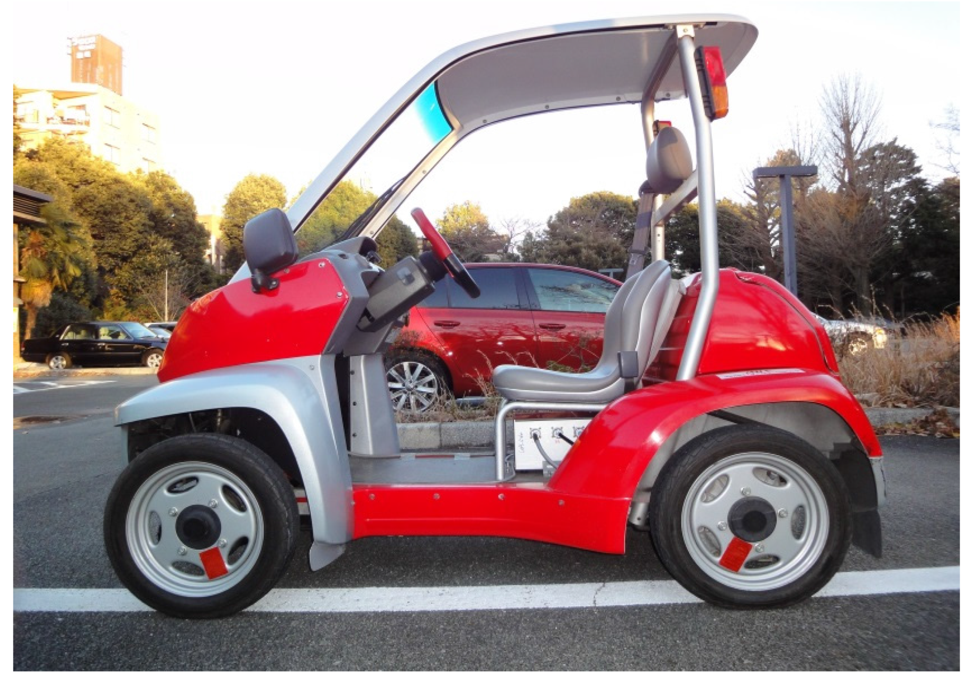
- implementation of the proposed traction control system on a commercial electric vehicle, shown in Figure 1.
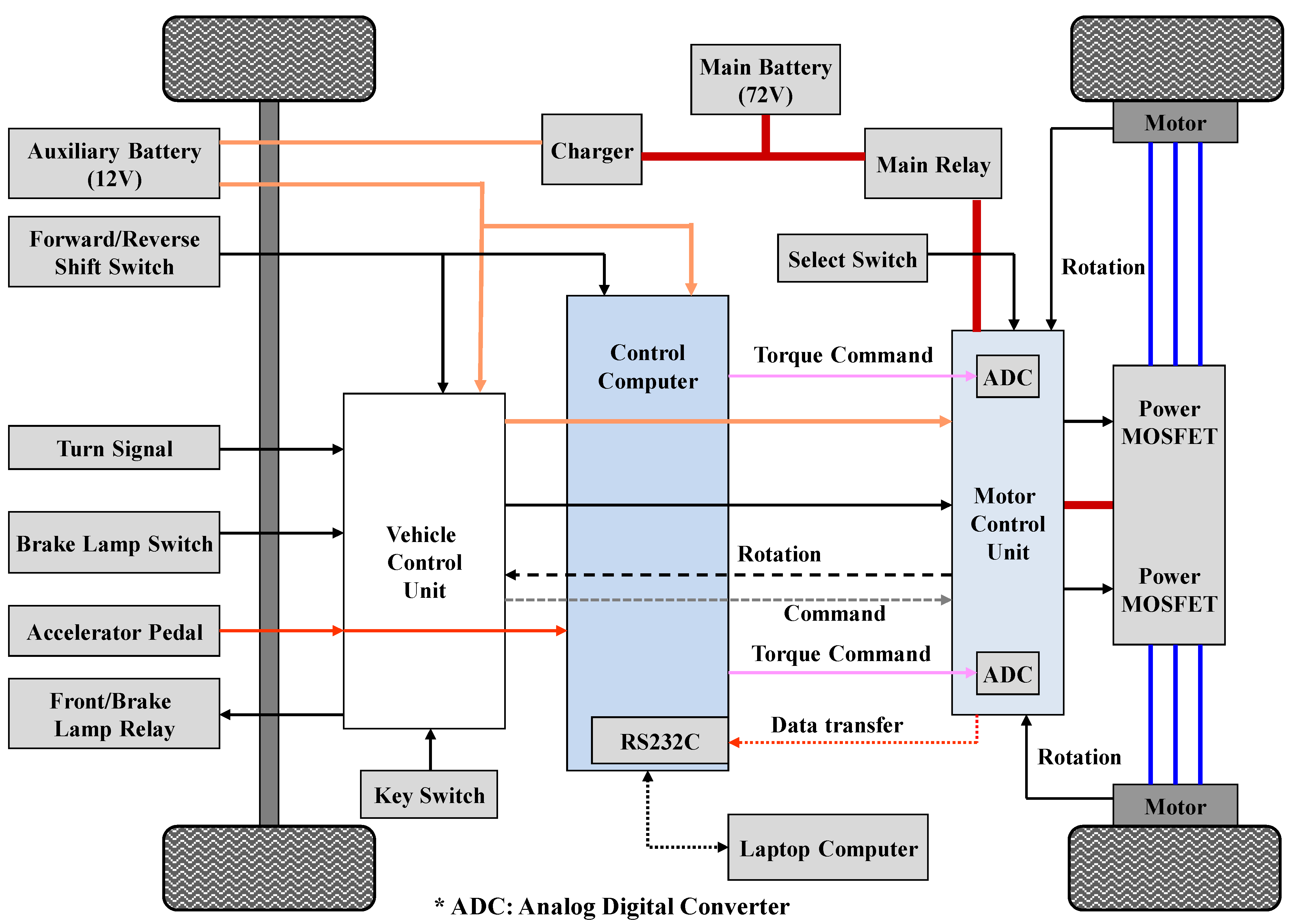
2. Overview of an Experimental Electric Vehicle
- In-wheel motors (i.e., interior permanent magnet synchronous motors) are mounted in the left and right rear wheels, respectively. Thus, each motor can be controlled independently.
- The control computer, which operates the traction control, is used for the realization of the developed control algorithms as well as the sensor signal processing.


| Driving Motor | 2 Permanent Magnet Motors (Rear Wheels) |
|---|---|
| Maximum power | 2 kW × 2 |
| Maximum torque | 100 Nm × 2 |
| Total weight | 360 kg |
| Wheel inertia | 0.5 kg·m² |
| Wheel radius | 0.22 m |
| Sampling time | 0.01 s |
| Controller | PentiumM1.8G, ART-Linux |
| A/D and D/A | 12 bit |
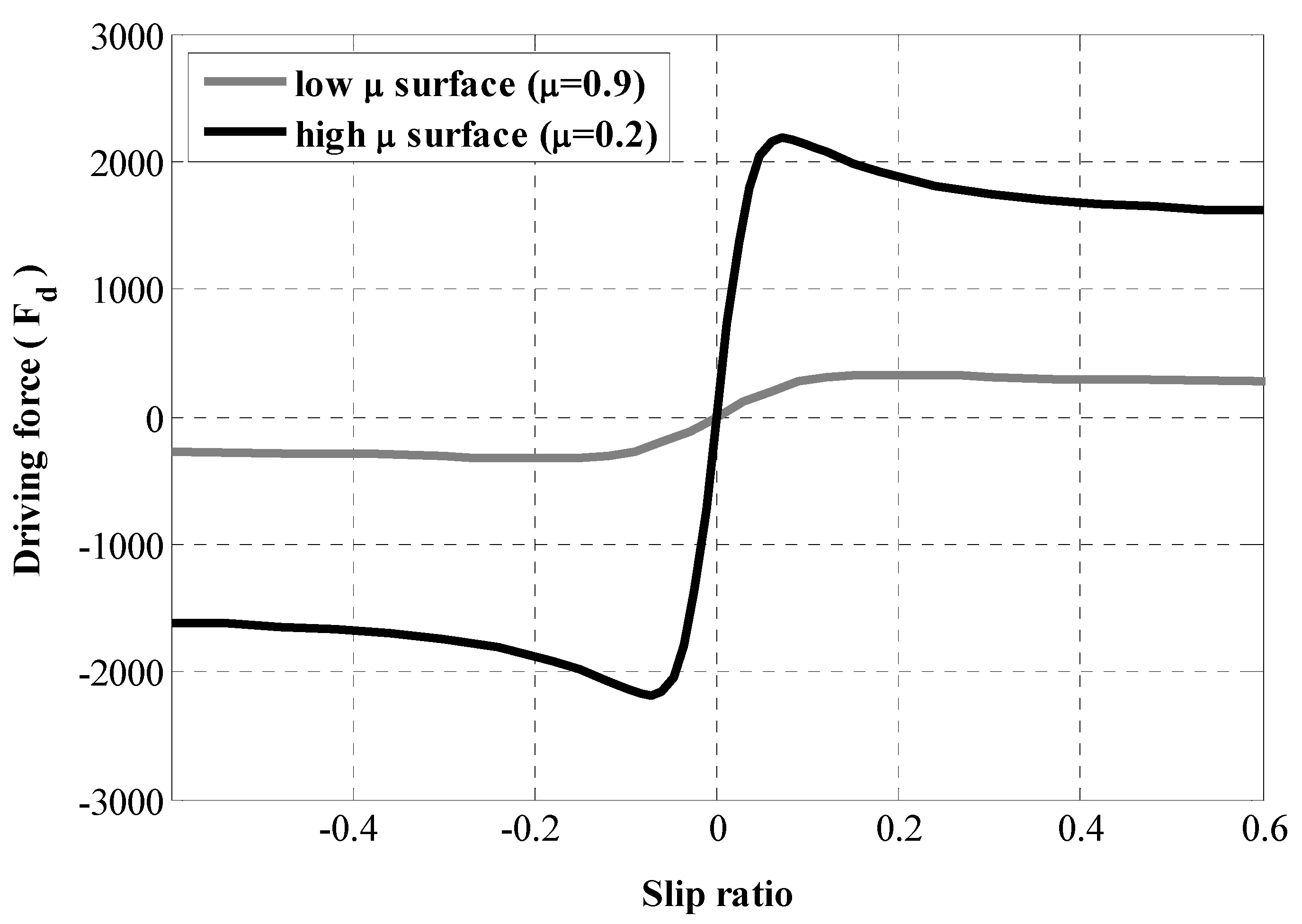
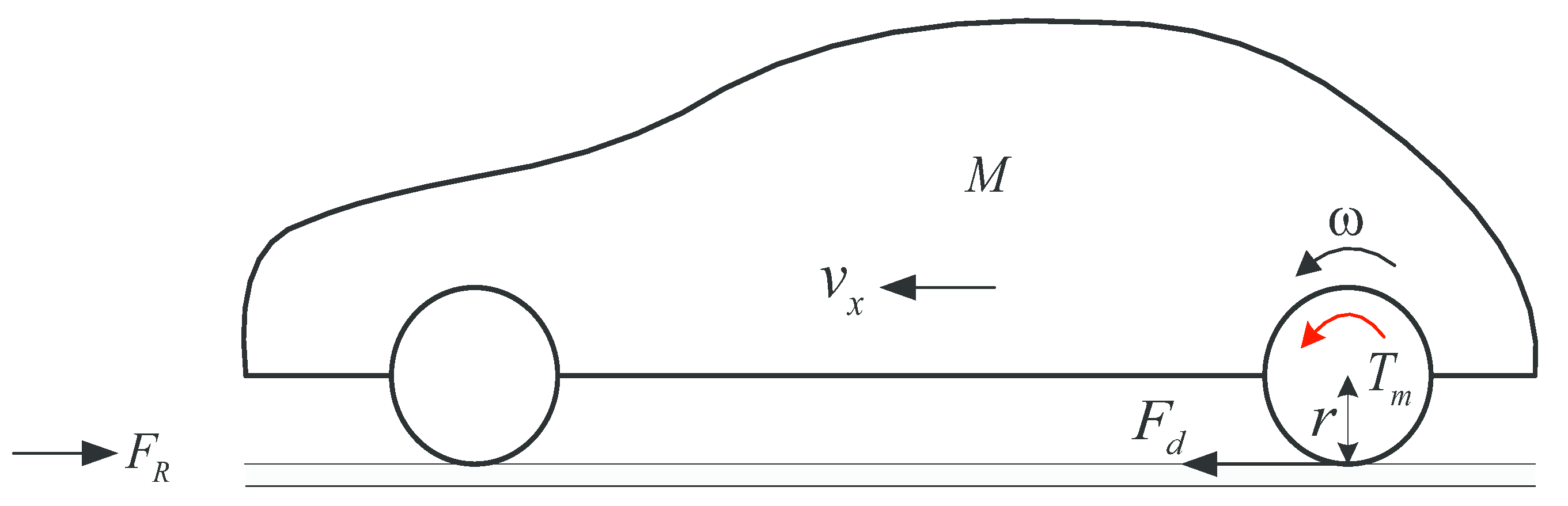
3. Vehicle Model
- Vehicle mass is distributed on each wheel equivalently.
- The lateral, yawing, pitch, and roll dynamics are neglected.

4. Design of a Traction Control System
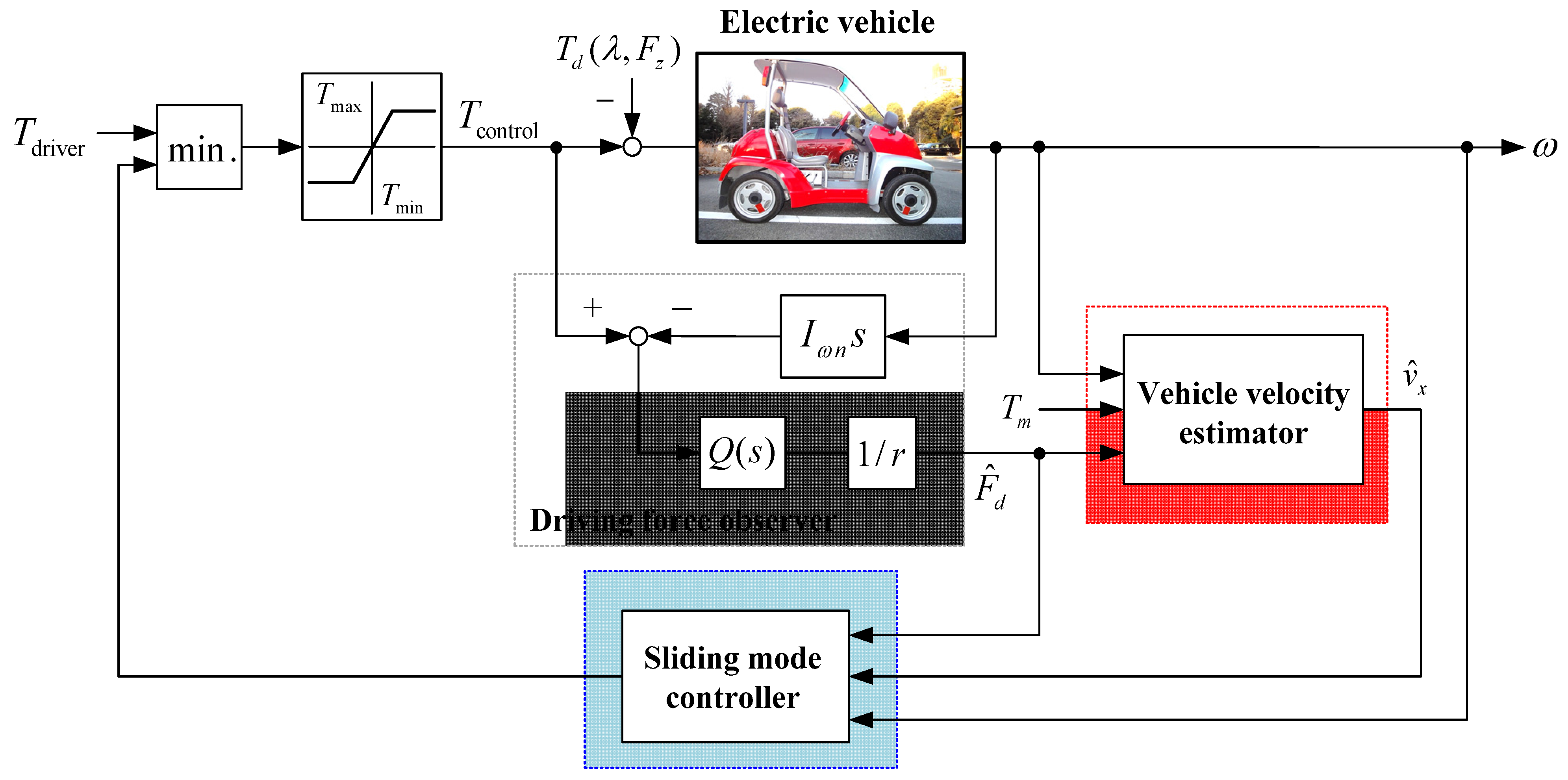
4.1. Overview of a Proposed Control System
- Feedback controller: a sliding mode control approach is applied to achieve robust tracking control of the wheel slip ratio and its asymptotical stability is proven by employing the Lyapunov function.
- Driving force observer: in order to monitor wheel status in real-time, a driving forces observer is designed based on rotational wheel dynamics and measurable motor torque and rotational wheel velocity.
- Vehicle velocity estimator: to realize the control law, generated from a sliding mode controller, real-time information on the vehicle velocity is required. A vehicle velocity estimator using rule-based logic is designed and evaluated by field test results.

4.2. Design of a Sliding Mode Controller
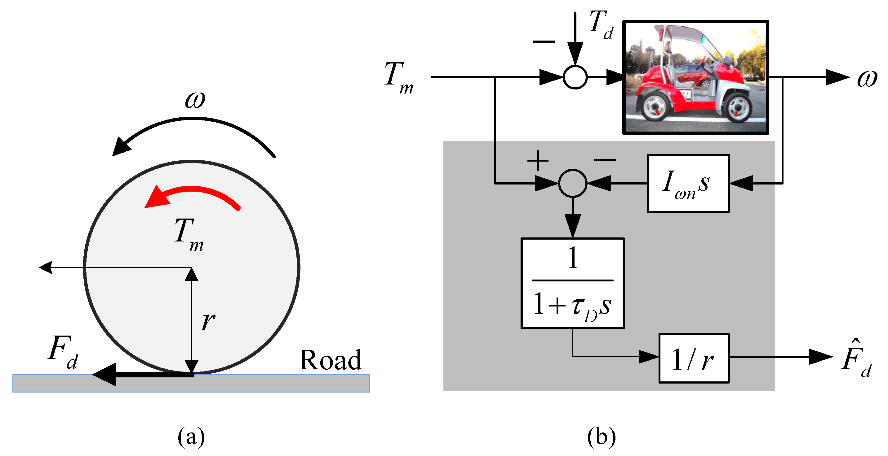
4.3. Design of a Driving Force Observer

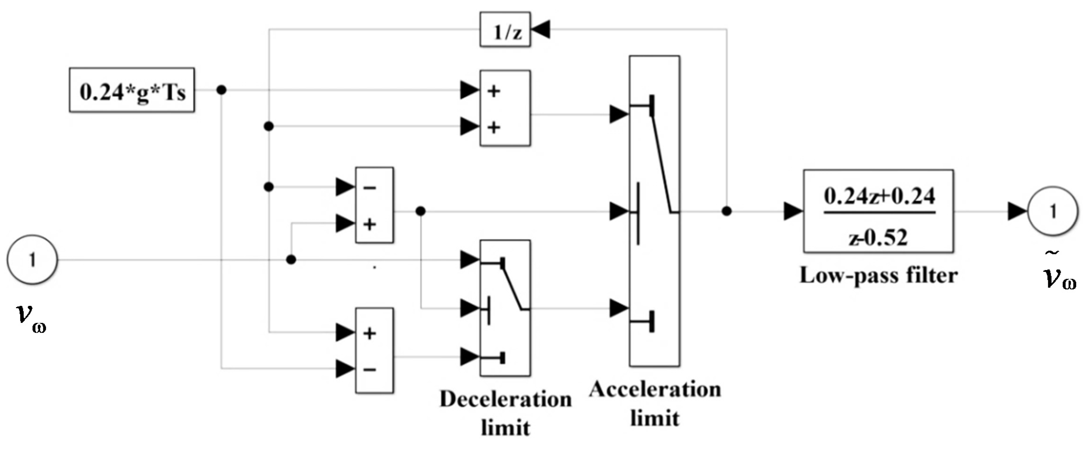
4.4. Vehicle Velocity Estimation
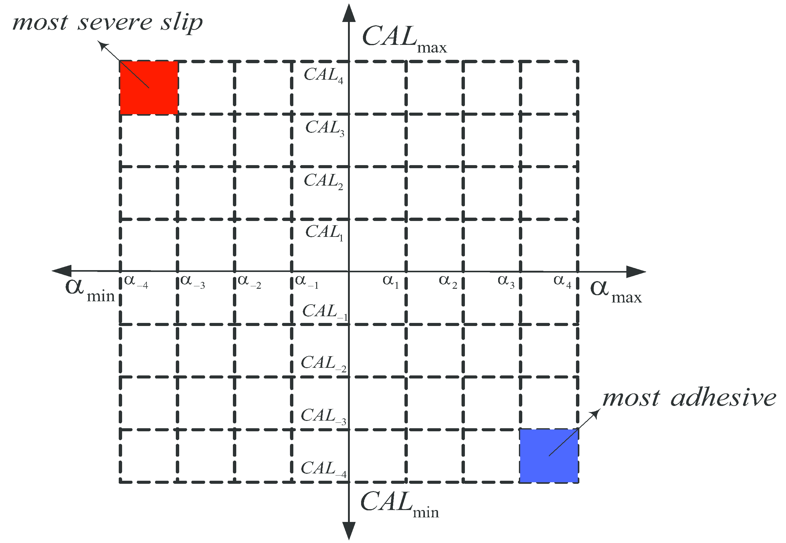
4.4.1. Design of a Wheel Slip Indicator
4.4.2. Wheel Acceleration Limiter and Rule-Based Logic

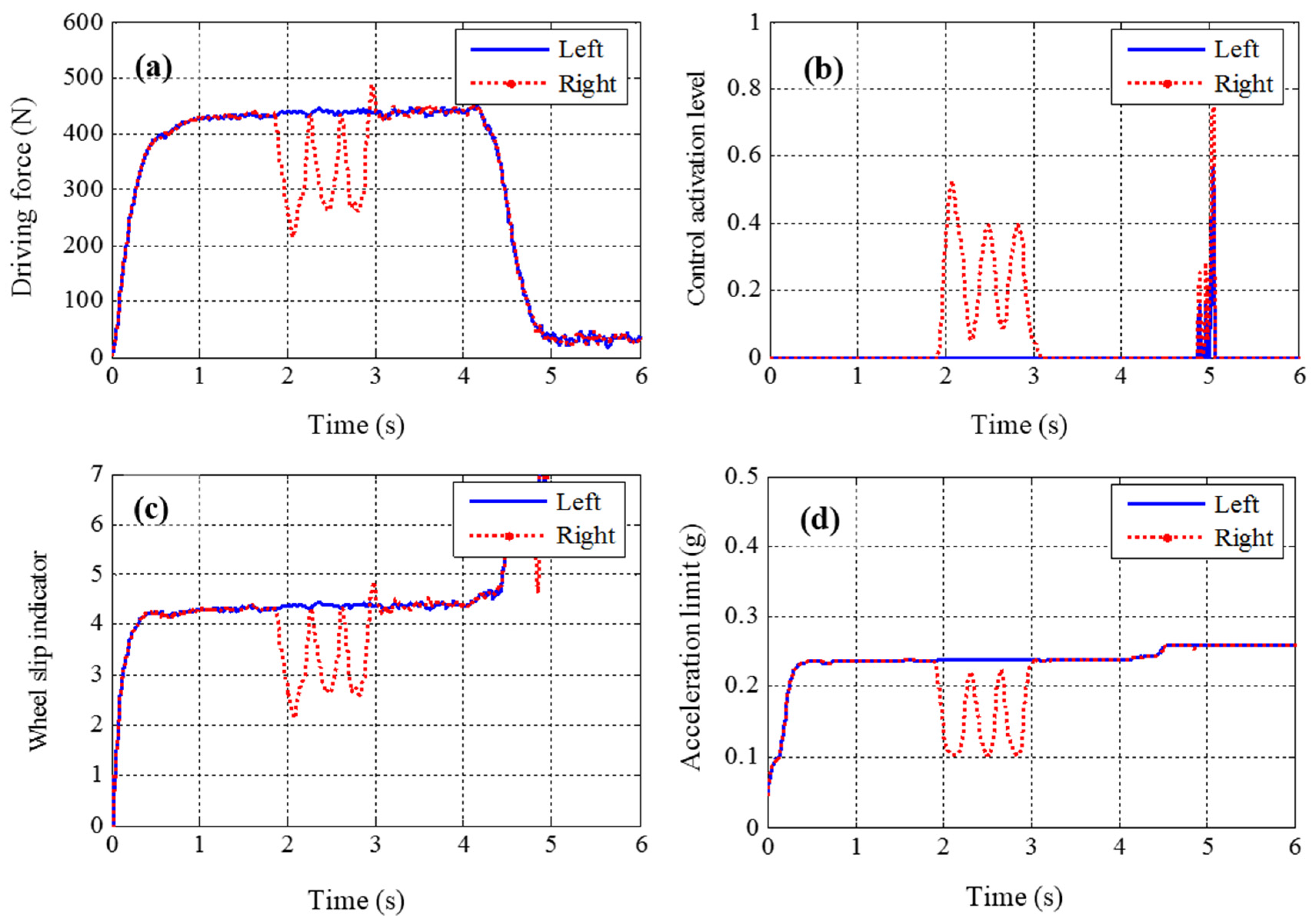
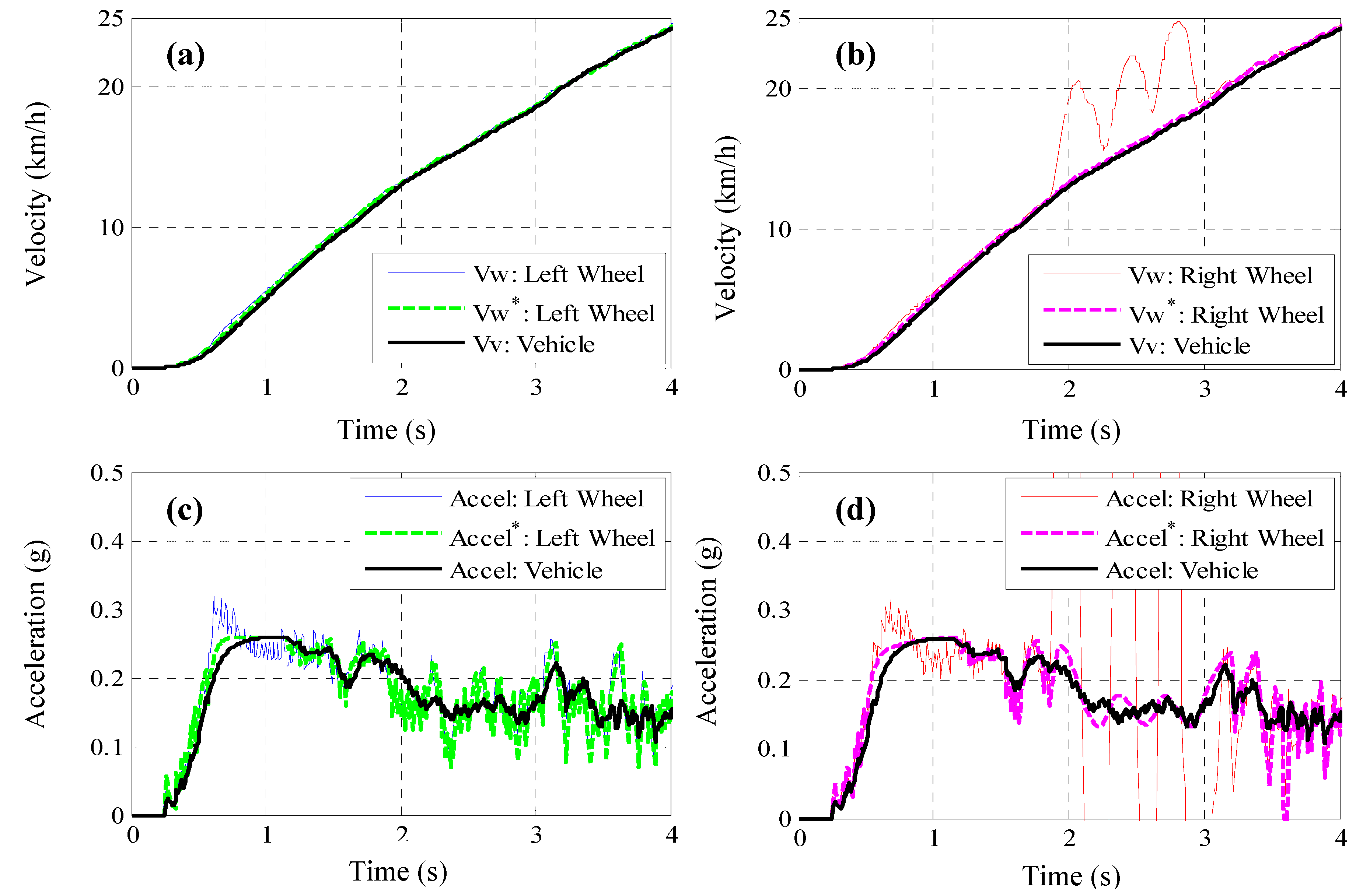
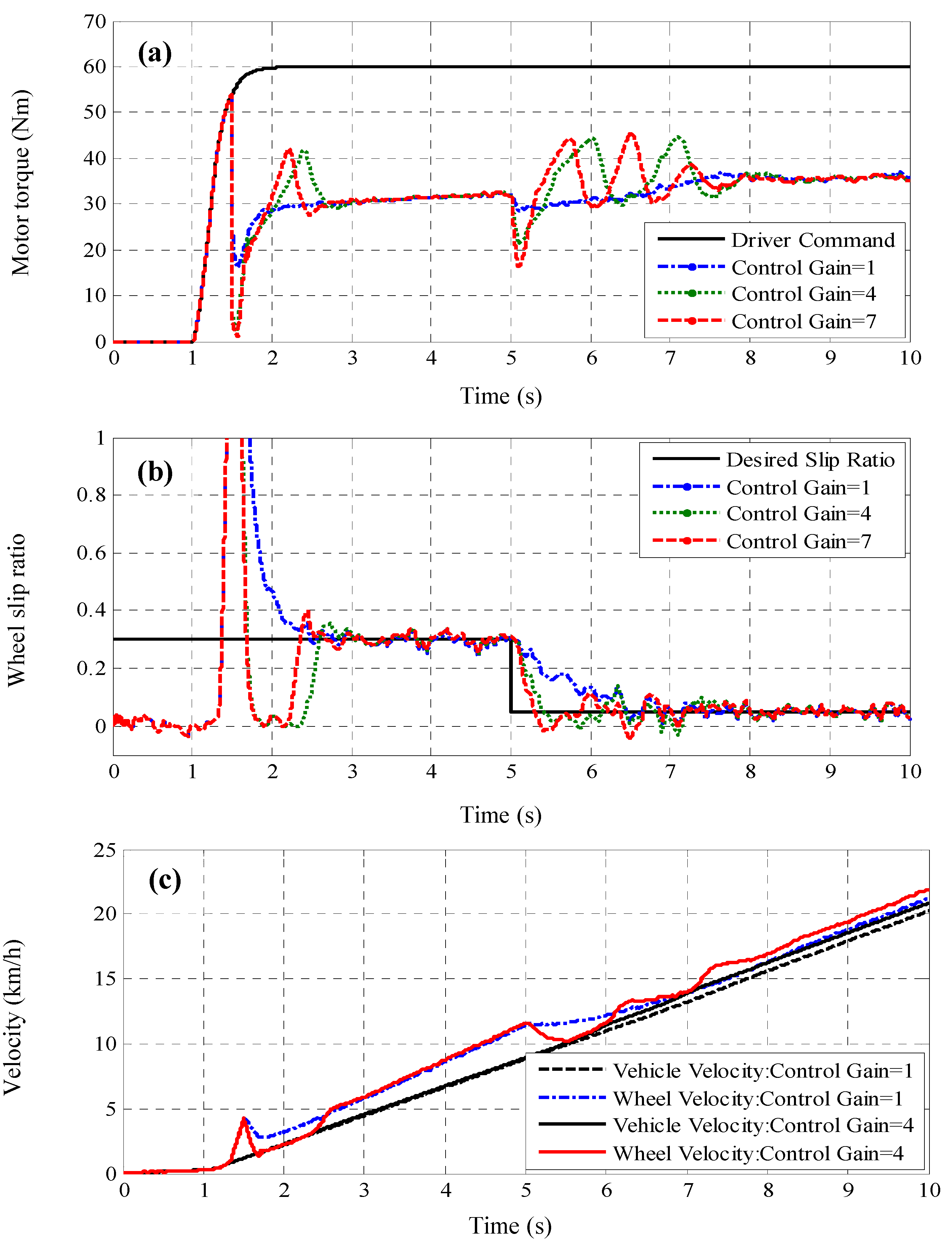
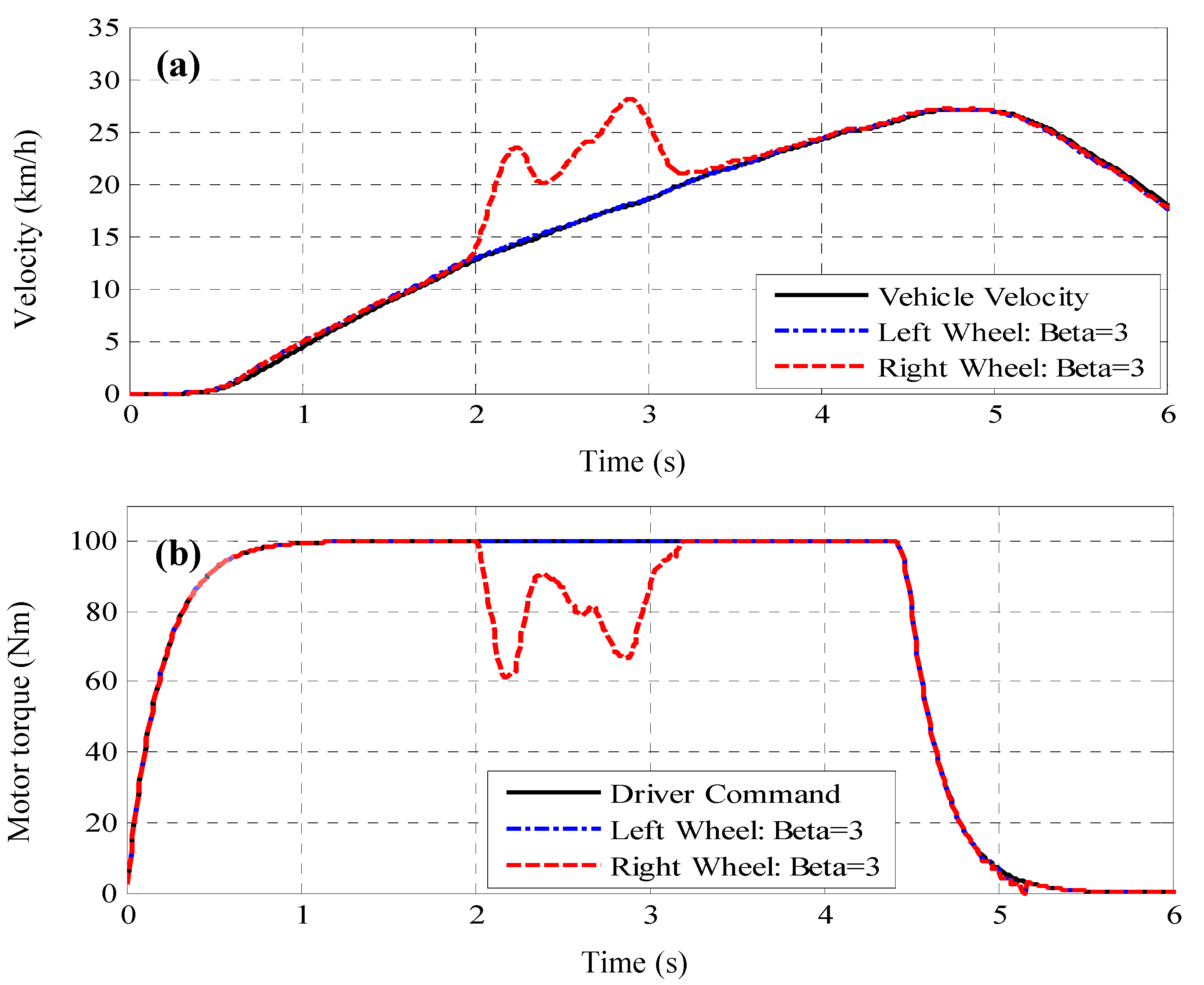
4.4.3. Experimental Results for Vehicle Velocity Estimation
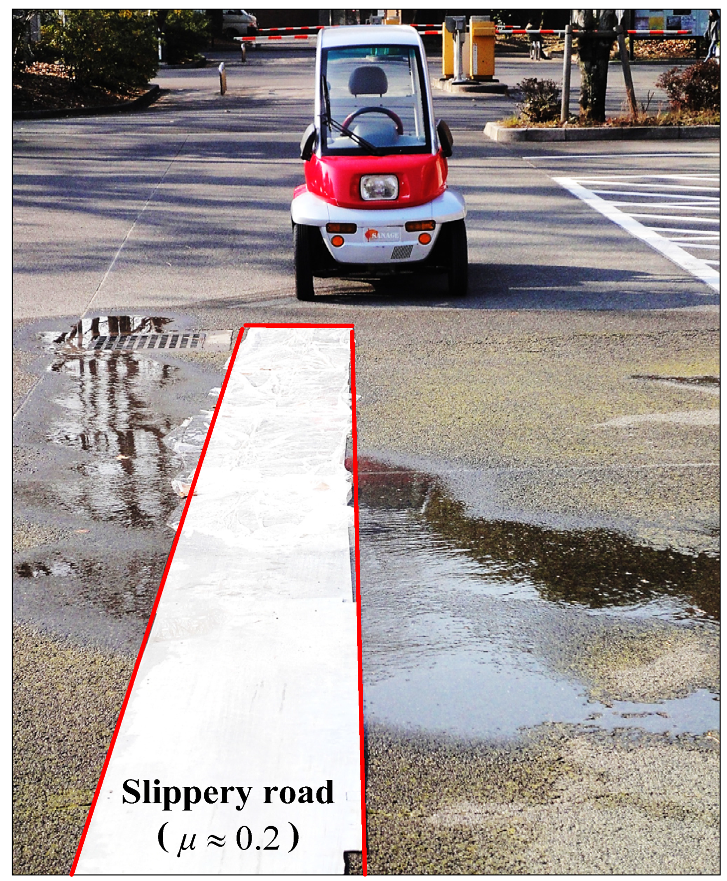
- Full acceleration without steering.
- Left wheel on high-µ surface and right wheel on high-µ/low-µ/high-µ transition surface.


5. Computer Simulation and Experimental Verification
5.1. Computer Simulation Using a CarSim Software
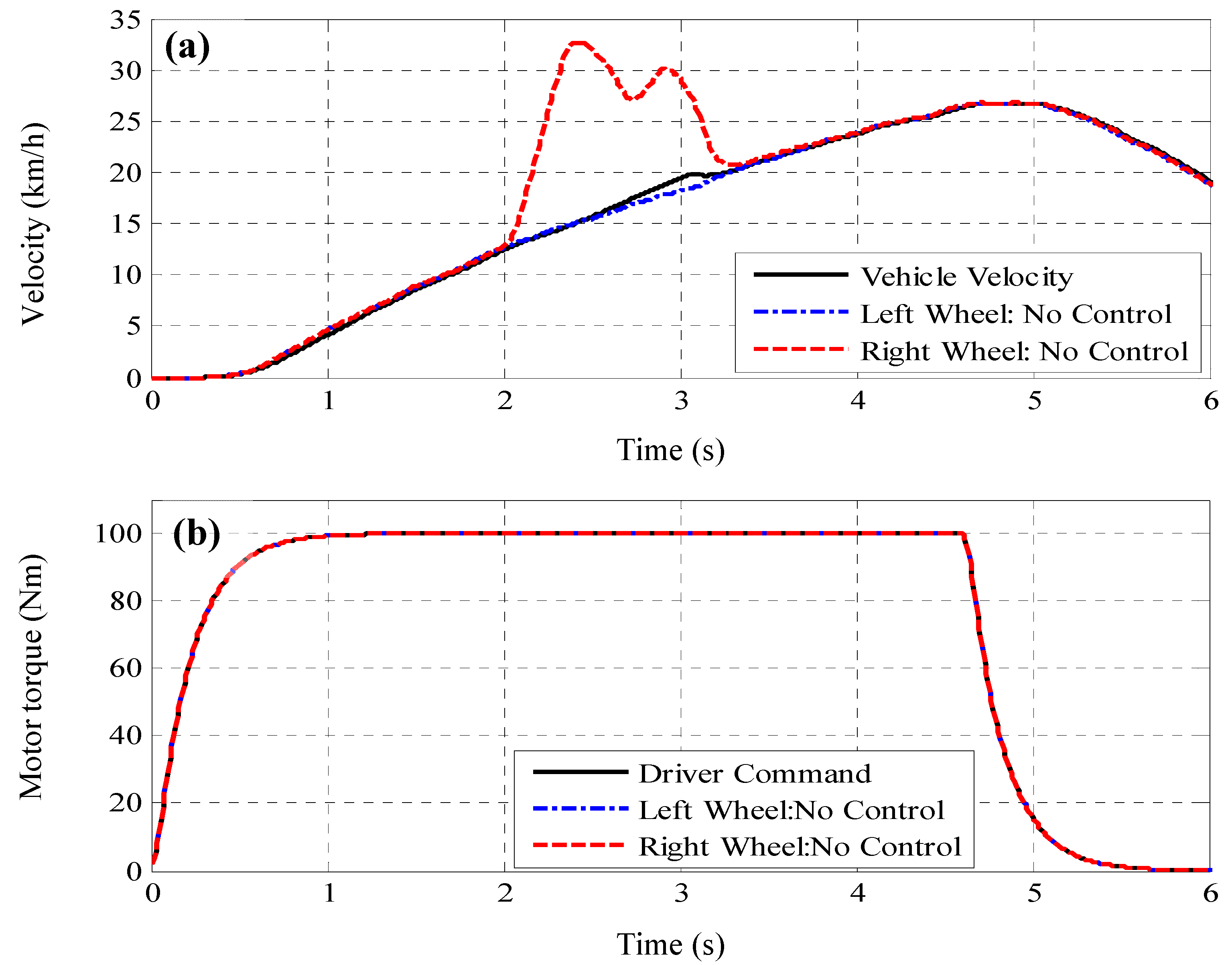
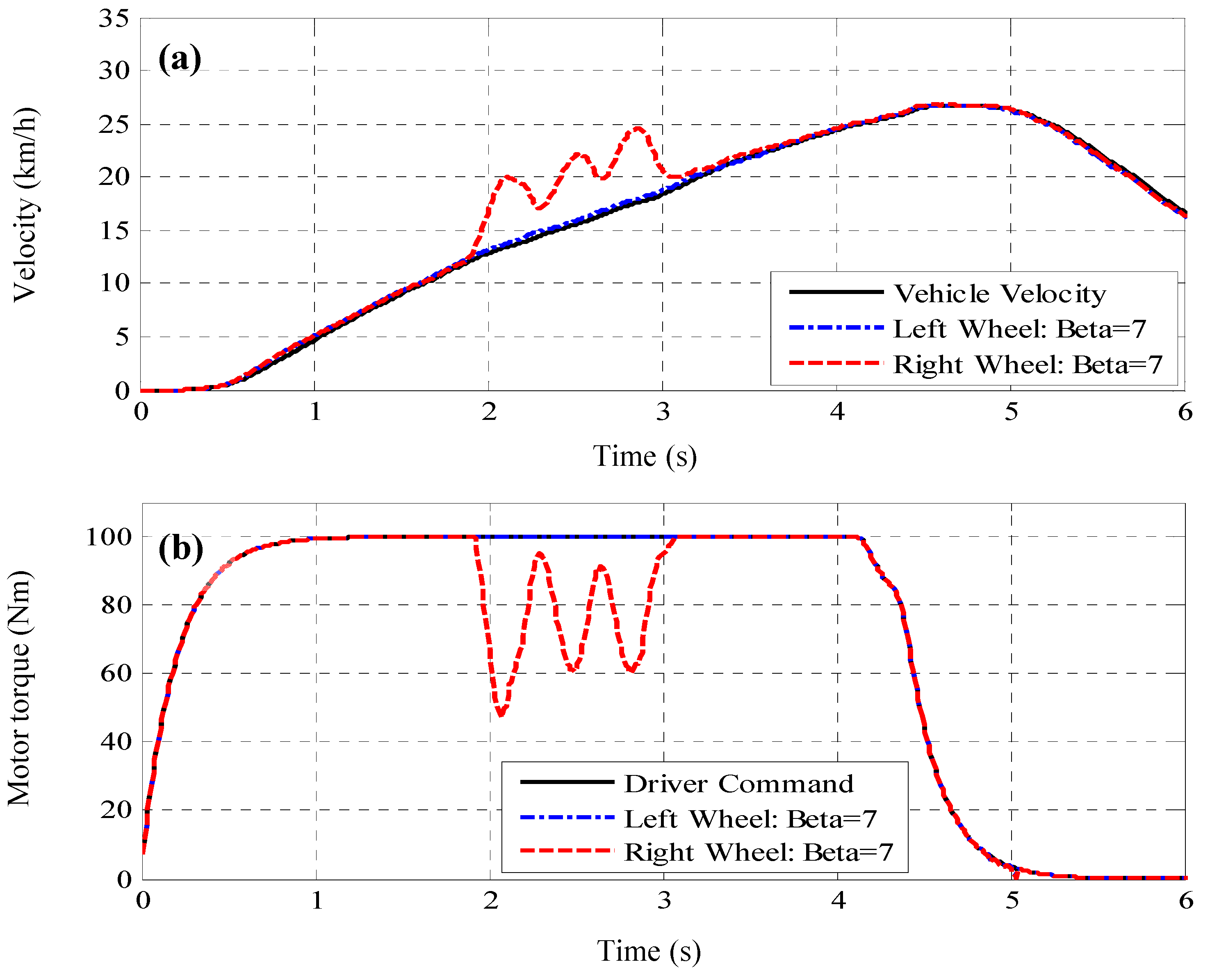
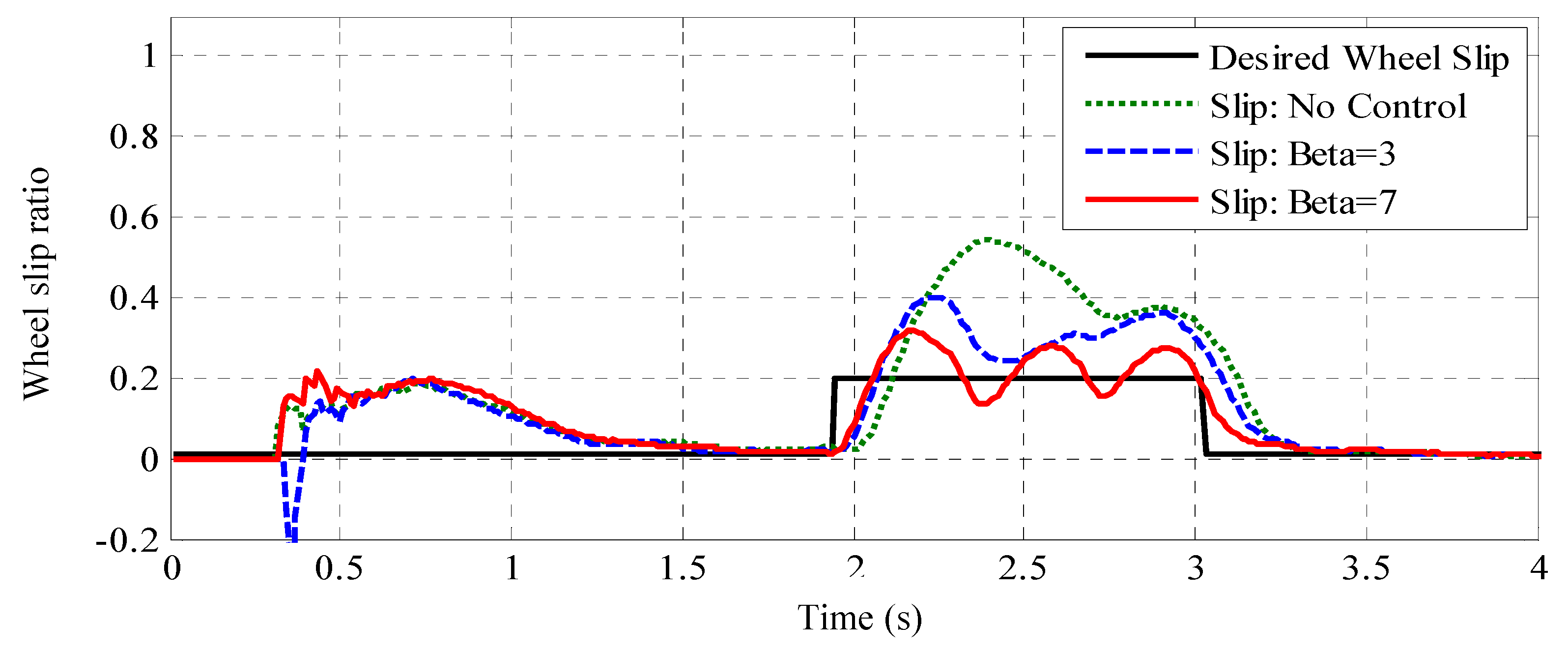
5.2. Experimental Verification


6. Conclusions
Acknowledgments
Author Contributions
Conflicts of Interest
References
- Fujimoto, H.; Fuji, K.; Takahashi, N. Traction and yaw-rate control of electric vehicle with slip-ratio and cornering stiffness estimation. In Proceedings of the American Control Conference, New York, NY, USA, 9–13 July 2007.
- Hori, Y.; Toyoda, Y.; Tsuruoka, Y. Traction control of electric vehicle: Basic experimental results using the test EV “UOT electric march”. IEEE Trans. Ind. Appl. 1998, 34, 1131–1138. [Google Scholar] [CrossRef]
- Sakai, S.; Sado, H.; Hori, Y. Motion control in an electric vehicle with four independently driven in-wheel motors. IEEE/ASME Trans. Mechatron. 1999, 4, 9–16. [Google Scholar] [CrossRef]
- Hori, Y. Future vehicle driven by electricity and control-research on four-wheel-motored “UOT electric march II”. IEEE Trans. Ind. Electron. 2004, 51, 954–962. [Google Scholar] [CrossRef]
- Dejun, Y.; Oh, S.; Hori, Y. A novel traction control for EV based on maximum transmissible torque estimation. IEEE Trans. Ind. Electron. 2009, 56, 2086–2094. [Google Scholar] [CrossRef]
- Deur, J.; Pavkovic, D.; Burgio, G.; Hrovat, D. A model-based traction control strategy non-reliant on wheel slip information. Veh. Syst. Dyn. 2011, 49, 1245–1265. [Google Scholar] [CrossRef]
- Magallan, G.A.; de Angelo, C.H.; Garcia, G.O. Maximization of the traction forces in a 2WD electric vehicle. IEEE Trans. Veh. Technol. 2011, 60, 369–380. [Google Scholar] [CrossRef]
- Yan, C.; Wang, J. Adaptive energy-efficient control allocation for planar motion control of over-actuated electric ground vehicles. IEEE Trans. Control Syst. Technol. 2014, 22, 1362–1373. [Google Scholar]
- Yin, G.; Wang, R.; Wang, J. Robust control for four wheel independently-actuated electric ground vehicles by external yaw-moment generation. Int. J. Automot. Technol. 2015, 16, 839–847. [Google Scholar] [CrossRef]
- Subudhi, B.; Ge, S.S. Sliding-mode-observer-based adaptive slip ratio control for electric and hybrid vehicles. IEEE Trans. Intell. Transp. Syst. 2012, 13, 1617–1626. [Google Scholar] [CrossRef]
- Mirzaeinejad, H.; Mirzaei, M. A novel method for non-linear control of wheel slip in anti-lock braking systems. Control Eng. Pract. 2010, 18, 918–926. [Google Scholar] [CrossRef]
- Amodeo, M.; Ferrara, A.; Terzaghi, R.; Vecchio, C. Wheel slip control via second-order sliding-mode generation. IEEE Trans. Intell. Transp. Syst. 2010, 11, 122–131. [Google Scholar] [CrossRef]
- Fazeli, A.; Zeinali, M.; Khajepour, A. Application of adaptive sliding mode control for regenerative braking torque control. IEEE/ASME Trans. Mechatron. 2012, 17, 745–755. [Google Scholar] [CrossRef]
- Castro, R.; Araujo, R.E.; Freitas, D. Wheel slip control of EVs based on sliding mode technique with conditional integrators. IEEE Trans. Ind. Electron. 2013, 60, 3256–3271. [Google Scholar] [CrossRef]
- He, H.; Peng, J.; Xiong, R.; Fan, H. An Acceleration slip regulation strategy for four-wheel drive electric vehicles based on sliding mode control. Energies 2014, 7, 3748–3763. [Google Scholar] [CrossRef]
- Johansen, T.A.; Petersen, I.; Kalkkuhl, J.; Ludemann, J. Gain-scheduled wheel slip control in automotive brake systems. IEEE Trans. Control Syst. Technol. 2003, 11, 799–811. [Google Scholar] [CrossRef]
- Savaresi, S.M.; Tanelli, M.; Cantoni, C. Mixed slip-deceleration control in automotive braking systems. J. Dyn. Syst. Meas. Control 2007, 129, 20–31. [Google Scholar] [CrossRef]
- Choi, S.B. Antilock brake system with a continuous wheel slip control to maximize the braking performance and the ride quality. IEEE Trans. Control Syst. Technol. 2008, 16, 996–1003. [Google Scholar] [CrossRef]
- Pasillas-Lepine, W.; Loria, A.; Gerard, M. Design and experimental validation of a nonlinear wheel slip control algorithm. Automatica 2012, 48, 1852–1859. [Google Scholar] [CrossRef]
- Mirzaei, M.; Mirzaeinejad, H. Optimal design of a non-linear controller for anti-lock braking system. Transp. Res. Part C Emerg. Technol. 2012, 24, 19–35. [Google Scholar] [CrossRef]
- Unsal, C.; Kachroo, P. Sliding mode measurement feedback control for antilock braking systems. IEEE Trans. Control Syst. Technol. 1999, 7, 271–281. [Google Scholar] [CrossRef]
- Goggia, T.; Sorniotti, A.; De Novellis, L.; Ferrara, A.; Gruber, P.; Theunissen, J.; Steenbeke, D.; Knauder, B.; Zehetner, J. Integral sliding mode for the torque-vectoring control of fully electric vehicles: Theoretical design and experimental assessment. IEEE Trans. Veh. Technol. 2015, 64, 1701–1715. [Google Scholar] [CrossRef]
- Gerard, M.; Pasillas-Lépine, W.; De Vries, E.; Verhaegen, M. Improvements to a five-phase ABS algorithm for experimental validation. Veh. Syst. Dyn. 2012, 50, 1585–1611. [Google Scholar] [CrossRef]
- Savaresi, S.M.; Tanelli, M. Active Braking Control Systems Design for Vehicles; Springer-Verlag: New York, NY, USA, 2010. [Google Scholar]
- Rajamani, R. Vehicle Dynamics and Control; Springer-Verlag: New York, NY, USA, 2005. [Google Scholar]
- Slotine, J.J.E.; Li, W. Applied Nonlinear Control; Prentice-Hall: Englewood Cliffs, NJ, USA, 1991. [Google Scholar]
- Nam, K.; Fujimoto, H.; Hori, Y. Design of an adaptive sliding mode controller for robust yaw stabilisation of in-wheel-motor-driven electric vehicles. Int. J. Veh. Des. 2015, 67, 98–113. [Google Scholar] [CrossRef]
- Nam, K.; Fujimoto, H.; Hori, Y. Lateral stability control of in-wheel-motor-driven electric vehicles based on sideslip angle estimation using lateral tire force sensors. IEEE Trans. Veh. Technol. 2012, 61, 1972–1985. [Google Scholar]
- Kobayashi, K.; Cheok, K.C.; Watanabe, K. Estimation of absolute vehicle speed using fuzzy logic rule-based Kalman filter. In Proceedings of the American Control Conference, Seattle, WA, USA, 21–23 June 1995; pp. 3086–3090.
- Daiss, A.; Kiencke, U. Estimation of vehicle speed fuzzy-estimation in comparison with Kalman-filtering. In Proceedings of the 4th IEEE Conference on Control Applications, New York, NY, USA, 28–29 September 1995.
- Jiang, F.; Gao, Z. An adaptive nonlinear filter approach to the vehicle velocity estimation for ABS. In Proceedings of the 2000 IEEE International Conference on Control Applications, Anchorage, AK, USA, 25–27 September 2000; pp. 490–495.
- Lars, I.; Tor, A.J.; Thor, I.F.; Håvard, F.G.; Jens, C.K.; Avshalom, S. Vehicle velocity estimation using nonlinear observers. Automatica 2006, 42, 2091–2103. [Google Scholar]
- Ljung, L. System Identification: Theory for the User; Prentice-Hall: Englewood Cliffs, NJ, USA, 1987. [Google Scholar]
© 2015 by the authors; licensee MDPI, Basel, Switzerland. This article is an open access article distributed under the terms and conditions of the Creative Commons Attribution license (http://creativecommons.org/licenses/by/4.0/).
Share and Cite
Nam, K.; Hori, Y.; Lee, C. Wheel Slip Control for Improving Traction-Ability and Energy Efficiency of a Personal Electric Vehicle. Energies 2015, 8, 6820-6840. https://doi.org/10.3390/en8076820
Nam K, Hori Y, Lee C. Wheel Slip Control for Improving Traction-Ability and Energy Efficiency of a Personal Electric Vehicle. Energies. 2015; 8(7):6820-6840. https://doi.org/10.3390/en8076820
Chicago/Turabian StyleNam, Kanghyun, Yoichi Hori, and Choonyoung Lee. 2015. "Wheel Slip Control for Improving Traction-Ability and Energy Efficiency of a Personal Electric Vehicle" Energies 8, no. 7: 6820-6840. https://doi.org/10.3390/en8076820
APA StyleNam, K., Hori, Y., & Lee, C. (2015). Wheel Slip Control for Improving Traction-Ability and Energy Efficiency of a Personal Electric Vehicle. Energies, 8(7), 6820-6840. https://doi.org/10.3390/en8076820