
Taxi Fleet Renewal in Cities with Improved Hybrid Powertrains: Life Cycle and Sensitivity Analysis in Lisbon Case Study

Abstract
:
1. Introduction
1.1. Road Vehicle Enhancements and Taxi Applications
1.2. Environmental and Financial Burden of Alternative Vehicles
1.3. Proposed Approach
2. Taxi Vehicle Simulation
2.1. Reference Taxi

| Component | Parameter | HEV a | ICEV b |
|---|---|---|---|
| Body | Curb weight (kg)/Cargo (kg) | 1368/70 | 1405/70 |
| Frontal area (m2)/Drag Coeficient | 2.16/0.25 | 2.5/0.28 | |
| Generator | Power (kW@rpm) | 44@1000–14000 rpm | - |
| Max Torque (N.m@rpm) | 40@1000 rpm | - | |
| Motor | Power (kW@rpm) | 60@14000 rpm | - |
| Max Torque (N.m@rpm) | 207@2500 rpm | - | |
| ICE | Nominal Power (kW@rpm) | 73@5200 rpm | 100 |
| Max Torque (N.m@rpm) | 142@4000 rpm | 270@2000/4200 rpm | |
| Battery | Energy capacity/Max. Power (kWh/kW) | 1.3/25 | - |
| Initial SOC | 60% | - | |
| Accessories | Power (W) | 1000 | 1000 |
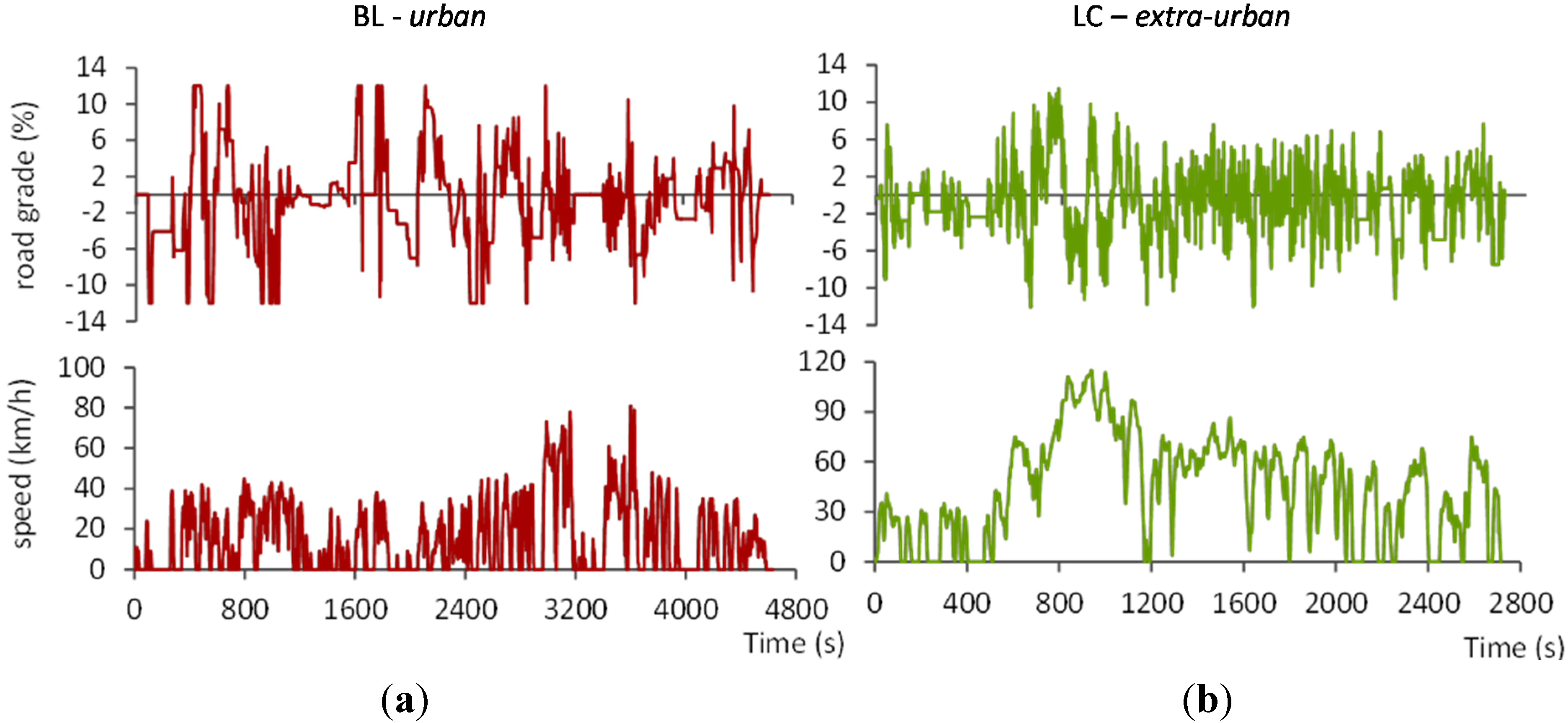
2.2. Driving Conditions

| Driving cycle | Time (s) | Distance (km) | Average speed (km/h) | Max. speed (km/h) | Average accel. (m/s2) | Max. accel./decel. (m/s2) | Max. VSP (W/kg) | # Stops | Grade |
|---|---|---|---|---|---|---|---|---|---|
| NEDC (synthetic) | 1184 | 10.9 | 33.2 | 120 | 0.54 | 1.06/−1.39 | 25.6 | 13 | No |
| WLTP (synthetic) | 1800 | 23.26 | 46.5 | 131 | 0.42 | 1.75/−1.48 | 30.1 | 8 | No |
| BL (urban) | 4630 | 20 | 15.5 | 81 | 0.81 | 4.44/−6.11 | 57.7 | 83 | Yes |
| LC (combined, with high extra-urban share) | 2705 | 34.2 | 45.5 | 115 | 0.69 | 3.89/−10.28 | 49.2 | 17 | Yes |
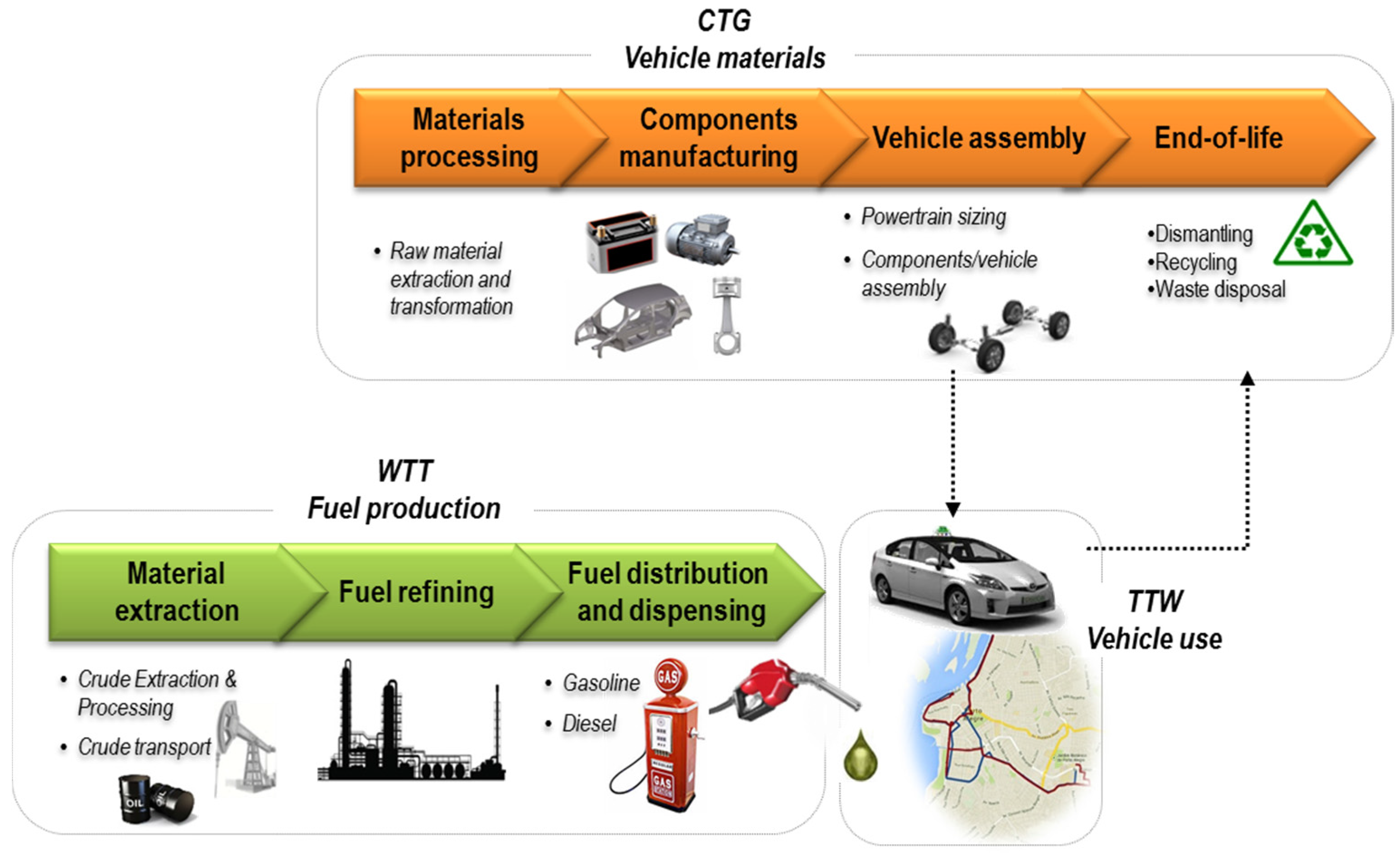
3. Life Cycle Environmental Analysis

| Energy k | Energy (MJ/MJfinal) yEk | CO2eq (g/MJfinal) yek | ||||
|---|---|---|---|---|---|---|
| Average | Min | Max | Average | Min | Max | |
| Diesel | 0.16 | 0.14 | 0.18 | 14.2 | 12.6 | 16 |
| Gasoline | 0.14 | 0.12 | 0.17 | 12.5 | 11.1 | 14.6 |
| Component j | Abbreviation | Energy (MJ/kgcomponent) zEi,j | CO2eq (gCO2eq/kgcomponent) zei,j |
|---|---|---|---|
| ICE system | ICE | 48.13 | 2840 |
| Motor & controller/generator | MC, GC | 159.09 | 10,094 |
| Battery (Lithium) | BAT | 224.71 | 13,438 |
| Battery (NiMh) | 205.15 | 11,719 |
3.1. Fuel Cycle—Well-to-Wheel
3.2. Materials Cycle—Cradle-to-Grave
| Components | Replacements (recommended service/km) |
|---|---|
| Pneumatics 1 | 1–10 (96,560–64,373) |
| Engine oil 1,2 | 23–133 (4828–8047) |
| Transmission oil 1 | 1 (average) |
| Brakes oil 1,2 | 2–25 (64,373–2 years) |
| Wind shield fluid 1 | 14–79 (51,206–18,170) |
| Powertrain Coolant 1,2 | 1–20 (80,467–3 years) |
| Lead-acid battery 3 | 2 (average) |
| Li-ion/NiMh battery 3 | 1–3 (28,1635–187,756) |
4. Financial Analysis
5. Optimization of the Hybrid Powertrain
5.1. Problem Formulation
| Optimization variables | Variables values range |
|---|---|
| ICEmodel | {1, 2, 3, 4} |
| ICEsize | [0.5, 2] |
| GCmodel | {1} |
| GCsize | [0.5, 2] |
| MCmodel | {1, 2, 3, 4} |
| MCsize | [0.5, 2] |
| BATmodel | {1, 2, 3, 4} |
| BATmodules | [5, 100] |
| Components | Components models | |||
|---|---|---|---|---|
| ICE model | ICE_1 a | ICE_2 b | ICE_3 c | ICE_4 d |
| Power (kW) | 43 | 73 | 66 | 50 |
| Weight (kg) | 137 | 173 | 158 | 130 |
| MC model | MC_1 e | MC_2 f | MC_3 g | MC_4 h |
| Power (kW) | 64 | 18 | 104 | 76 |
| Weight (kg) | 57 | 57 | 102 | 57 |
| GC model | GC_1 i | |||
| Power (kW) | 38 | |||
| Weight (kg) | 33 | |||
| BAT model | BAT_1 j | BAT_2 k | BAT_3 l | BAT_4 m |
| Min./Max. voltage (V) | 2.5/4.1 | 2.7/4.2 | 6/9 | 10.25/14 |
| Capacity (Ah) | 7 | 40 | 5.5 | 34 |
| Weight (kg) | 0.35 | 1 | 1.04 | 9 |
| Type | Cell | Cell | Module | Module |
| Chemistry | Li-ion | Li-ion | NiMh | NiMh |
5.2. Multi-Objective Optimization Algorithm

- (1)
- Initially, a random parent population of size n individuals, is created, P0.
- (2)
- The population is evaluated and sorted based on the non-domination concept.
- (3)
- A combined population Rt with the size of 2n is formed: Rt = Pt ∪ Qt.
- (4)
- A generation is complete, and now the new population Pt+1 become a parent population and the process is repeated. The final non-dominated set, the Pareto front, is achieved if one of the stopping criteria is reached: maximum number of generations (200), or if an average change in the spread of the Pareto front over a specified number of generations (150) is less than a specified tolerance (0.001).
5.3. Multi Criteria Score Approach
6. Results and Discussion


| ICE | MC | GC | BAT | Vehicle mass | ||||||||||
|---|---|---|---|---|---|---|---|---|---|---|---|---|---|---|
| Model * | Size * | (kW) | Model * | Size * | (kW) | Size * | (kW) | Model * | Modules * | (kW) | (kWh) | (kg) | ||
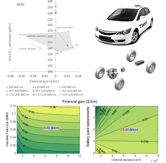
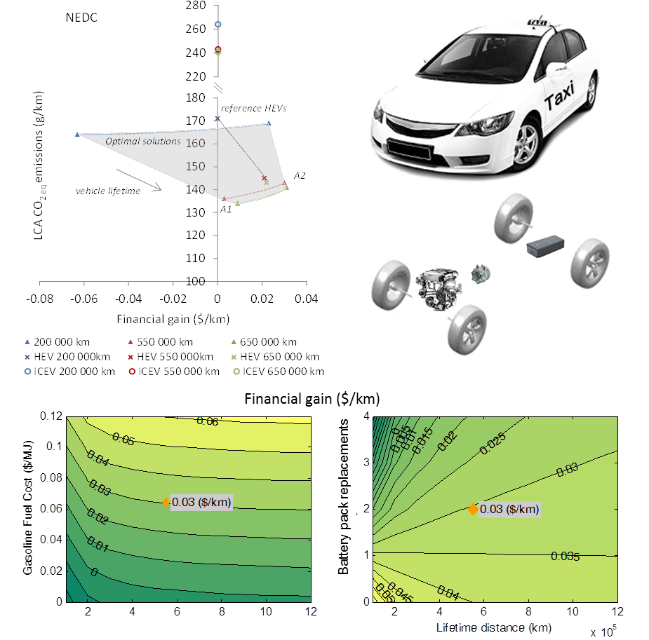
| NEDC | A1 | 2 | 0.70 | 51 | 1 | 0.96 | 61 | 0.58 | 22 | 2 (Li-ion) | 69 | 145 | 9.9 | 1408 |
| A2 | 2 | 0.69 | 50 | 1 | 0.72 | 46 | 0.51 | 19 | 3 (NiMh) | 59 | 56 | 2.5 | 1384 | |
| BL | B1 | 2 | 0.89 | 64 | 3 | 0.75 | 78 | 0.74 | 28 | 4 (NiMh) | 59 | 310 | 24.5 | 1924 |
| B2 | 2 | 1.09 | 79 | 1 | 1.51 | 96 | 0.81 | 30 | 4 (NiMh) | 42 | 221 | 17.5 | 1813 | |
| B3 | 2 | 1.48 | 107 | 1 | 1.75 | 112 | 1.18 | 44 | 3 (NiMh) | 78 | 74 | 3.3 | 1601 | |
| LC | C1 | 2 | 0.73 | 54 | 1 | 1.08 | 69 | 1.36 | 51 | 2 (Li-ion) | 70 | 148 | 10.1 | 1449 |
| C2 | 2 | 0.79 | 57 | 3 | 0.55 | 57 | 1.32 | 50 | 3 (NiMh) | 47 | 44 | 1.9 | 1427 | |
| Life cycle energy use (LE) and CO2eq emissions (Le) | |||||||||||||||||||
|---|---|---|---|---|---|---|---|---|---|---|---|---|---|---|---|---|---|---|---|
| Driving cycle | Vehicle | 200,000 kmlifetime | 550,000 kmlifetime | 650,000 kmlifetime | |||||||||||||||
| LE (MJ/km) | Le (g/km) | LE (MJ/km) | Le (g/km) | LE (MJ/km) | Le (g/km) | ||||||||||||||
| av. | min | max | av. | min | max | av. | min | max | av. | min | max | av. | min | max | av. | min | max | ||
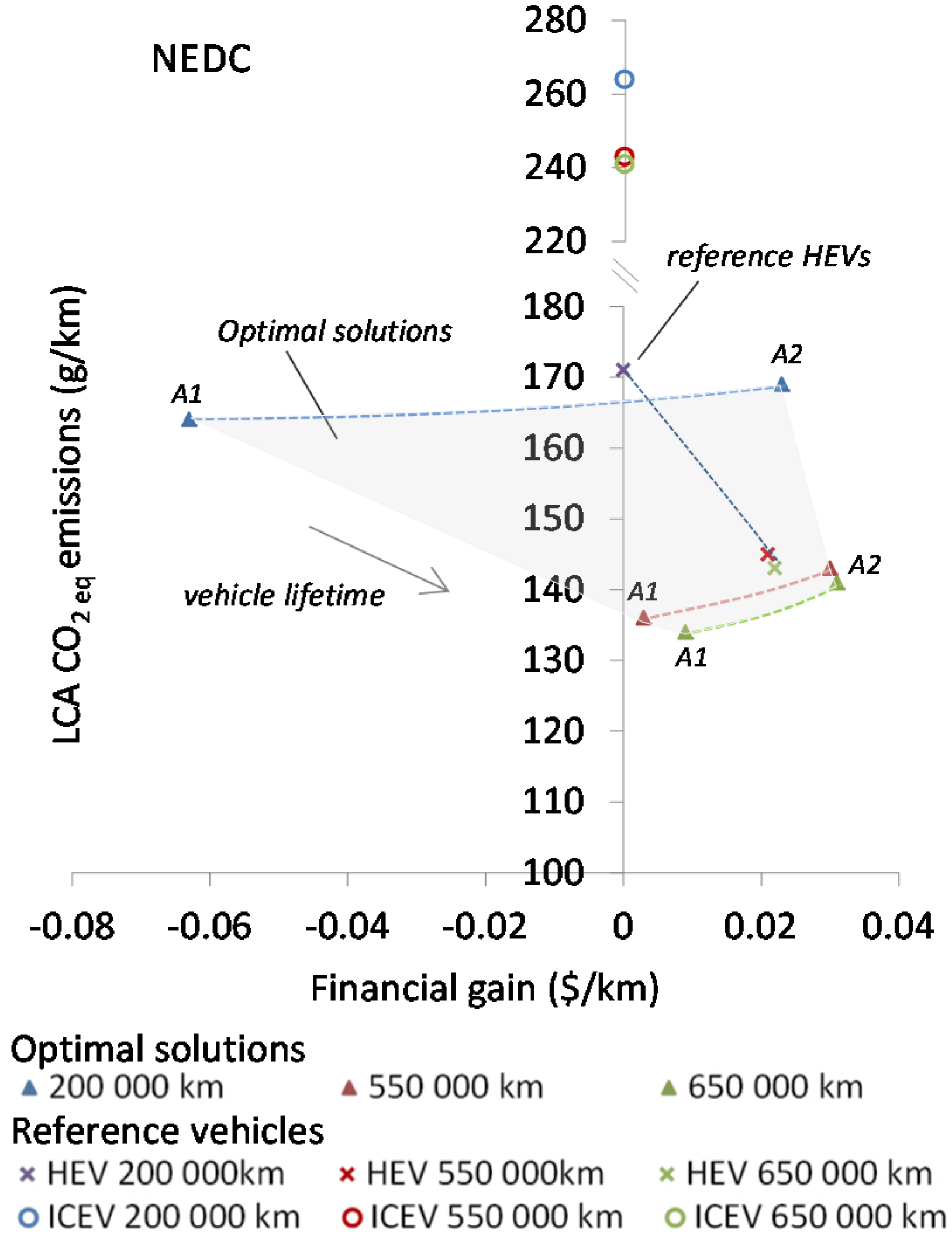
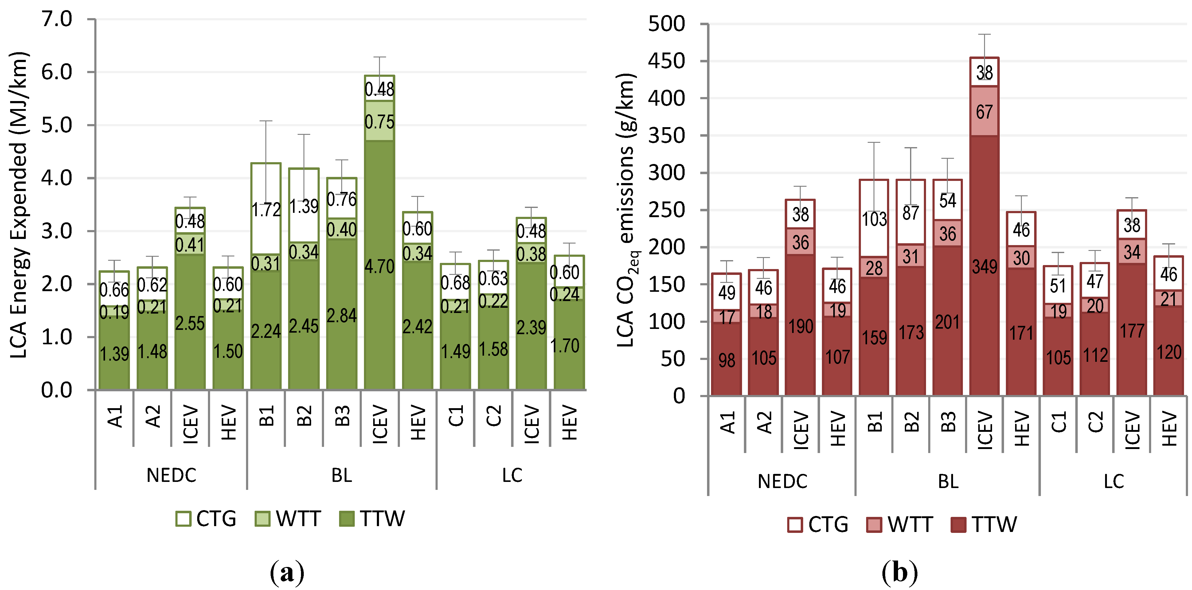
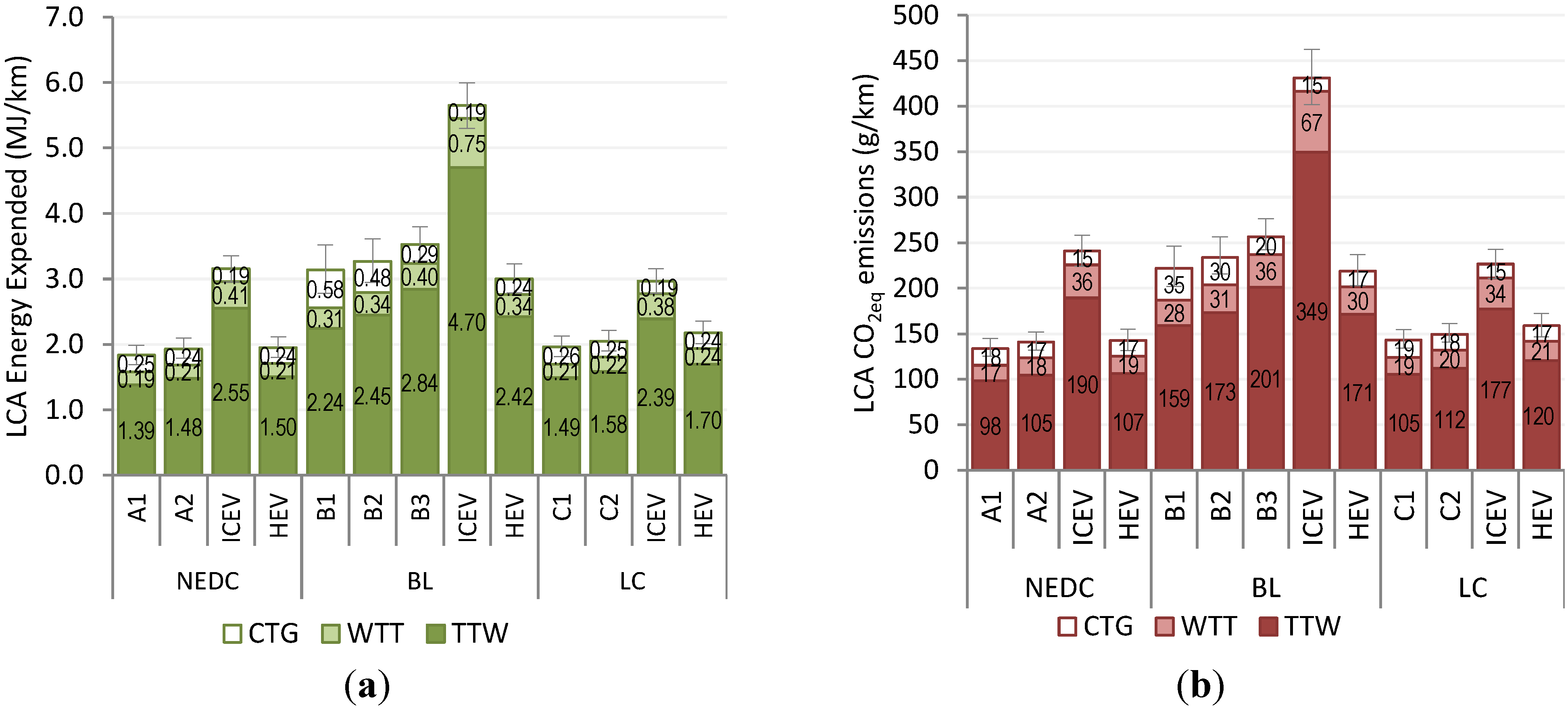
| NEDC | A1 | 2.23 | 2.04 | 2.45 | 164 | 153 | 182 | 1.86 | 1.72 | 2.02 | 136 | 127 | 147 | 1.83 | 1.69 | 1.99 | 134 | 125 | 145 |
| A2 | 2.31 | 2.12 | 2.52 | 169 | 158 | 186 | 1.96 | 1.81 | 2.12 | 143 | 134 | 154 | 1.93 | 1.79 | 2.09 | 141 | 132 | 152 | |
| HEV | 2.31 | 2.11 | 2.53 | 171 | 157 | 187 | 1.97 | 1.82 | 2.14 | 145 | 134 | 157 | 1.95 | 1.80 | 2.11 | 143 | 132 | 155 | |
| ICEV | 3.44 | 3.24 | 3.64 | 264 | 248 | 282 | 3.18 | 2.98 | 3.38 | 243 | 226 | 260 | 3.15 | 2.95 | 3.35 | 241 | 224 | 258 | |
| BL | B1 | 4.28 | 3.51 | 5.08 | 290 | 249 | 341 | 3.23 | 2.84 | 3.64 | 227 | 206 | 253 | 3.14 | 2.78 | 3.52 | 222 | 202 | 246 |
| B2 | 4.18 | 3.57 | 4.82 | 290 | 257 | 334 | 3.34 | 3.00 | 3.71 | 238 | 219 | 262 | 3.27 | 2.95 | 3.61 | 234 | 216 | 256 | |
| B3 | 4.00 | 3.69 | 4.34 | 290 | 273 | 319 | 3.56 | 3.31 | 3.84 | 259 | 245 | 279 | 3.52 | 3.28 | 3.80 | 257 | 242 | 276 | |
| HEV | 3.36 | 3.09 | 3.65 | 247 | 229 | 269 | 3.02 | 2.81 | 3.26 | 221 | 205 | 239 | 3.00 | 2.78 | 3.23 | 219 | 203 | 237 | |
| ICEV | 5.93 | 5.58 | 6.29 | 454 | 425 | 486 | 5.67 | 5.32 | 6.02 | 433 | 404 | 464 | 5.65 | 5.30 | 6.00 | 431 | 402 | 462 | |
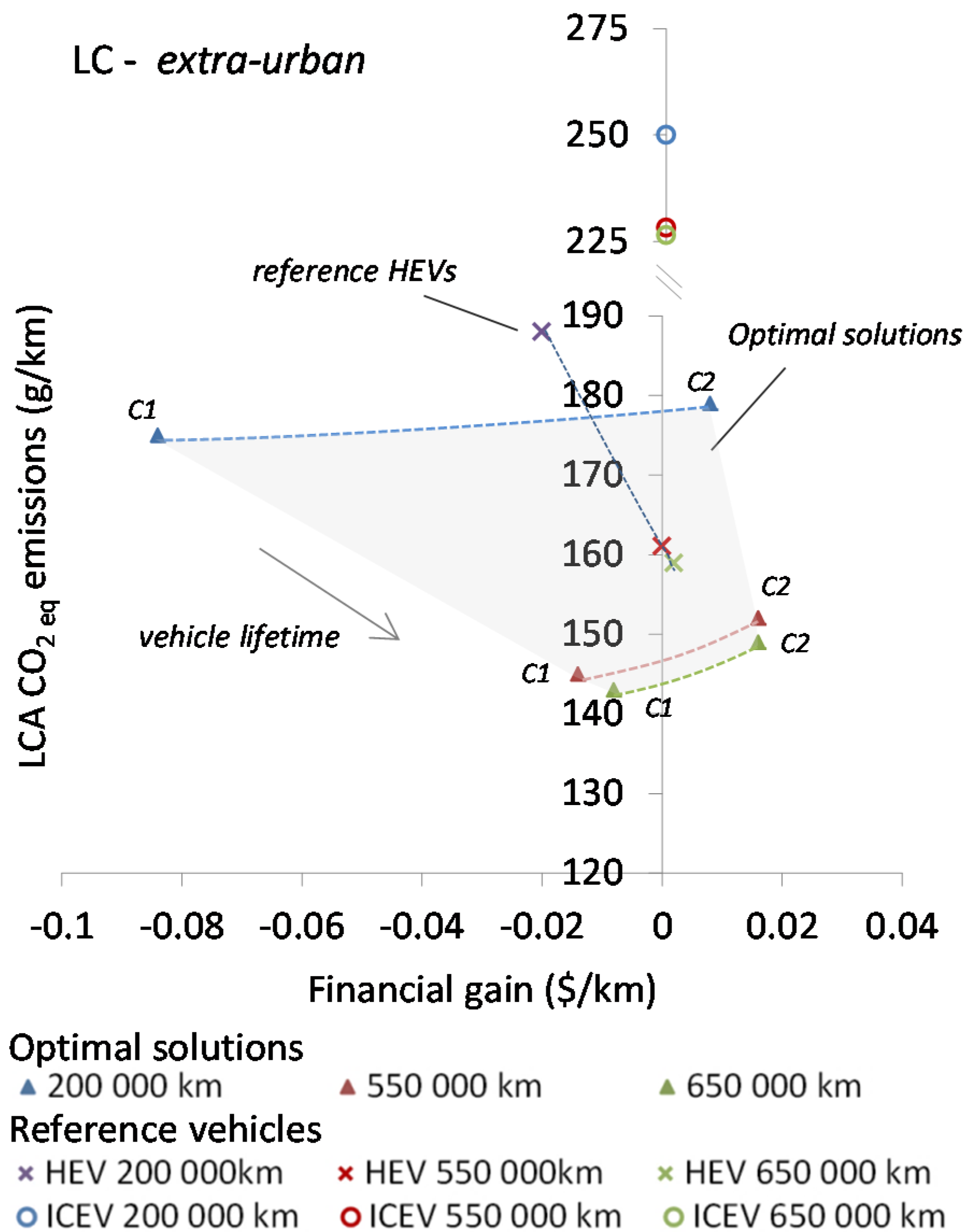
| LC | C1 | 2.38 | 2.18 | 2.61 | 175 | 163 | 193 | 1.99 | 1.84 | 2.16 | 145 | 136 | 157 | 1.96 | 1.81 | 2.12 | 143 | 134 | 155 |
| C2 | 2.44 | 2.25 | 2.64 | 179 | 168 | 196 | 2.08 | 1.93 | 2.25 | 152 | 143 | 163 | 2.05 | 1.90 | 2.21 | 149 | 141 | 161 | |
| HEV | 2.54 | 2.32 | 2.77 | 188 | 173 | 204 | 2.20 | 2.04 | 2.39 | 161 | 149 | 175 | 2.18 | 2.01 | 2.35 | 159 | 147 | 172 | |
| ICEV | 3.25 | 3.06 | 3.45 | 250 | 234 | 267 | 2.99 | 2.81 | 3.18 | 228 | 213 | 245 | 2.97 | 2.78 | 3.15 | 226 | 211 | 243 | |
| Driving cycle | Vehicle | Powertrain cost ($) | Financial gain (Fg) ($/kmlifetime) | ||
|---|---|---|---|---|---|
| 200,000 kmlifetime | 550,000 kmlifetime | 650,000 kmlifetime | |||
| NEDC | A1 | 27,804 | −0.063 | 0.003 | 0.009 |
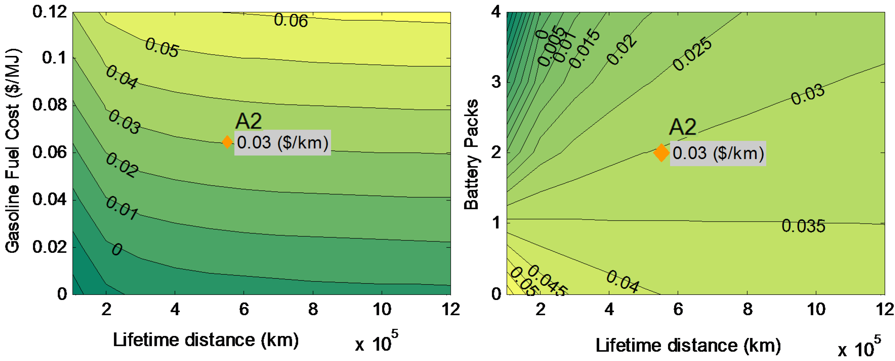
| A2 | 9506 | 0.023 | 0.030 | 0.031 | |
| HEV | 13,793 | 0 | 0.021 | 0.022 | |
| ICEV | 7072 | - | - | - | |
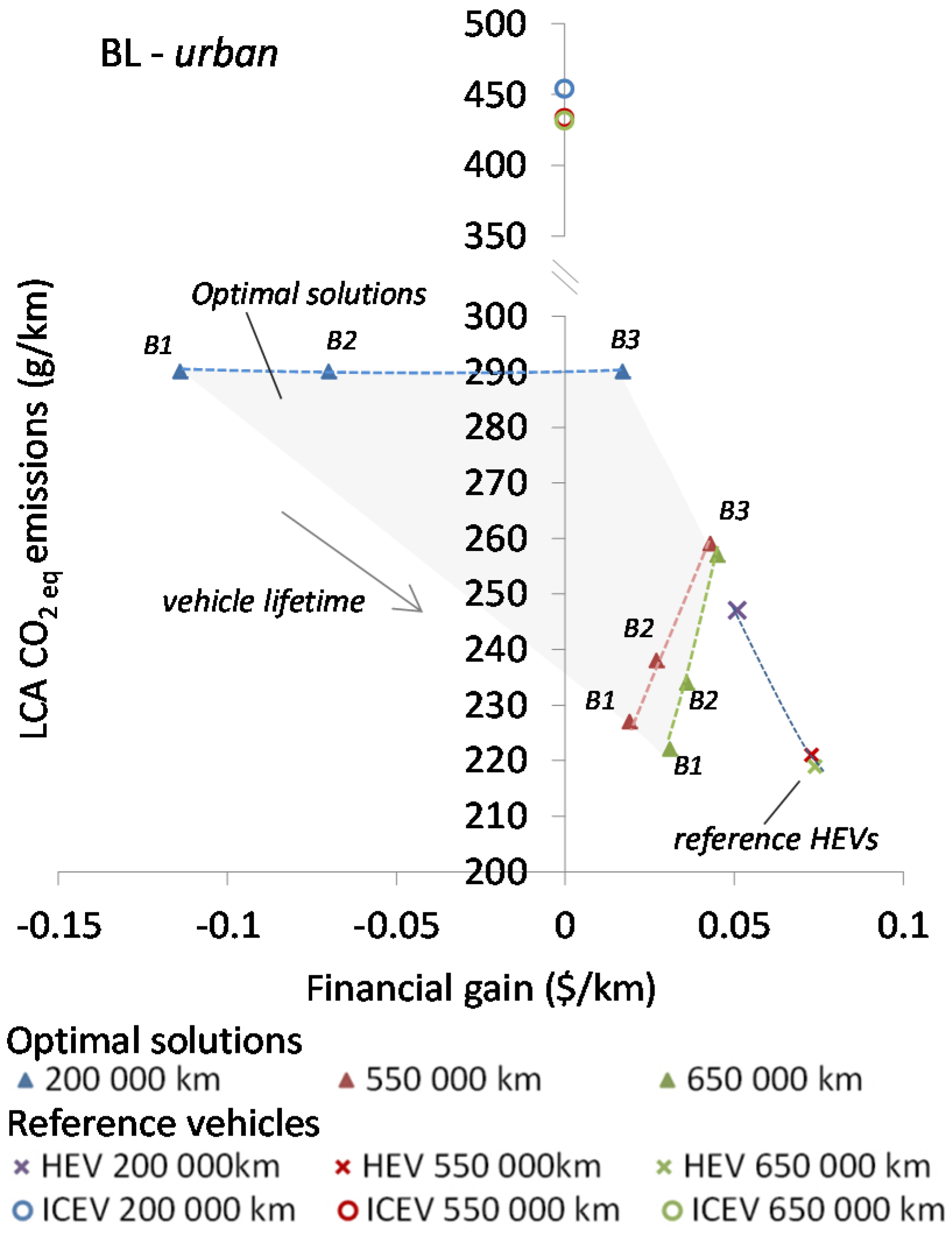
| BL | B1 | 49,031 | −0.114 | 0.019 | 0.031 |
| B2 | 37,541 | −0.070 | 0.027 | 0.036 | |
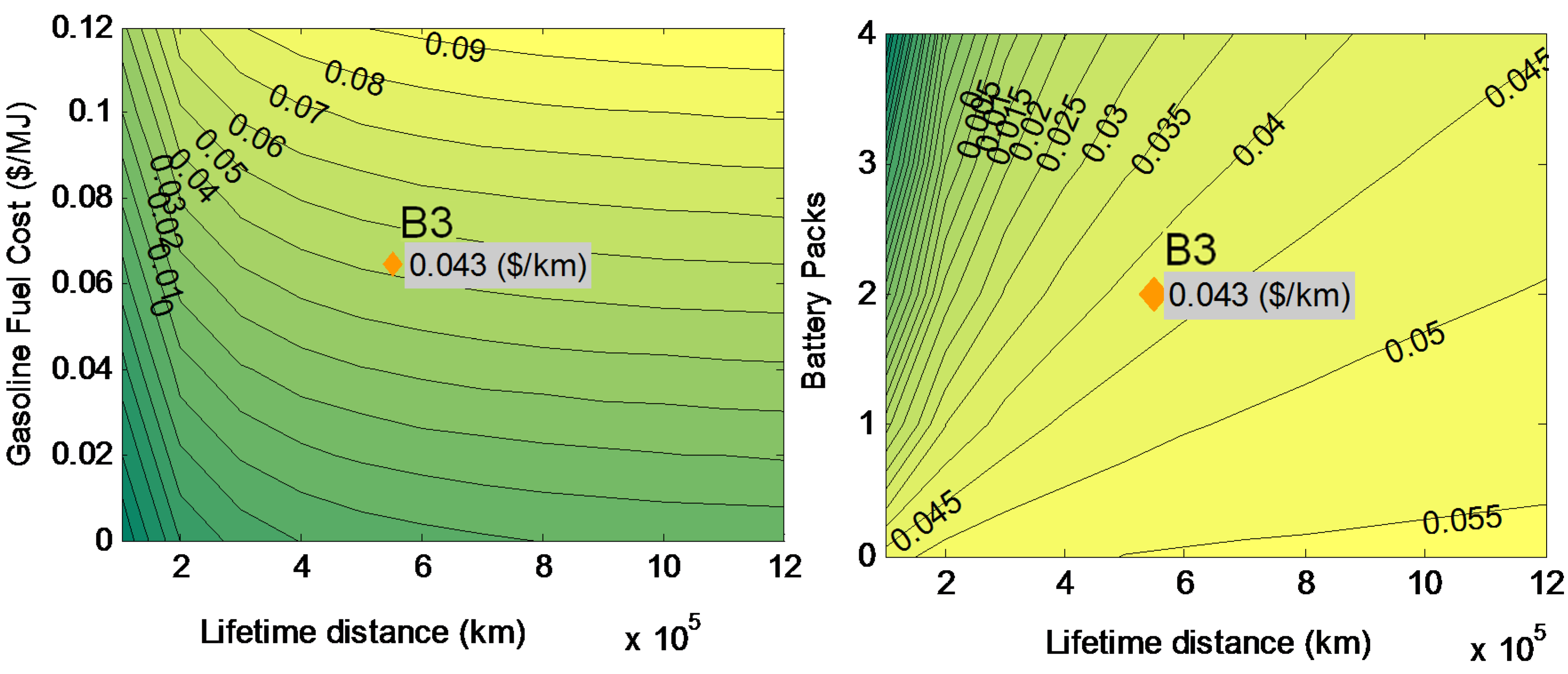
| B3 | 14,964 | 0.017 | 0.043 | 0.045 | |
| HEV | 13,793 | 0.051 | 0.073 | 0.074 | |
| ICEV | 7072 | - | - | - | |
| LC | C1 | 29,100 | −0.084 | −0.014 | −0.008 |
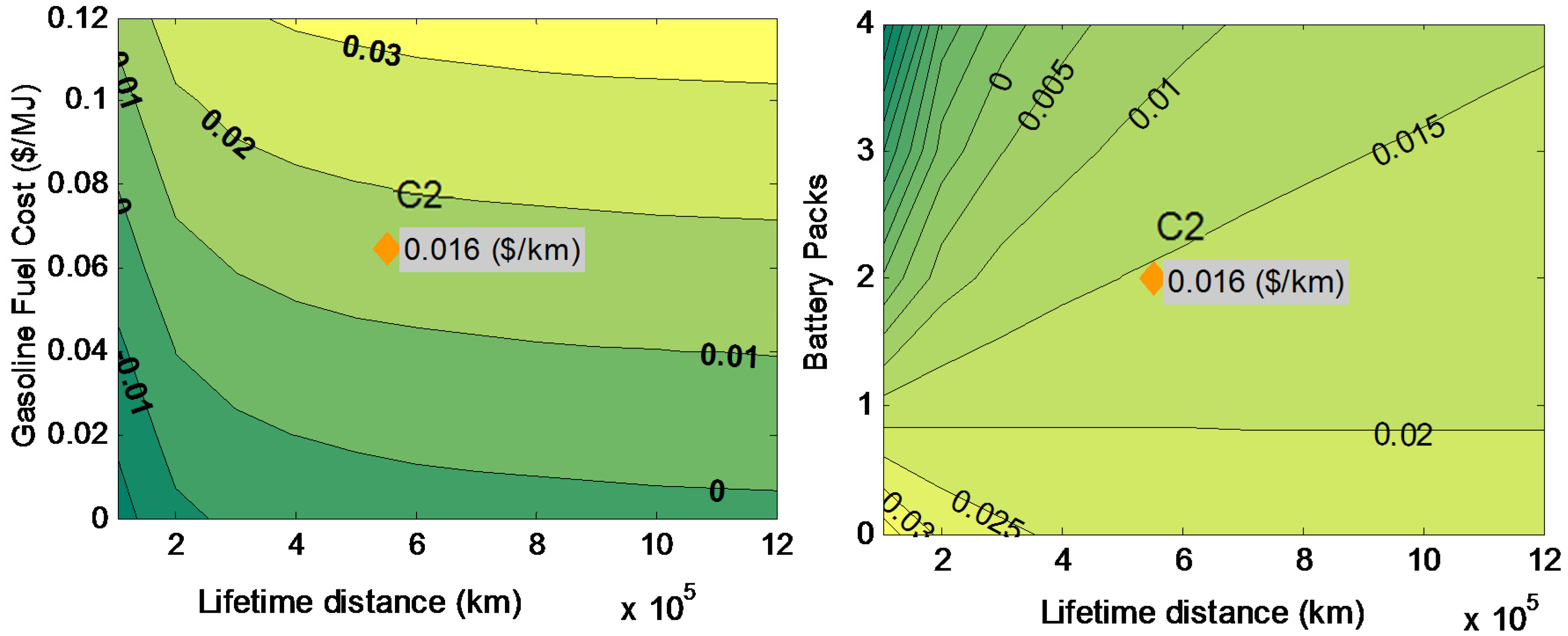
| C2 | 9501 | 0.008 | 0.016 | 0.016 | |
| HEV | 13,793 | −0.02 | 0 | 0.002 | |
| ICEV | 7072 | - | - | - | |


| BL | LC | WLTP | |||||||
|---|---|---|---|---|---|---|---|---|---|
| TTW (MJ/km) | Le (g/km) | Fg ($/km) | TTW (MJ/km) | Le (g/km) | Fg ($/km) | TTW (MJ/km) | Le (g/km) | Fg ($/km) | |
| ICEV | 4.70 | 433 | - | 2.39 | 228 | - | 2.37 | 227 | - |
| HEV | 2.42 | 221 | 0.073 | 1.70 | 161 | 0 | 1.59 | 155 | 0.002 |
| B1 | 2.24 | 227 | 0.019 | 1.97 | 190 | −0.082 | 2.23 | 205 | −0.099 |
| B2 | 2.45 | 238 | 0.027 | 2.19 | 201 | −0.075 | 2.15 | 193 | −0.073 |
| B3 | 2.84 | 259 | 0.044 | 2.48 | 214 | −0.052 | 2.41 | 201 | −0.049 |
| C1 | 1.73 | 150 | 0.089 | 1.49 | 145 | −0.014 | 1.52 | 134 | −0.017 |
| C2 | 2.20 | 188 | 0.094 | 1.58 | 152 | 0.016 | 1.58 | 137 | 0.016 |
| Vehicle | Veh. cost | Total of points (BL, LC and WLTP) | Ranking | |||
|---|---|---|---|---|---|---|
| TTW | Le | Fg | Total score | |||
| HEV | 5 (#2) | 14 (#3) | 15 (#3) | 17 (#2) | 42 | #3 |
| B1 | 1 (#6) | 12 (#4) | 10 (#4) | 2 (#6) | 18 | #4 |
| B2 | 2 (#5) | 10 (#5) | 10 (#4) | 3 (#5) | 18 | #5 |
| B3 | 4 (#4) | 6 (#6) | 7 (#6) | 4 (#4) | 14 | #6 |
| C1 | 3 (#3) | 21 (#1) | 21 (#1) | 6 (#3) | 44 | #2 |
| C2 | 6 (#1) | 18 (#2) | 18 (#2) | 21 (#1) | 54 | #1 |
7. Conclusions
Acknowledgments
Author Contributions
Conflicts of Interest
Appendix A


References
- European Road Transport Research Advisory Council (ERTRAC). Available online: http://cordis.europa.eu/technology-platforms/ertrac_en.html (accessed on 11 April 2014).
- European Commision, Directive 2003/30/EC of the European Parliament and of the Council of 8 May 2003 on the promotion of the use of biofuels or other renewable fuels for transport. Off. J. Eur. Union 2003, 4, 42–46. Available online: http://eur-lex.europa.eu/legal-content/EN/TXT/?uri=celex:32003L0030 (accessed on 11 April 2015).
- Edwards, R.; Mahieu, V.; Griesemann, J.; Larivé, J. Well-to-Wheels Analysis of future Automotive Fuels and Powertrains in The European Context; WELL-to-TANK Report Version 3c; European Commission Joint Research Centre Institute for Energy and Transport: Ispra, Italy, July 2011. [Google Scholar]
- Heywood, J.B. Internal Combustion Engine Fundamentals; McGraw-Hill Education: New York, NY, USA, 1988; Volume 21, p. 930. [Google Scholar]
- Martins, J. Motores de Combustão Interna, 2nd ed.; Publindústria: Porto, Portugal, 2006. [Google Scholar]
- Fuhs, A. Hybrid Vehicles and the Future of Personal Transportation; CRC Press: Boca Raton, FL, USA, 2008. [Google Scholar]
- EERE Office of Energy Efficiency & Renewable Energy, Fuels & Vehicles—Maps and Data. Available online: http://www.afdc.energy.gov/data/categories/vehicles (accessed on 11 April 2014).
- Ehsani, M.; Gao, Y.; Gay, S.; Emadi, A. Modern Electric, Hybrid Electric and Fuel Cell Vehicles, 2nd ed.; CRC Press: Boca Raton, FL, USA, 2010; p. 558. [Google Scholar]
- Chavez-Baeza, C.; Sheinbaum-Pardo, C. Sustainable passenger road transport scenarios to reduce fuel consumption, air pollutants and GHG (greenhouse gas) emissions in the Mexico city metropolitan area. Energy 2014, 66, 624–634. [Google Scholar] [CrossRef]
- Bloomberg, M.; Yassky, D. Taxicab Factbook. Available online: http://www.nyc.gov/html/tlc/downloads/pdf/2014_taxicab_fact_book.pdf (accessed on 11 April 2014).
- Transport for London (TFL), Environmentally Friendly Bus Increases Capacity on Route 285. Available online: https://tfl.gov.uk/info-for/media/press-releases/2015/june/increased-capacity-as-environmentally-friendly-buses-enter-service-on-bus-route-285 (accessed on 12 July 2015).
- Economia.IG, Article on Hybrid Taxis Entitled: Cidade de São Paulo passará de 20 para 116 táxis híbridos. Available online: http://economia.ig.com.br/2013-04-30/cidade-de-sao-paulo-passara-de-20-para-116-taxis-hibridos.html (accessed on 4 November 2014).
- Wu, X.; Cao, B.; Li, X.; Xu, J.; Ren, X. Component sizing optimization of plug-in hybrid electric vehicles. Appl. Energy 2011, 88, 799–804. [Google Scholar] [CrossRef]
- Redelbach, M.; Özdemir, E.D.; Friedrich, H.E. Optimizing battery sizes of plug-in hybrid and extended range electric vehicles for different user types. Energy Policy 2014, 73, 158–168. [Google Scholar] [CrossRef]
- Yildiz, E.T.; Farooqi, Q.; Anwar, S.; Chen, Y.; Izadian, A. Nonlinear constrained component optimization for the powertrain configuration of a plug-in hybrid electric vehicle powertrain. In Proceedings of the 25th World Battery, Hybrid and Fuel Cell Electric Vehicle Symposium & Exhibition (EVS-25), Shenzhen, China, 5–8 November 2010; Volume 3, pp. 1–9.
- Roy, H.K.; McGordon, A.; Jennings, P.A. A generalized powertrain design optimization methodology to reduce fuel economy variability in hybrid electric vehicles. IEEE Trans. Veh. Technol. 2014, 63, 1055–1070. [Google Scholar] [CrossRef]
- Ribau, J.P.; Silva, C.M.; Sousa, J.M.C. Efficiency, cost and life cycle CO2 optimization of fuel cell hybrid and plug-in hybrid urban buses. Appl. Energy 2014, 129, 320–335. [Google Scholar] [CrossRef]
- Ribau, J.; Viegas, R.; Angelino, A.; Moutinho, A.; Silva, C. A new offline optimization approach for designing a fuel cell hybrid bus. Transp. Res. Part C Emerg. Technol. 2014, 42, 14–27. [Google Scholar] [CrossRef]
- Ribau, J.; Silva, C.M.; Sousa, J.M.C. Plug-in hybrid vehicle powertrain design optimization: Energy consumption and cost. In Proceedings of the FISITA 2012 World Automotive Congress, Bejing, China, 7 November 2012.
- Melo, P.; Ribau, J.; Silva, C. Urban bus fleet conversion to hybrid fuel cell optimal powertrains. Procedia Soc. Behav. Sci. 2014, 111, 692–701. [Google Scholar] [CrossRef]
- Fang, L.; Qin, S.; Xu, G.; Li, T.; Zhu, K. Simultaneous optimization for hybrid electric vehicle parameters based on multi-objective genetic algorithms. Energies 2011, 4, 532–544. [Google Scholar] [CrossRef]
- Ribau, J.; Sousa, J.M.C.; Silva, C. Multi-objective optimization of fuel cell hybrid vehicle powertrain design—Cost and energy. In Proceedings of 11th International Conference on Engines & Vehicles, Capri, Italy, 15–19 September 2013.
- Shankar, R.; Marco, J.; Assadian, F. The novel application of optimization and charge blended energy management control for component downsizing within a plug-in hybrid electric vehicle. Energies 2012, 5, 4892–4923. [Google Scholar] [CrossRef]
- Hegazy, O.; van Mierlo, J. Optimal power management and powertrain components sizing of fuel cell/battery hybrid electric vehicles based on particle swarm optimisation. Int. J. Veh. Des. 2012, 58, 200–222. [Google Scholar] [CrossRef]
- Racero, J.; Hernández, M.; Guerrero, F.; Racero, G. An integrated decisions support system and a gis tool for sustainable transportation plans. In Information Technologies in Environmental Engineering; Springer: Berlin, Germany, 2011; Volume 3, pp. 355–372. [Google Scholar]
- Ferreira, A.F.; Ribau, J.; Silva, C.M. Energy consumption and CO2 emissions of potato peel and sugarcane biohydrogen production pathways, applied to Portuguese road transportation. Int. J. Hydrog. Energy 2011, 36, 13547–13558. [Google Scholar] [CrossRef]
- Baptista, P.; Ribau, J.; Bravo, J.; Silva, C.; Adcock, P.; Kells, A. Fuel cell hybrid taxi life cycle analysis. Energy Policy 2011, 39, 4683–4691. [Google Scholar] [CrossRef]
- Gao, L.; Winfield, Z.C. Life cycle assessment of environmental and economic impacts of advanced vehicles. Energies 2012, 5, 605–620. [Google Scholar] [CrossRef]
- Messagie, M.; Boureima, F.-S.; Coosemans, T.; Macharis, C.; van Mierlo, J. A range-based vehicle life cycle assessment incorporating variability in the environmental assessment of different vehicle technologies and fuels. Energies 2014, 7, 1467–1482. [Google Scholar] [CrossRef]
- Nordelöf, A.; Messagie, M.; Tillman, A.-M.; Ljunggren Söderman, M.; Van Mierlo, J. Environmental impacts of hybrid, plug-in hybrid, and battery electric vehicles—What can we learn from life cycle assessment? Int. J. Life Cycle Assess. 2014, 19, 1866–1890. [Google Scholar] [CrossRef]
- Mckinsey & Company. A Portfolio of Power-Trains for Europe: A Fact Based Analysis; The Role of Battery Electric Vehicles, Plug-in Hybrids and Fuel Cell Electric Vehicles; Mckinsey & Company: New York, NY, USA, 2011. [Google Scholar]
- Kromer, M.; Heywood, J. Electric powertrains: Opportunities and challenges in the U.S. light-duty vehicle fleet. Challenges 2007, 3, 137–143. [Google Scholar]
- Othaganont, P.; Assadian, F.; Auger, D. Sensitivity analyses for cross-coupled parameters in automotive powertrain optimization. Energies 2014, 7, 3733–3747. [Google Scholar] [CrossRef]
- IMTT Instituto da Mobilidade e dos Transportes, IP. Available online: http://www.imtt.pt/sites/IMTT/Portugues/Paginas/IMTHome.aspx (accessed on 11 April 2014).
- Lin, Y.; Li, W.; Qiu, F.; Xu, H. Research on optimization of vehicle routing problem for ride-sharing taxi. Procedia Soc. Behav. Sci. 2012, 43, 494–502. [Google Scholar] [CrossRef]
- Sathaye, N. The optimal design and cost implications of electric vehicle taxi systems. Transp. Res. Part B Methodol. 2014, 67, 264–283. [Google Scholar] [CrossRef]
- Wipke, K.B.; Cuddy, M.R.; Burch, S.D. ADVISOR 2.1: A user-friendly advanced powertrain simulation using a combined backward/forward approach. IEEE Trans. Veh. Technol. 1999, 48, 1751–1761. [Google Scholar] [CrossRef]
- Silva, C.M.; Gonçalves, G.A.; Farias, T.L.; Mendes-Lopes, J.M.C. A tank-to-wheel analysis tool for energy and emissions studies in road vehicles. Sci. Total Environ. 2006, 367, 441–447. [Google Scholar] [CrossRef] [PubMed]
- Silva, C.M.; Farias, T.L.; Frey, H.C.; Rouphail, N.M. Evaluation of numerical models for simulation of real-world hot-stabilized fuel consumption and emissions of gasoline light-duty vehicles. Transp. Res. Part D Transp. Environ. 2006, 11, 377–385. [Google Scholar] [CrossRef]
- Ribau, J.; Silva, C.; Brito, F.P.; Martins, J. Analysis of four-stroke, Wankel, and microturbine based range extenders for electric vehicles. Energy Convers. Manag. 2012, 58, 120–133. [Google Scholar] [CrossRef]
- Bravo, J. Numerical Modeling and Simulation of Energy Management Strategies for Electric and Hybrid Vehicles; Instituto Superior Técnico: Lisboa, Portugal, 2012. [Google Scholar]
- Ribau, J.; Silva, C. Conventional to hybrid and plug-in drive-train taxi fleet conversion. In Proceedings of the European Electric Vehicle Congress (EEVC), Brussels, Belgium, 26–28 October 2011; pp. 1–10.
- Toyota Global Site Technology File. Available online: http://www.toyota-global.com/innovation/environmental_technology/technology_file/hybrid.html (accessed on 4 November 2014).
- Bloomberg Toyota Prius Escapes Niche to Surge Into Global Top Three. Available online: http://www.bloomberg.com/news/2012-05-29/toyota-prius-escapes-niche-to-surge-into-global-top-three.html (accessed on 4 November 2014).
- DieselNet. Available online: https://www.dieselnet.com/ (accessed on 1 April 2015).
- Frey, H.C.; Zhang, K. Implications of measured in-use light duty gasoline vehicle emissions for emission inventory development at high spatial and temporal resolution. In Proceedings of the 16th Annual International Emission Inventory Conference, Reileigh, NC, USA, 14–17 May 2007.
- Argonne National Laboratory, GREET Model—Greenhouse gases, Regulated Emissions, and Energy Use in Transportation Model. Available online: https://greet.es.anl.gov/ (accessed on 4 November 2014).
- European Commision, Clean Transport, Urban Transport, Clean Vehicles Directive. Available online: http://ec.europa.eu/transport/themes/urban/vehicles/directive/index_en.htm (accessed on 11 April 2015).
- Ford Lincoln & Mercury Owner’s Manuals, Videos and Guides. Available online: http://www.flmowner.com/servlet/ContentServer?pagename=Owner/Page/OwnerGuidePage&fmccmp=ownerservices (accessed on 4 November 2014).
- Mazda 2002 B3000 Manuals & Guides. Available online: http://www.mazdausa.com/MusaWeb/displayManualsByModelAndYearHome.action (accessed on 4 November 2014).
- Larminie, J.; Lowry, J. Electric Vehicle Technology Explained; Wiley: Hoboken, NJ, USA, 2003; p. 296. [Google Scholar]
- DGEG Preço dos Combustíveis Online, Informação ao Consumidor—Direcção Geral de Energia e Geologia (DGEG). Available online: http://www.precoscombustiveis.dgeg.pt/ (accessed on 20 November 2014).
- Society of Automotive Engineers. Recommended Practice for Measuring the Exhaust Emissions and Fuel Economy of Hybrid-electric Vehicles, Including Plug-in Hybrid Vehicles; Society of Automotive Engineers International (SAE): Warrendale, PA, USA, 2010. [Google Scholar]
- Deb, K.; Member, A.; Pratap, A.; Agarwal, S.; Meyarivan, T. A fast and elitist multiobjective genetic algorithm: NSGA-II. IEEE Trans. Evol. Comput. 2002, 6, 182–197. [Google Scholar] [CrossRef]
- Bravo, J.; Ribau, J.; Silva, C. Influence of energy storage and energy management strategies on fuel consumption of a fuel cell hybrid vehicle. In Proceedings of the IFAC Workshop on Engine and Powertrain Control, Simulation and Modeling, Rueil-Malmaison, France, 23–25 October 2012.
- IMTT Estudo Sobre as Condições de Exploração em Táxi na Cidade de Lisboa. Available online: http://www.imtt.pt/sites/IMTT/Portugues/BibliotecaeArquivo/RepertorioIMTTanteriora2008/Estudos/Documents/IMTT_TaxisEstudo2006.pdf (accessed on 11 April 2014).
© 2015 by the authors; licensee MDPI, Basel, Switzerland. This article is an open access article distributed under the terms and conditions of the Creative Commons Attribution license (http://creativecommons.org/licenses/by/4.0/).
Share and Cite
Castel-Branco, A.P.; Ribau, J.P.; Silva, C.M. Taxi Fleet Renewal in Cities with Improved Hybrid Powertrains: Life Cycle and Sensitivity Analysis in Lisbon Case Study. Energies 2015, 8, 9509-9540. https://doi.org/10.3390/en8099509
Castel-Branco AP, Ribau JP, Silva CM. Taxi Fleet Renewal in Cities with Improved Hybrid Powertrains: Life Cycle and Sensitivity Analysis in Lisbon Case Study. Energies. 2015; 8(9):9509-9540. https://doi.org/10.3390/en8099509
Chicago/Turabian StyleCastel-Branco, António P., João P. Ribau, and Carla M. Silva. 2015. "Taxi Fleet Renewal in Cities with Improved Hybrid Powertrains: Life Cycle and Sensitivity Analysis in Lisbon Case Study" Energies 8, no. 9: 9509-9540. https://doi.org/10.3390/en8099509
APA StyleCastel-Branco, A. P., Ribau, J. P., & Silva, C. M. (2015). Taxi Fleet Renewal in Cities with Improved Hybrid Powertrains: Life Cycle and Sensitivity Analysis in Lisbon Case Study. Energies, 8(9), 9509-9540. https://doi.org/10.3390/en8099509