Wind Turbine Fault Detection through Principal Component Analysis and Statistical Hypothesis Testing

Abstract

This paper addresses the problem of online fault detection of an advanced wind turbine benchmark under actuators (pitch and torque) and sensors (pitch angle measurement) faults of different type: fixed value, gain factor, offset and changed dynamics. The fault detection scheme starts by computing the baseline principal component analysis (PCA) model from the healthy or undamaged wind turbine. Subsequently, when the structure is inspected or supervised, new measurements are obtained are projected into the baseline PCA model. When both sets of data—the baseline and the data from the current wind turbine—are compared, a statistical hypothesis testing is used to make a decision on whether or not the wind turbine presents some damage, fault or misbehavior. The effectiveness of the proposed fault-detection scheme is illustrated by numerical simulations on a well-known large offshore wind turbine in the presence of wind turbulence and realistic fault scenarios. The obtained results demonstrate that the proposed strategy provides and early fault identification, thereby giving the operators sufficient time to make more informed decisions regarding the maintenance of their machines.

1. Introduction

Wind energy is currently the fastest growing source of renewable energy in the world. As wind turbines (WT) increase in size, and their operating conditions become more extreme, a number of current and future challenges exist. A major issue with wind turbines, specially those located offshore, is the relatively high cost of maintenance [1]. Since the replacement of main components of a wind turbine is a difficult and costly affair, improved maintenance procedures can lead to essential cost reductions. Autonomous online fault detection algorithms allow early warnings of defects to prevent major component failures. Furthermore, side effects on other components can be reduced significantly. Many faults can be detected while the defective component is still operational. Thus necessary repair actions can be planned in time and need not to be taken immediately and this fact is specially important for off-shore turbines where bad weather conditions can prevent any repair actions. Therefore the implementation of fault detection (FD) systems is crucial.

The past few years have seen a rapid growth in interest in wind turbine fault detection [2] through the use of condition monitoring and structural health monitoring (SHM) [3,4]. The SHM techniques are based on the idea that the change in mechanical properties of the structure will be captured by a change in its dynamic characteristics [5]. Existing techniques for fault detection can be broadly classified into two major categories: model-based methods and signal processing-based methods. For model-based fault detection, the system model could be mathematical—or knowledge-based [6]. Faults are detected based on the residual generated by state variable or model parameter estimation [7,8,9,10,11]. For signal processing-based fault detection, mathematical or statistical operations are performed on the measurements (see, for example, [12,13]), or artificial intelligence techniques are applied to the measurements to extract the information about the faults (see [14,15]).

With respect to signal-processing-based fault detection, principal component analysis (PCA) is used in this framework as a way to condense and extract information from the collected signals. Following this structure, this paper is focused on the development of a wind turbine fault detection strategy that combines a data driven baseline model—reference pattern obtained from the healthy structure—based on PCA and hypothesis testing. A different approach in the frequency domain can be found in [16], where a Karhunen-Loeve basis is used.

Most industrial wind turbines are manufactured with an integrated system that can monitor various turbine parameters. These monitored data are collated and stored via a supervisory control and data acquisition (SCADA) system that archives the information in a convenient manner. These data quickly accumulates to create large and unmanageable volumes that can hinder attempts to deduce the health of a turbine’s components. It would prove beneficial if the data could be analyzed and interpreted automatically (online) to support the operators in planning cost-effective maintenance activities [17,18,19]. This paper describes a technique that can be used to identify incipient faults in the main components of a turbine through the analysis of this SCADA data. The SCADA data sets are already generated by the integrated monitoring system, and therefore, no new installation of specific sensors or diagnostic equipment is required. The strategy developed is based on principal component analysis and statistical hypothesis testing. The final section of the paper shows the performance of the proposed techniques using an enhanced benchmark challenge for wind turbine fault detection, see [2]. This benchmark proposes a set of realistic fault scenarios considered in an aeroelastic computer-aided engineering tool for horizontal axes wind turbines called FAST, see [20].

The structure of the paper is the following. In Section 2 the wind turbine benchmark is recalled as well as the fault scenarios studied in this work. Section 3 presents the design of the proposed fault detection strategy. The simulation results obtained with the proposed approach applied to the wind turbine benchmark are given in Section 4. Concluding remarks are given in Section 5.

2. Wind Turbine Benchmark Model

A complete description of the wind turbine benchmark model, as well as the used baseline torque and pitch controllers, can be found in [2]. In this benchmark challenge, a more sophisticated wind turbine model—a modern 5 MW turbine implemented in the FAST software—and updated fault scenarios are presented. These updates enhance the realism of the challenge and will therefore lead to solutions that are significantly more useful to the wind industry. Hereafter, a brief review of the reference wind turbine is given and the generator-converter actuator model and the pitch actuator model are recalled, as the studied faults affect those subsystems. A complete description of the tested fault scenarios is given.

2.1. Reference Wind Turbine

The numerical simulations use the onshore version of a large wind turbine that is representative of typical utility-scale land- and sea-based multimegawatt turbines described by [21]. This wind turbine is a conventional three-bladed upwind variable-speed variable blade-pitch-to-feather-controlled turbine of 5 MW. The wind turbine characteristics are given in Table 1. In this work we deal with the full load region of operation (also called region 3). That is, the proposed controllers main objective is that the electric power follows the rated power.

Table 1. Gross properties of the wind turbine.

Reference Wind Turbine	Magnitude
Rated power	5 MW
Number of blades	3
Rotor/Hub diameter	126 m, 3 m
Hub Height	90 m
Cut-In, Rated, Cut-Out Wind Speed	3 m/s, $11.4$ m/s, 25 m/s
Rated generator speed (${\omega }_{ng}$)	$1173.7$ rpm
Gearbox ratio	97

Table 1. Gross properties of the wind turbine.

Reference Wind Turbine	Magnitude
Rated power	5 MW
Number of blades	3
Rotor/Hub diameter	126 m, 3 m
Hub Height	90 m
Cut-In, Rated, Cut-Out Wind Speed	3 m/s, $11.4$ m/s, 25 m/s
Rated generator speed (${\omega }_{ng}$)	$1173.7$ rpm
Gearbox ratio	97

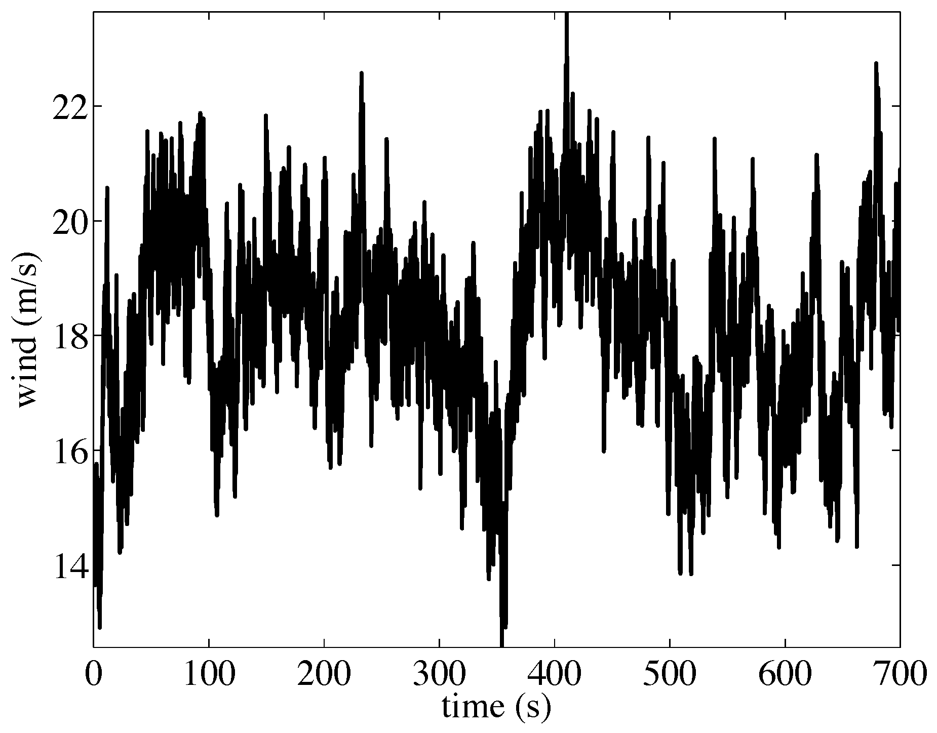
In the simulations, new wind data sets with turbulence intensity set to $10\%$ are generated with TurbSim [22]. It can be seen from Figure 1 that the wind speed covers the full load region, as its values range from $12.91$ m/s up to $22.57$ m/s.

Figure 1. Wind speed signal with turbulence intensity set to $10\%$.

Figure 1. Wind speed signal with turbulence intensity set to $10\%$.

2.2. Generator-Converter Model

The generator-converter system can be approximated by a first-order ordinary differential equation, see [2], which is given by:

$$\dot{{\tau }_r}\left(t\right)+{\alpha }_{gc}{\tau }_r\left(t\right)={\alpha }_{gc}{\tau }_c\left(t\right)$$

(1)

where ${\tau }_r$ and ${\tau }_c$ are the real generator torque and its reference (given by the controller), respectively. In the numerical simulations, ${\alpha }_{gc}=50$, see [21]. Moreover, the power produced by the generator, $P_e\left(t\right)$, is given by (see [2]):

$$P_e\left(t\right)={\eta }_g{\omega }_g\left(t\right){\tau }_r\left(t\right)$$

(2)

where ${\eta }_g$ is the efficiency of the generator and ${\omega }_g$ is the generator speed. In the numerical experiments, ${\eta }_g=0.98$ is used, see [2].

2.3. Pitch Actuator Model

The hydraulic pitch system consists of three identical pitch actuators, which are modeled as a linear differential equation with time-dependent variables, pitch angle $\beta \left(t\right)$ and its reference ${\beta }_r\left(t\right)$. In principle, it is a piston servo-system, which can be expressed as a second-order ordinary differential equation [2]:

$$\ddot{\beta }\left(t\right)+2\xi {\omega }_n\dot{\beta }\left(t\right)+{\omega }_n^2\beta \left(t\right)={\omega }_n^2{\beta }_r\left(t\right)$$

(3)

where ${\omega }_n$ and ξ are the natural frequency and the damping ratio, respectively. For the fault-free case, the parameters $\xi =0.6$ and ${\omega }_n=11.11$ rad/s are used, see [2].

2.4. Fault Scenarios

Both actuator and sensor faults are considered. All the described faults originate from actual faults in wind turbines [2]. Table 2 summarizes all the considered fault scenarios.

Table 2. Fault scenarios.

Number	Fault	Type
F1	Pitch actuator	Change in dynamics: air content in oil
F2	Pitch actuator	Change in dynamics: pump wear
F3	Pitch actuator	Change in dynamics: hydraulic leakage
F4	Torque actuator	Offset
F5	Generator speed sensor	Scaling
F6	Pitch angle sensor	Stuck
F7	Pitch angle sensor	Scaling

Table 2. Fault scenarios.

Number	Fault	Type
F1	Pitch actuator	Change in dynamics: air content in oil
F2	Pitch actuator	Change in dynamics: pump wear
F3	Pitch actuator	Change in dynamics: hydraulic leakage
F4	Torque actuator	Offset
F5	Generator speed sensor	Scaling
F6	Pitch angle sensor	Stuck
F7	Pitch angle sensor	Scaling

2.4.1. Actuator Faults

Pitch actuator faults are studied as they are the actuators with highest failure rate in wind turbines. A fault may change the dynamics of the pitch system by varying the damping ratio $\left(\zeta \right)$ and natural frequencies $\left({\omega }_n\right)$ from their nominal values to their faulty values. The parameters for the pitch system under different conditions are given in Table 3. The normal air content in the hydraulic oil is 7%, whereas the high air content in oil fault (F1) corresponds to 15%. Pump wear (F2) represents the situation of 75% pressure in the pitch system while the parameters stated for hydraulic leakage (F3) correspond to a pressure of only 50%. The three faults are modeled by changing the parameters ${\omega }_n$ and ζ in the relevant pitch actuator model.

Table 3. Change in dynamics pitch actuator faults.

Faults	${\omega }_n$ (rad/s)	ζ
Fault Free(FF)	11.11	0.6
High air content in oil (F1)	5.73	0.45
Pump wear (F2)	7.27	0.75
Hydraulic leakage (F3)	3.42	0.9

Table 3. Change in dynamics pitch actuator faults.

Faults	${\omega }_n$ (rad/s)	ζ
Fault Free(FF)	11.11	0.6
High air content in oil (F1)	5.73	0.45
Pump wear (F2)	7.27	0.75
Hydraulic leakage (F3)	3.42	0.9

For the test, the change in dynamics faults given in Table 3 are introduced only in the third pitch actuator (thus ${\beta }_1$ and ${\beta }_2$ are always fault-free).

A torque actuator fault (F4) is also studied. This fault is an offset on the generated torque, which can be due to an error in the initialization of the converter controller. This fault can occur since the converter torque is estimated based on the currents in the converter. If this estimate is initialized incorrectly it will result in an offset on the estimated converter torque, which leads to the offset on the generator torque. The offset value is 2000 Nm.

2.4.2. Sensor Faults

The generator speed measurement uses encoders and its elements are subject to electrical and mechanical failures, which can result in a changed gain factor on the measurement. The simulated fault, F5, is a gain factor on ${\omega }_g$ equal to 1.2.

Faults 6 and 7 result in blade 3 having a stuck pitch angle sensor, which holds a constant value of $5^{\circ }$ (F6) and ${10}^{\circ }$ (F7), respectively.

Finally, the fault of a gain factor on the measurement of the third pitch angle sensor is studied (F7). The measurement is scaled by a factor of 1.2.

Table 4. Assumed available measurements. These sensors are representative of the types of sensors that are available on a MW-scale commercial wind turbine.

Number	Sensor Type	Symbol	Units
1	Generated electrical power	$P_{e,m}$	kW
2	Rotor speed	${\omega }_{r,m}$	rad/s
3	Generator speed	${\omega }_{g,m}$	rad/s
4	Generator torque	${\tau }_{c,m}$	Nm
5	first pitch angle	${\beta }_{1,m}$	deg
6	second pitch angle	${\beta }_{2,m}$	deg
7	third pitch angle	${\beta }_{3,m}$	deg
8	fore-aft acceleration at tower bottom	$a_{fa,m}^b$	m/s${}^2$
9	side-to-side acceleration at tower bottom	$a_{ss,m}^b$	m/s${}^2$
10	fore-aft acceleration at mid-tower	$a_{fa,m}^m$	m/s${}^2$
11	side-to-side acceleration at mid-tower	$a_{ss,m}^m$	m/s${}^2$
12	fore-aft acceleration at tower top	$a_{fa,m}^t$	m/s${}^2$
13	side-to-side acceleration at tower top	$a_{ss,m}^t$	m/s${}^2$

Table 4. Assumed available measurements. These sensors are representative of the types of sensors that are available on a MW-scale commercial wind turbine.

Number	Sensor Type	Symbol	Units
1	Generated electrical power	$P_{e,m}$	kW
2	Rotor speed	${\omega }_{r,m}$	rad/s
3	Generator speed	${\omega }_{g,m}$	rad/s
4	Generator torque	${\tau }_{c,m}$	Nm
5	first pitch angle	${\beta }_{1,m}$	deg
6	second pitch angle	${\beta }_{2,m}$	deg
7	third pitch angle	${\beta }_{3,m}$	deg
8	fore-aft acceleration at tower bottom	$a_{fa,m}^b$	m/s${}^2$
9	side-to-side acceleration at tower bottom	$a_{ss,m}^b$	m/s${}^2$
10	fore-aft acceleration at mid-tower	$a_{fa,m}^m$	m/s${}^2$
11	side-to-side acceleration at mid-tower	$a_{ss,m}^m$	m/s${}^2$
12	fore-aft acceleration at tower top	$a_{fa,m}^t$	m/s${}^2$
13	side-to-side acceleration at tower top	$a_{ss,m}^t$	m/s${}^2$

3. Fault Detection Strategy

The overall fault detection strategy is based on principal component analysis and statistical hypothesis testing. A baseline pattern or PCA model is created with the healthy state of the wind turbine in the presence of wind turbulence. When the current state of the wind turbine has to be diagnosed, the collected data is projected using the PCA model. The final diagnosis is performed using statistical hypothesis testing.

The main paradigm of vibration based structural health monitoring is based on the basic idea that a change in physical properties due to structural changes or damage will cause detectable changes in dynamical responses. This idea is illustrated in Figure 2, where the healthy structure is excited by a signal to create a pattern. Subsequently, the structure to be diagnosed is excited by the same signal and the dynamic response is compared with the pattern. The scheme in Figure 2 is also know as guided waves in structures for structural health monitoring [23].

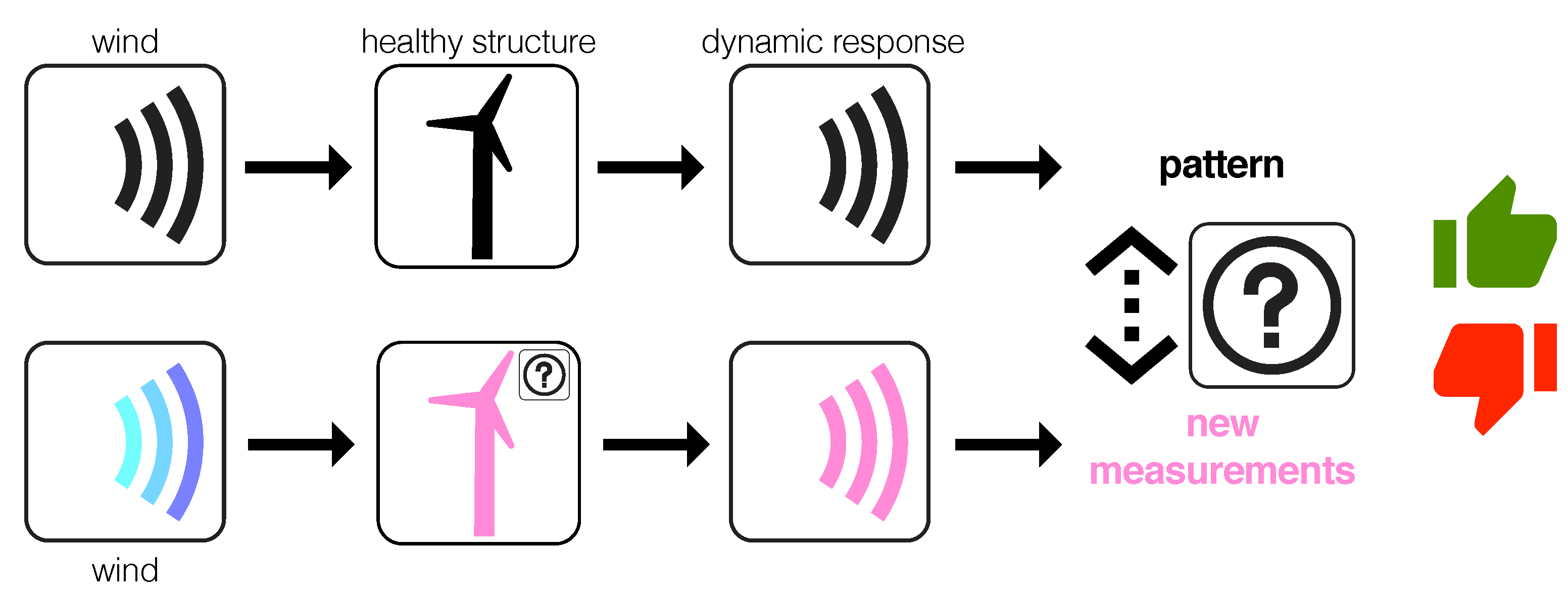
However, in our application, the only available excitation of the wind turbines is the wind turbulence. Therefore, guided waves in wind turbines for SHM as in Figure 2 cannot be considered as a realistic scenario. In spite of that, the new paradigm described in Figure 3 is based on the fact that, even with a different wind turbulence, the fault detection strategy based on PCA and statistical hypothesis testing will be able to detect some damage, fault or misbehavior. More precisely, the key idea behind the detection strategy is the assumption that a change in the behavior of the overall system, even with a different excitation, has to be detected. The results presented in Section 4 confirm this hypothesis.

Figure 2. Guided waves in structures for structural health monitoring. The healthy structure is excited by a signal and the dynamic response is measured to create a baseline pattern. Then, the structure to diagnose is excited by the same signal and the dynamic response is also measured and compared with the baseline pattern. A significant difference in the pattern would imply the existence of a fault.

Figure 2. Guided waves in structures for structural health monitoring. The healthy structure is excited by a signal and the dynamic response is measured to create a baseline pattern. Then, the structure to diagnose is excited by the same signal and the dynamic response is also measured and compared with the baseline pattern. A significant difference in the pattern would imply the existence of a fault.

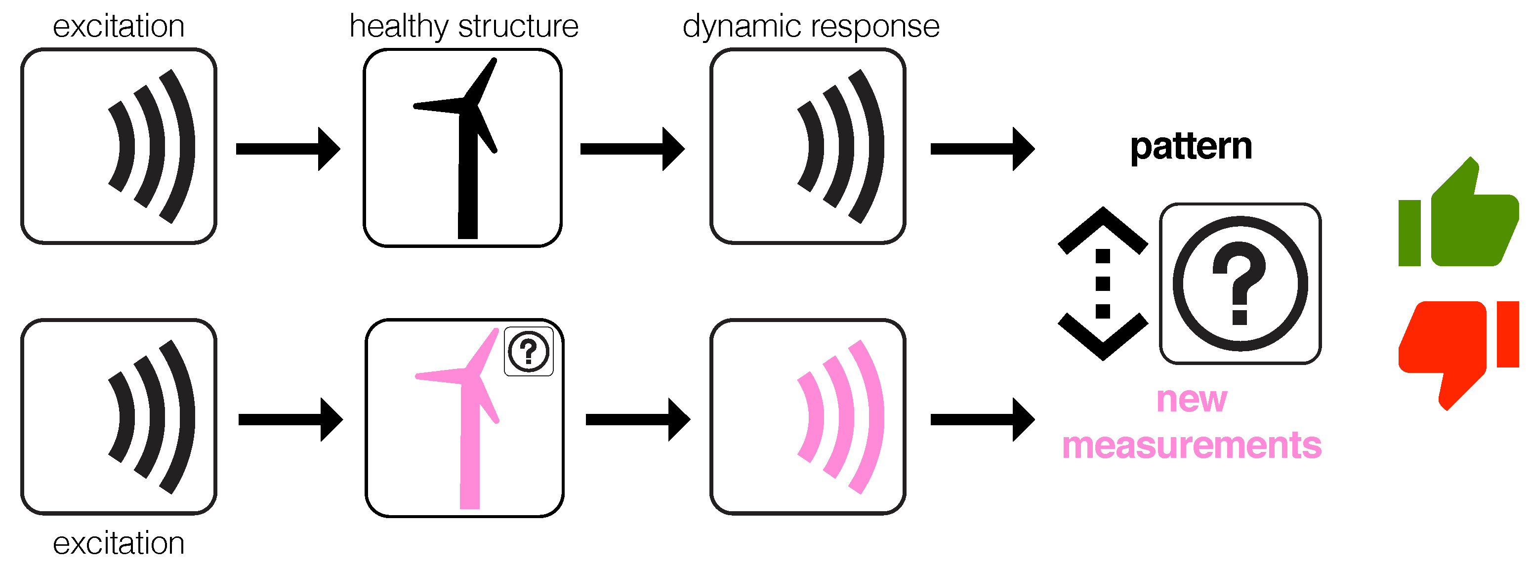
Figure 3. Even with a different wind turbulence, the fault detection strategy is able to detect some damage, fault or misbehavior.

Figure 3. Even with a different wind turbulence, the fault detection strategy is able to detect some damage, fault or misbehavior.

3.1. Data Driven Baseline Modeling Based on PCA

Let us start the PCA modeling by measuring, from a healthy wind turbine, a sensor during $(nL-1)\Delta$ seconds, where Δ is the sampling time and $n,L\in \mathbb{N}$. The discretized measures of the sensor are a real vector

$$\begin{array}{c}\hfill \left(\begin{array}{ccccccccccccc}{x}_{11}& x_{12}& \cdots & x_{1L}& x_{21}& x_{22}& \cdots & x_{2L}& \cdots & x_{n1}& x_{n2}& \cdots & x_{nL}\end{array}\right)\in {\mathbb{R}}^{nL}\end{array}$$

(4)

where the real number $x_{ij},i=1,\dots ,n,j=1,\dots ,L$ corresponds to the measure of the sensor at time $\left((i-1)L+(j-1)\right)\Delta$ seconds. This collected data can be arranged in matrix form as follows:

$$\begin{array}{c}\hfill \left(\begin{array}{cccc}{x}_{11}& x_{12}& \cdots & x_{1L}\\ ⋮& ⋮& \ddots & ⋮\\ x_{i1}& x_{i2}& \cdots & x_{iL}\\ ⋮& ⋮& \ddots & ⋮\\ x_{n1}& x_{n2}& \cdots & x_{nL}\end{array}\right)\in {\mathcal{M}}_{n\times L}\left(\mathbb{R}\right)\end{array}$$

(5)

where ${\mathcal{M}}_{n\times L}\left(\mathbb{R}\right)$ is the vector space of $n\times L$ matrices over $\mathbb{R}$. When the measures are obtained from $N\in \mathbb{N}$ sensors also during $(nL-1)\Delta$ seconds, the collected data, for each sensor, can be arranged in a matrix as in Equation (5). Finally, all the collected data coming from the N sensors is disposed in a matrix $\mathbf{X}\in {\mathcal{M}}_{n\times (N·L)}$ as follows:

$$\begin{array}{cc}\mathbf{X}\hfill & =\left(\begin{array}{cccc}\begin{array}{cccc}{x}_{11}^1& x_{12}^1& \cdots & x_{1L}^1\\ ⋮& ⋮& \ddots & ⋮\\ x_{i1}^1& x_{i2}^1& \cdots & x_{iL}^1\\ ⋮& ⋮& \ddots & ⋮\\ x_{n1}^1& x_{n2}^1& \cdots & x_{nL}^1\end{array}& \begin{array}{ccc}{x}_{11}^2& \cdots & x_{1L}^2\\ ⋮& \ddots & ⋮\\ x_{i1}^2& \cdots & x_{iL}^2\\ ⋮& \ddots & ⋮\\ x_{n1}^2& \cdots & x_{nL}^2\end{array}& \begin{array}{c}\cdots \\ \ddots \\ \cdots \\ \ddots \\ \cdots \end{array}& \begin{array}{ccc}{x}_{11}^N& \cdots & x_{1L}^N\\ ⋮& \ddots & ⋮\\ x_{i1}^N& \cdots & x_{iL}^N\\ ⋮& \ddots & ⋮\\ x_{n1}^N& \cdots & x_{nL}^N\end{array}\end{array}\right)\hfill \\ & =\left(\begin{array}{cccc}{\mathbf{X}}^1& {\mathbf{X}}^2& \cdots & {\mathbf{X}}^N\end{array}\right)\hfill \end{array}$$

(6)

where the superindex $k=1,\dots ,N$ of each element $x_{ij}^k$ in the matrix represents the number of sensor.

The objective of the principal component analysis is to find a linear transformation orthogonal matrix $\mathbf{P}\in {\mathcal{M}}_{(N·L)\times (N·L)}\left(\mathbb{R}\right)$ that will be used to transform or project the original data matrix $\mathbf{X}$ according to the subsequent matrix product:

$$\begin{array}{c}\hfill \mathbf{T}=\mathbf{XP}\in {\mathcal{M}}_{n\times (N·L)}\left(\mathbb{R}\right)\end{array}$$

(7)

where $\mathbf{T}$ is a matrix having a diagonal covariance matrix.

Group Scaling

Since the data in matrix $\mathbf{X}$ is affected by diverse wind turbulence, come from several sensors and could have different scales and magnitudes, it is required to apply a preprocessing step to rescale the data using the mean of all measurements of the sensor at the same column and the standard deviation of all measurements of the sensor [24].

More precisely, for $k=1,2,\dots ,N$ we define

$$\begin{array}{}\mathrm{(8)}& \begin{array}{cc}{\mu }_j^k\hfill & =\frac{1}{n}\sum _{i=1}^n{x}_{ij}^k,j=1,\dots ,L,\hfill \end{array}\mathrm{(9)}& \begin{array}{cc}{\mu }^k\hfill & =\frac{1}{nL}\sum _{i=1}^n\sum _{j=1}^L{x}_{ij}^k,\hfill \end{array}\mathrm{(10)}& \begin{array}{cc}{\sigma }^k\hfill & =\sqrt{\frac{1}{nL}\sum _{i=1}^n\sum _{j=1}^L{(x_{ij}^k-{\mu }^k)}^2}\hfill \end{array}\end{array}$$

where ${\mu }_j^k$ is the mean of the measures placed at the same column, that is, the mean of the n measures of sensor k in matrix ${\mathbf{X}}^k$ at time instants $\left((i-1)L+(j-1)\right)\Delta$ seconds, $i=1,\dots ,n$; ${\mu }^k$ is the mean of all the elements in matrix ${\mathbf{X}}^k$, that is, the mean of all the measures of sensor k; and ${\sigma }^k$ is the standard deviation of all the measures of sensor k. Therefore, the elements $x_{ij}^k$ of matrix $\mathbf{X}$ are scaled to define a new matrix $\check{\mathbf{X}}$ as

$$\begin{array}{cc}\hfill {\check{x}}_{ij}^k& :=\frac{x_{ij}^k-{\mu }_j^k}{{\sigma }^k},i=1,\dots ,n,j=1,\dots ,L,k=1,\dots ,N.\hfill \end{array}$$

(11)

When the data are normalized using Equation (11), the scaling procedure is called variable scaling or group scaling [25].

For the sake of clarity, and throughout the rest of the paper, the scaled matrix $\check{\mathbf{X}}$ is renamed as simply $\mathbf{X}$. The mean of each column vector in the scaled matrix $\mathbf{X}$ can be computed as

$$\begin{array}{}\mathrm{(12)}& \begin{array}{cc}\hfill \frac{1}{n}\sum _{i=1}^n{\check{x}}_{ij}^k& =\frac{1}{n}\sum _{i=1}^n\frac{x_{ij}^k-{\mu }_j^k}{{\sigma }^k}=\frac{1}{n{\sigma }^k}\sum _{i=1}^n\left(x_{ij}^k-{\mu }_j^k\right)\hfill \end{array}\mathrm{(13)}& \begin{array}{cc}& =\frac{1}{n{\sigma }^k}\left[\left(\sum _{i=1}^n{x}_{ij}^k\right)-n{\mu }_j^k\right]\hfill \end{array}\mathrm{(14)}& \begin{array}{cc}& =\frac{1}{n{\sigma }^k}\left(n{\mu }_j^k-n{\mu }_j^k\right)=0\hfill \end{array}\end{array}$$

Since the scaled matrix $\mathbf{X}$ is a mean-centered matrix, it is possible to calculate its covariance matrix as follows:

$${\mathbf{C}}_{\mathbf{X}}=\frac{1}{n-1}{\mathbf{X}}^T\mathbf{X}\in {\mathcal{M}}_{(N·L)\times (N·L)}\left(\mathbb{R}\right)$$

(15)

The covariance matrix ${\mathbf{C}}_{\mathbf{X}}$ is a $(N·L)\times (N·L)$ symmetric matrix that measures the degree of linear relationship within the data set between all possible pairs of columns. At this point it is worth noting that each column can be viewed as a virtual sensor and, therefore, each column vector $\mathbf{X}(:,j)\in {\mathbb{R}}^n,j=1,\dots ,N·L,$ represents a set of measurements from one virtual sensor.

The subspaces in PCA are defined by the eigenvectors and eigenvalues of the covariance matrix as follows:

$${\mathbf{C}}_{\mathbf{X}}\mathbf{P}=\mathbf{P}\Lambda$$

(16)

where the columns of $\mathbf{P}\in {\mathcal{M}}_{(N·L)\times (N·L)}\left(\mathbb{R}\right)$ are the eigenvectors of ${\mathbf{C}}_{\mathbf{X}}$. The diagonal terms of matrix $\Lambda \in {\mathcal{M}}_{(N·L)\times (N·L)}\left(\mathbb{R}\right)$ are the eigenvalues ${\lambda }_i,i=1,\dots ,N·L,$ of ${\mathbf{C}}_{\mathbf{X}}$ whereas the off-diagonal terms are zero, that is,

$$\begin{array}{}\mathrm{(17)}& \begin{array}{cc}\hfill {\Lambda }_{ii}& ={\lambda }_i,i=1,\dots ,N·L\hfill \end{array}\mathrm{(18)}& \begin{array}{cc}\hfill {\Lambda }_{ij}& =0,i,j=1,\dots ,N·L,i\ne j\hfill \end{array}\end{array}$$

The eigenvectors $p_j,j=1,\dots ,N·L$, representing the columns of the transformation matrix $\mathbf{P}$ are classified according to the eigenvalues in descending order and they are called the principal components or the loading vectors of the data set. The eigenvector with the highest eigenvalue, called the first principal component, represents the most important pattern in the data with the largest quantity of information.

Matrix $\mathbf{P}$ is usually called the principal components of the data set or loading matrix and matrix $\mathbf{T}$ is the transformed or projected matrix to the principal component space, also called score matrix. Using all the $N·L$ principal components, that is, in the full dimensional case, the orthogonality of $\mathbf{P}$ implies ${\mathbf{PP}}^{\mathrm{T}}=\mathbf{I}$, where $\mathbf{I}$ is the $(N·L)\times (N·L)$ identity matrix. Therefore, the projection can be inverted to recover the original data as

$$\begin{array}{c}\hfill \mathbf{X}={\mathbf{TP}}^T\end{array}$$

(19)

However, the objective of PCA is, as said before, to reduce the dimensionality of the data set $\mathbf{X}$ by selecting only a limited number $\ell <N·L$ of principal components, that is, only the eigenvectors related to the ℓ highest eigenvalues. Thus, given the reduced matrix

$$\begin{array}{c}\hfill \widehat{\mathbf{P}}=\left(p_1|p_2|\cdots |p_{\ell }\right)\in {\mathcal{M}}_{N·L\times \ell }\left(\mathbb{R}\right)\end{array}$$

(20)

matrix $\widehat{\mathbf{T}}$ is defined as

$$\begin{array}{c}\hfill \widehat{\mathbf{T}}=\mathbf{X}\widehat{\mathbf{P}}\in {\mathcal{M}}_{n\times \ell }\left(\mathbb{R}\right)\end{array}$$

(21)

Note that opposite to $\mathbf{T}$, $\widehat{\mathbf{T}}$ is no longer invertible. Consequently, it is not possible to fully recover $\mathbf{X}$ although $\widehat{\mathbf{T}}$ can be projected back onto the original $N·L-$dimensional space to get a data matrix $\widehat{\mathbf{X}}$ as follows:

$$\begin{array}{c}\hfill \widehat{\mathbf{X}}=\widehat{\mathbf{T}}{\widehat{\mathbf{P}}}^T\in {\mathcal{M}}_{n\times (N·L)}\left(\mathbb{R}\right)\end{array}$$

(22)

The difference between the original data matrix $\mathbf{X}$ and $\widehat{\mathbf{X}}$ is defined as the residual error matrix $\mathbf{E}$ or $\tilde{\mathbf{X}}$ as follows:

$$\begin{array}{c}\hfill \mathbf{E}=\mathbf{X}-\widehat{\mathbf{X}}\end{array}$$

(23)

or, equivalenty,

$$\begin{array}{cc}\hfill \mathbf{X}& =\widehat{\mathbf{X}}+\mathbf{E}=\widehat{\mathbf{T}}{\widehat{\mathbf{P}}}^T+\mathbf{E}\hfill \end{array}$$

(24)

The residual error matrix $\mathbf{E}$ describes the variability not represented by the data matrix $\widehat{\mathbf{X}}$, and can also be expressed as

$$\begin{array}{c}\hfill \mathbf{E}=\mathbf{X}(\mathbf{I}-\widehat{\mathbf{P}}{\widehat{\mathbf{P}}}^T)\end{array}$$

(25)

Even though the real measures obtained from the sensors as a function of time represent physical magnitudes, when these measures are projected and the scores are obtained, these scores no longer represent any physical magnitude [26]. The key aspect in this approach is that the scores from different experiments can be compared with the reference pattern to try to detect a different behavior.

3.2. Fault Detection Based on Hypothesis Testing

The current wind turbine to diagnose is subjected to a wind turbulence as described in Section 2 and Section 3.1. When the measures are obtained from $N\in \mathbb{N}$ sensors during $(\nu L-1)\Delta$ seconds, a new data matrix $\mathbf{Y}$ is constructed as in Equation (6):

$$\begin{array}{cc}\hfill \mathbf{Y}& =\left(\begin{array}{cccc}\begin{array}{cccc}{y}_{11}^1& y_{12}^1& \cdots & y_{1L}^1\\ ⋮& ⋮& \ddots & ⋮\\ y_{i1}^1& y_{i2}^1& \cdots & y_{iL}^1\\ ⋮& ⋮& \ddots & ⋮\\ y_{\nu 1}^1& y_{\nu 2}^1& \cdots & y_{\nu L}^1\end{array}& \begin{array}{ccc}{y}_{11}^2& \cdots & y_{1L}^2\\ ⋮& \ddots & ⋮\\ y_{i1}^2& \cdots & y_{iL}^2\\ ⋮& \ddots & ⋮\\ y_{\nu 1}^2& \cdots & y_{\nu L}^2\end{array}& \begin{array}{c}\cdots \\ \ddots \\ \cdots \\ \ddots \\ \cdots \end{array}& \begin{array}{ccc}{y}_{11}^N& \cdots & y_{1L}^N\\ ⋮& \ddots & ⋮\\ y_{i1}^N& \cdots & y_{iL}^N\\ ⋮& \ddots & ⋮\\ y_{\nu 1}^N& \cdots & y_{\nu L}^N\end{array}\end{array}\right)\in {\mathcal{M}}_{\nu \times (N·L)}\left(\mathbb{R}\right)\hfill \end{array}$$

(26)

It is worth remarking that the natural number ν (the number of rows of matrix $\mathbf{Y}$) is not necessarily equal to n (the number of rows of $\mathbf{X}$), but the number of columns of $\mathbf{Y}$ must agree with that of $\mathbf{X}$; that is, in both cases the number N of sensors and the number of samples per row must be equal.

Before the collected data arranged in matrix $\mathbf{Y}$ is projected into the new space spanned by the eigenvectors in matrix $\mathbf{P}$ in Equation (16), the matrix has to be scaled to define a new matrix $\check{\mathbf{Y}}$ as in Equation (11):

$$\begin{array}{cc}\hfill {\check{y}}_{ij}^k& :=\frac{y_{ij}^k-{\mu }_j^k}{{\sigma }^k},i=1,\dots ,\nu ,j=1,\dots ,L,k=1,\dots ,N,\hfill \end{array}$$

(27)

where ${\mu }_j^k$ and ${\sigma }^k$ are defined in Equations (8) and (10), respectively.

The projection of each row vector $r^i=\check{\mathbf{Y}}(i,:)\in {\mathbb{R}}^{N·L},i=1,\dots ,\nu$ of matrix $\check{\mathbf{Y}}$ into the space spanned by the eigenvectors in $\widehat{\mathbf{P}}$ is performed through the following vector to matrix multiplication:

$$\begin{array}{c}\hfill t^i=r^i·\widehat{\mathbf{P}}\in {\mathbb{R}}^{\ell }\end{array}$$

(28)

For each row vector $r^i,i=1,\dots ,\nu$, the first component of vector $t^i$ is called the first score or score 1; similarly, the second component of vector $t^i$ is called the second score or score 2, and so on.

In a standard application of the principal component analysis strategy in the field of structural health monitoring, the scores allow a visual grouping or separation [27]. In some other cases, as in [28], two classical indices can be used for damage detection, such as the Q index (also known as SPE, square prediction error) and the Hotelling’s $T^2$ index. The Q index of the ith row $y_i^T$ of matrix $\check{\mathbf{Y}}$ is defined as follows:

$$\begin{array}{c}\hfill Q_i=y_i^T(\mathbf{I}-\widehat{\mathbf{P}}{\widehat{\mathbf{P}}}^T)y_i\end{array}$$

(29)

The $T^2$ index of the ith row $y_i^T$ of matrix $\check{\mathbf{Y}}$ is defined as follows:

$$\begin{array}{c}\hfill T_i^2=y_i^T\left(\widehat{\mathbf{P}}{\Lambda }^{-1}{\widehat{\mathbf{P}}}^T\right)y_i\end{array}$$

(30)

In this case, however, it can be observed in Figure 4—where the projection onto the two first principal components of samples coming from the healthy and faulty wind turbines are plotted—that a visual grouping, clustering or separation cannot be performed. A similar conclusion is deducted from Figure 5. In this case, the plot of the natural logarithm of indices Q and $T^2$—defined in Equations (29) and (30)—of samples coming from the healthy and faulty wind turbines does not allow any visual grouping. Therefore, a more powerful and reliable tool is needed to be able to detect a fault in the wind turbine.

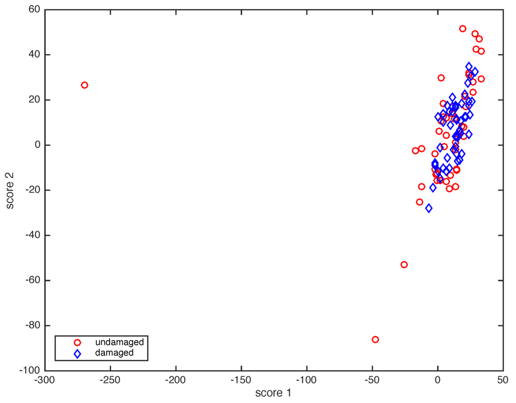
Figure 4. Projection onto the two first principal components of samples coming from the healthy wind turbine (red, circle) and from the faulty wind turbine (blue, diamond).

Figure 4. Projection onto the two first principal components of samples coming from the healthy wind turbine (red, circle) and from the faulty wind turbine (blue, diamond).

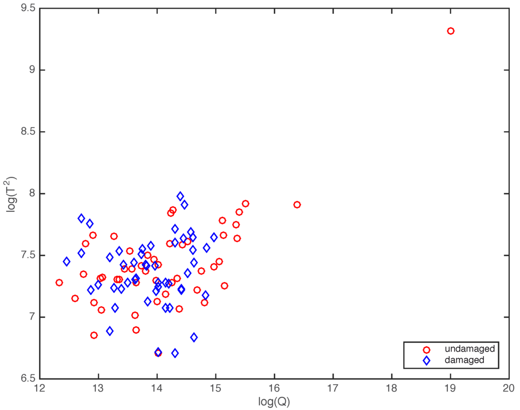
Figure 5. Natural logarithm of indices Q and $T^2$ of samples coming from the healthy wind turbine (red, circle) and from the faulty wind turbine (blue, diamond).

Figure 5. Natural logarithm of indices Q and $T^2$ of samples coming from the healthy wind turbine (red, circle) and from the faulty wind turbine (blue, diamond).

3.2.1. The Random Nature of the Scores

Since the turbulent wind can be considered as a random process, the dynamic response of the wind turbine can be considered as a stochastic process and the measurements in $r^i$ are also stochastic. Therefore, each component of $t^i$ acquires this stochastic nature and it will be regarded as a random variable to construct the stochastic approach in this paper.

3.2.2. Test for the Equality of Means

The objective of the present work is to examine whether the current wind turbine is healthy or subjected to a fault as those described in Table 2. To achieve this end, we have a PCA model (matrix $\widehat{\mathbf{P}}$ in Equation (20)) built as in Section 3.1.1 with data coming from a wind turbine in a full healthy state. For each principal component $j=1,\dots ,\ell$, the baseline sample is defined as the set of n real numbers computed as the $j-$th component of the vector to matrix multiplication $\mathbf{X}(i,:)·\widehat{\mathbf{P}}$. Note that n is the number of rows of matrix $\mathbf{X}$ in Equation (6). That is, we define the baseline sample as the set of numbers ${\left\{{\tau }_j^i\right\}}_{i=1,\dots ,n}$ given by

$$\begin{array}{c}\hfill {\tau }_j^i:=(\mathbf{X}(i,:)·\widehat{\mathbf{P}})\left(j\right)=\mathbf{X}(i,:)·\widehat{\mathbf{P}}·{\mathbf{e}}_j,i=1,\dots ,n,\end{array}$$

(31)

where ${\mathbf{e}}_j$ is the $j-$th vector of the canonical basis.

Similarly, and for each principal component $j=1,\dots ,\ell$, the sample of the current wind turbine to diagnose is defined as the set of ν real numbers computed as the $j-$th component of the vector $t^i$ in Equation (28). Note that ν is the number of rows of matrix $\mathbf{Y}$ in Equation (26). That is, we define the sample to diagnose as the set of numbers ${\left\{t_j^i\right\}}_{i=1,\dots ,\nu }$ given by

$$\begin{array}{c}\hfill t_j^i:=t^i·{\mathbf{e}}_j,i=1,\dots ,\nu .\end{array}$$

(32)

As said before, the goal of this paper is to obtain a fault detection method such that when the distribution of the current sample is related to the distribution of the baseline sample a healthy state is predicted and otherwise a fault is detected. To that end, a test for the equality of means will be performed. Let us consider that, for a given principal component, (a) the baseline sample is a random sample of a random variable having a normal distribution with unknown mean ${\mu }_X$ and unknown standard deviation ${\sigma }_X$; and (b) the random sample of the current wind turbine is also normally distributed with unknown mean ${\mu }_Y$ and unknown standard deviation ${\sigma }_Y$. Let us finally consider that the variances of these two samples are not necessarily equal. As said previously, the problem that we will consider is to determine whether these means are equal, that is, ${\mu }_X={\mu }_Y$, or equivalently, ${\mu }_X-{\mu }_Y=0$. This statement leads immediately to a test of the hypotheses

$$\begin{array}{}\mathrm{(33)}& \begin{array}{cc}{H}_0:\hfill & {\mu }_X-{\mu }_Y=0\text{versus}\hfill \end{array}\mathrm{(34)}& \begin{array}{cc}{H}_1:\hfill & {\mu }_X-{\mu }_Y\ne 0\hfill \end{array}\end{array}$$

that is, the null hypothesis is “the sample of the wind turbine to be diagnosed is distributed as the baseline sample” and the alternative hypothesis is “the sample of the wind turbine to be diagnosed is not distributed as the baseline sample”. In other words, if the result of the test is that the null hypothesis is not rejected, the current wind turbine is categorized as healthy. Otherwise, if the null hypothesis is rejected in favor of the alternative, this would indicate the presence of some faults in the wind turbine.

The test is based on the Welch-Satterthwaite method [29], which is outlined below. When random samples of size n and ν, respectively, are taken from two normal distributions $N\left({\mu }_X,{\sigma }_X\right)$ and $N\left({\mu }_Y,{\sigma }_Y\right)$ and the population variances are unknown, the random variable

$$\begin{array}{c}\hfill \mathcal{W}=\frac{\left(\overline{X}-\overline{Y}\right)+({\mu }_X-{\mu }_Y)}{\sqrt{\left({\displaystyle \frac{S_X^2}{n}}+{\displaystyle \frac{S_Y^2}{\nu }}\right)}}\end{array}$$

(35)

can be approximated with a t-distribution with ρ degrees of freedom, that is

$$\begin{array}{c}\hfill \mathcal{W}\hookrightarrow t_{\rho }\end{array}$$

(36)

where

$$\begin{array}{c}\hfill \rho =⌊{\displaystyle \frac{{\left({\displaystyle \frac{s_X^2}{n}}+{\displaystyle \frac{s_Y^2}{\nu }}\right)}^2}{{\displaystyle \frac{{(s_X^2/n)}^2}{n-1}}+{\displaystyle \frac{{(s_Y^2/\nu )}^2}{\nu -1}}}}⌋\end{array}$$

(37)

and where $\overline{X},\overline{Y}$ is the sample mean as a random variable; $S^2$ is the sample variance as a random variable; $s^2$ is the variance of a sample; and $\lfloor ·\rfloor$ is the floor function.

The value of the standardized test statistic using this method is defined as

$$\begin{array}{c}\hfill t_{\mathrm{obs}}={\displaystyle \frac{\overline{x}-\overline{y}}{\sqrt{\left({\displaystyle \frac{s_X^2}{n}}+{\displaystyle \frac{s_Y^2}{\nu }}\right)}}}\end{array}$$

(38)

where $\overline{x},\overline{y}$ is the mean of a particular sample. The quantity $t_{\mathrm{obs}}$ is the fault indicator. We can then construct the following test:

$$\begin{array}{}\mathrm{(39)}& \begin{array}{cc}\left|t_{\mathrm{obs}}\right|\le t^{\star }\hfill & ⟹\text{Fail}\text{to}\text{reject}{H}_0\hfill \end{array}\mathrm{(40)}& \begin{array}{cc}\left|t_{\mathrm{obs}}\right|>t^{\star }\hfill & ⟹\text{Reject}{H}_0\hfill \end{array}\end{array}$$

where $t^{\star }$ is such that

$$\begin{array}{c}\hfill P\left(t_{\rho }<t^{\star }\right)=1-\frac{\alpha }{2}\end{array}$$

(41)

and α is the chosen risk (significance) level for the test. More precisely, the null hypothesis is rejected if $\left|t_{\mathrm{obs}}\right|>t^{\star }$ (this would indicate the existence of a fault in the wind turbine). Otherwise, if $\left|t_{\mathrm{obs}}\right|\le t^{\star }$ there is no statistical evidence to suggest that both samples are normally distributed but with different means, thus indicating that no fault in the wind turbine has been found. This idea is represented in Figure 6.

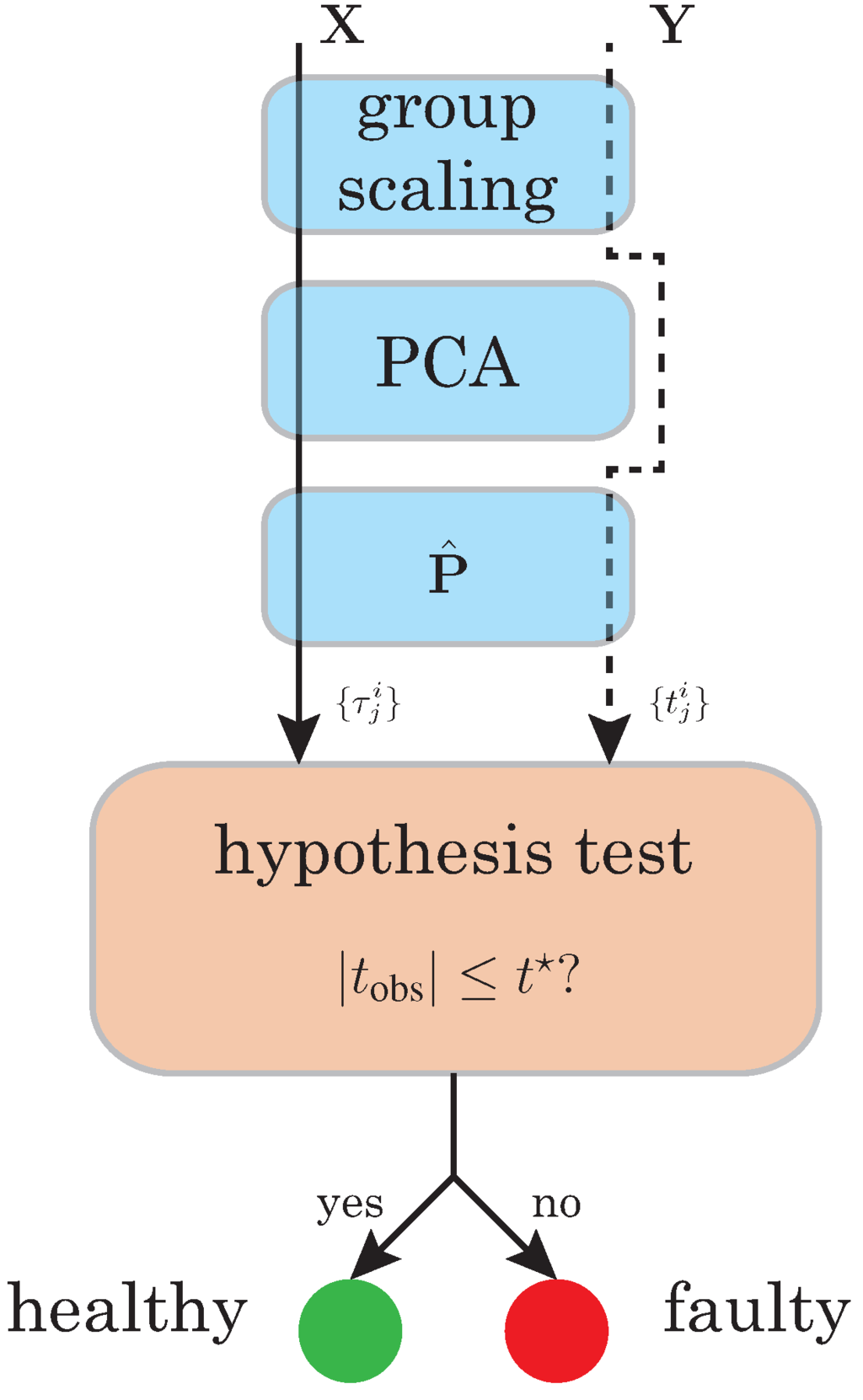
Figure 6. Fault detection will be based on testing for significant changes in the distributions of the baseline sample and the sample coming from the wind turbine to diagnose.

Figure 6. Fault detection will be based on testing for significant changes in the distributions of the baseline sample and the sample coming from the wind turbine to diagnose.

4. Simulation Results

4.1. Type I and Type II errors

To validate the fault detection strategy presented in Section 3, we first consider a total of 24 samples of $\nu =50$ elements each, according to the following distribution:

• 16 samples of a healthy wind turbine; and
• 8 samples of a faulty wind turbine with respect to each of the eight different fault scenarios described in Table 2.

In the numerical simulations in this Section, each sample of $\nu =50$ elements is composed by the measures obtained from the $N=13$ sensors detailed in Table 4 during $(\nu ·L-1)\Delta =312.4875$ seconds, where $L=500$ and the sampling time $\Delta =0.0125$ seconds. The measures of each sample are then arranged in a $\nu \times (N·L)$ matrix as in Equation (26).

For the first four principal components (score 1 to score 4), these 24 samples plus the baseline sample of $n=50$ elements are used to test for the equality of means, with a level of significance $\alpha =0.36$ (the choice of this level of significance will be justified in Section 4.2). Each sample of $\nu =50$ elements is categorized as follows: (i) number of samples from the healthy wind turbine (healthy sample) which were classified by the hypothesis test as “healthy” (fail to reject $H_0$); (ii) faulty sample classified by the test as “faulty” (reject $H_0$); (iii) samples from the faulty structure (faulty sample) classified as “healthy”; and (iv) faulty sample classified as “faulty”. The results for the first four principal components presented in Table 6 are organized according to the scheme in Table 5. It can be stressed from each principal component in Table 6 that the sum of the columns is constant: 16 samples in the first column (healthy wind turbine) and 8 more samples in the second column (faulty wind turbine).

Table 5. Scheme for the presentation of the results in Table 6.

	Undamaged Sample ($H_0$)	Damaged Sample ($H_1$)
Fail to reject $H_0$	Correct decision	Type II error (missing fault)
Reject $H_0$	Type I error (false alarm)	Correct decision

Table 5. Scheme for the presentation of the results in Table 6.

	Undamaged Sample ($H_0$)	Damaged Sample ($H_1$)
Fail to reject $H_0$	Correct decision	Type II error (missing fault)
Reject $H_0$	Type I error (false alarm)	Correct decision

Table 6. Categorization of the samples with respect to the presence or absence of damage and the result of the test for each of the four scores when the size of the samples to diagnose is $\nu =50$.

	score 1			score 2			score 3			score 4
	$H_0$	$H_1$		$H_0$	$H_1$		$H_0$	$H_1$		$H_0$	$H_1$
Fail to reject $H_0$	16	0		12	1		11	5		9	1
Reject $H_0$	0	8		4	7		5	3		7	7

Table 6. Categorization of the samples with respect to the presence or absence of damage and the result of the test for each of the four scores when the size of the samples to diagnose is $\nu =50$.

	score 1			score 2			score 3			score 4
	$H_0$	$H_1$		$H_0$	$H_1$		$H_0$	$H_1$		$H_0$	$H_1$
Fail to reject $H_0$	16	0		12	1		11	5		9	1
Reject $H_0$	0	8		4	7		5	3		7	7

In Table 6, it is worth noting that two kinds of misclassification are presented which are denoted as follows:

• Type I error (false positive or false alarm), when the wind turbine is healthy but the null hypothesis is rejected and therefore classified as faulty. The probability of committing a type I error is α, the level of significance.
• Type II error (false negative or missing fault), when the structure is faulty but the null hypothesis is not rejected and therefore classified as healthy. The probability of committing a type II error is called γ.

It can be observed from Table 6 that, in the numerical simulations, Type I errors (false alarms) and Type II errors (missing faults) appear only when scores 2, 3 or 4 are considered, while when the first score is used all the decisions are correct. The better performance of the first score is an expected result in the sense that the first principal component is the component that accounts for the largest possible variance.

4.2. Sensitivity and Specificity

Two more statistical measures can be selected here to study the performance of the test: the sensitivity and the specificity. The sensitivity, also called as the power of the test, is defined, in the context of this work, as the proportion of samples from the faulty wind turbine which are correctly identified as such. Thus, the sensitivity can be computed as $1-\gamma$. The specificity of the test is defined, also in this context, as the proportion of samples from the healthy structure that are correctly identified and can be expressed as $1-\alpha$.

The sensitivity and the specificity of the test with respect to the 24 samples and for each of the first four principal components –organized as shown in Table 7– have been included in Table 8.

Table 7. Relationship between type I and type II errors.

	Undamaged Sample ($H_0$)	Damaged Sample ($H_1$)
Fail to reject $H_0$	Specificity ($1-\alpha$)	False negative rate (γ)
Reject $H_0$	False positive rate (α)	Sensitivity ($1-\gamma$)

Table 7. Relationship between type I and type II errors.

	Undamaged Sample ($H_0$)	Damaged Sample ($H_1$)
Fail to reject $H_0$	Specificity ($1-\alpha$)	False negative rate (γ)
Reject $H_0$	False positive rate (α)	Sensitivity ($1-\gamma$)

Table 8. Sensitivity and specificity of the test for each of the four scores when the size of the samples to diagnose is $\nu =50$.

	score 1			score 2			score 3			score 4
	$H_0$	$H_1$		$H_0$	$H_1$		$H_0$	$H_1$		$H_0$	$H_1$
Fail to reject $H_0$	1.00	0.00		0.75	0.13		0.69	0.62		0.56	0.13
Reject $H_0$	0.00	1.00		0.25	0.87		0.31	0.38		0.44	0.87

Table 8. Sensitivity and specificity of the test for each of the four scores when the size of the samples to diagnose is $\nu =50$.

	score 1			score 2			score 3			score 4
	$H_0$	$H_1$		$H_0$	$H_1$		$H_0$	$H_1$		$H_0$	$H_1$
Fail to reject $H_0$	1.00	0.00		0.75	0.13		0.69	0.62		0.56	0.13
Reject $H_0$	0.00	1.00		0.25	0.87		0.31	0.38		0.44	0.87

It is worth mentioning that type I errors are frequently considered to be more serious than type II errors. However, in this application, a type II error is related to a missing fault whereas a type I error is related to a false alarm. In consequence, type II errors should be reduced. Therefore a small level of significance of $1\%$, $5\%$ or even $10\%$ would lead to a reduced number of false alarms but to a higher rate of missing faults. That is the reason of the choice of a level of significance of $36\%$ in the hypothesis test.

The results in Table 8 show that the sensitivity of the test $1-\gamma$ is close to $100\%$, as desired, with an average value of $78.00\%$. The sensitivity with respect to the first, second and fourth principal component is increased, in mean, to a $91.33\%$. The average value of the specificity is $75.00\%$, which is very close to the expected value of $1-\alpha =64\%$.

4.3. Reliability of the Results

Using the scheme in Table 9, the results are computed and given in Table 10. This table is based on the Bayes’ theorem [30], where P($H_1|\mathrm{accept}{H}_0$) is the proportion of samples from the faulty wind turbine that have been incorrectly classified as healthy (true rate of false negatives) and P($H_0|\mathrm{accept}{H}_1$) is the proportion of samples from the healthy wind turbine that have been incorrectly classified as faulty (true rate of false positives).

Table 9. Relationship between the proportion of false negatives and false positives.

	Undamaged Sample ($H_0$)	Damaged Sample ($H_1$)
Fail to reject $H_0$	P($H_0|\mathrm{accept}{H}_0$)	$\begin{array}{c}\mathrm{true}\mathrm{rate}\mathrm{of}\mathrm{false}\mathrm{negatives}\hfill \\ P\left(H_1\right|\mathrm{accept}{H}_0)\hfill \end{array}$
Reject $H_0$	$\begin{array}{c}\mathrm{true}\mathrm{rate}\mathrm{of}\mathrm{false}\mathrm{positives}\hfill \\ P\left(H_0\right|\mathrm{accept}{H}_1)\hfill \end{array}$	P($H_1|\mathrm{accept}{H}_1$)

Table 9. Relationship between the proportion of false negatives and false positives.

	Undamaged Sample ($H_0$)	Damaged Sample ($H_1$)
Fail to reject $H_0$	P($H_0|\mathrm{accept}{H}_0$)	$\begin{array}{c}\mathrm{true}\mathrm{rate}\mathrm{of}\mathrm{false}\mathrm{negatives}\hfill \\ P\left(H_1\right|\mathrm{accept}{H}_0)\hfill \end{array}$
Reject $H_0$	$\begin{array}{c}\mathrm{true}\mathrm{rate}\mathrm{of}\mathrm{false}\mathrm{positives}\hfill \\ P\left(H_0\right|\mathrm{accept}{H}_1)\hfill \end{array}$	P($H_1|\mathrm{accept}{H}_1$)

Table 10. True rate of false positives and false negatives for each of the four scores when the size of the samples to diagnose is $\nu =50$.

	score 1			score 2			score 3			score 4
	$H_0$	$H_1$		$H_0$	$H_1$		$H_0$	$H_1$		$H_0$	$H_1$
Fail to reject $H_0$	1.00	0.00		0.92	0.08		0.69	0.31		0.90	0.10
Reject $H_0$	0.00	1.00		0.36	0.64		0.62	0.38		0.50	0.50

Table 10. True rate of false positives and false negatives for each of the four scores when the size of the samples to diagnose is $\nu =50$.

	score 1			score 2			score 3			score 4
	$H_0$	$H_1$		$H_0$	$H_1$		$H_0$	$H_1$		$H_0$	$H_1$
Fail to reject $H_0$	1.00	0.00		0.92	0.08		0.69	0.31		0.90	0.10
Reject $H_0$	0.00	1.00		0.36	0.64		0.62	0.38		0.50	0.50

4.4. The Receiver Operating Curves (ROC)

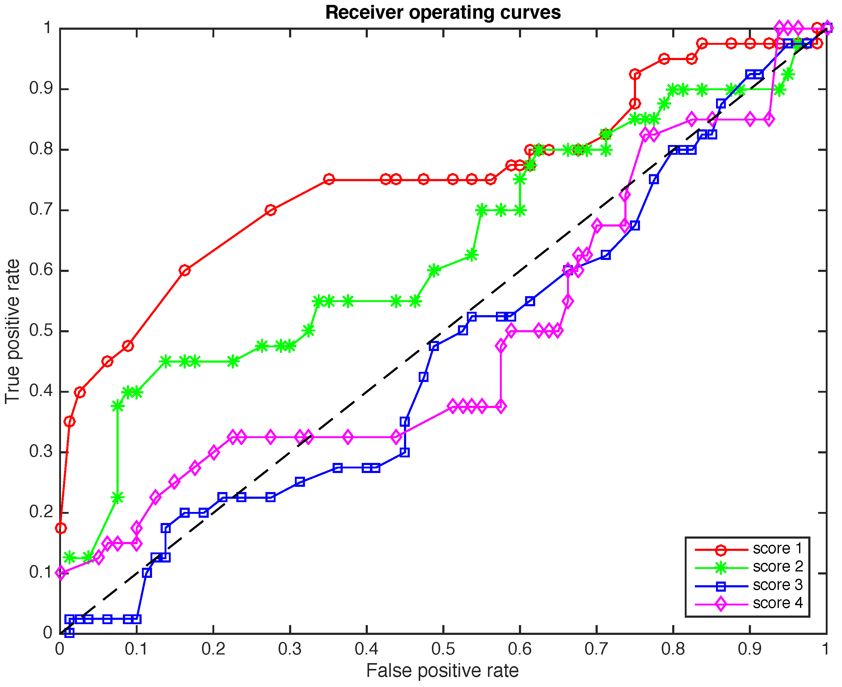
An additional study has been developed based on the ROC curves to determine the overall accuracy of the proposed method. These curves represent the trade-off between the false positive rate and the sensitivity in Table 10 for different values of the level of significance that is used in the statistical hypothesis testing. Note that the false positive rate is defined as the complementary of the specificity, and therefore these curves can also be used to visualize the close relationship between specificity and sensitivity. It can also be remarked that the sensitivity is also called true positive rate or probability of detection [31]. More precisely, for each principal component and for a given level of significance the pair of numbers

$$\begin{array}{c}\hfill \left(\text{false positive rate, sensitivity}\right)\in [0,1]\times [0,1]\subset {\mathbb{R}}^2\end{array}$$

(42)

is plotted. We have considered 49 levels of significance within the range $[0.02,0.98]$ and with a difference of $0.02$. Therefore, for each of the first four principal components, 49 connected points are depicted, as can be seen in Figure 7.

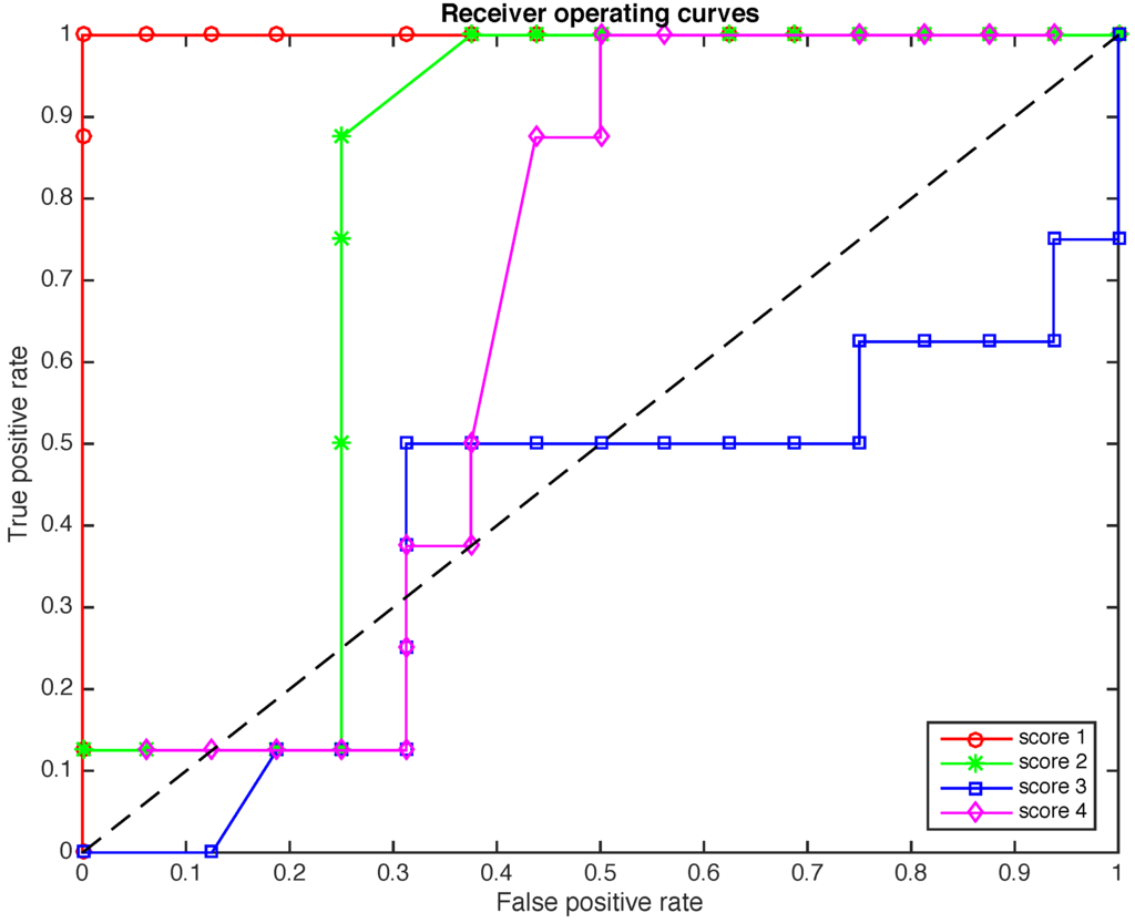
Figure 7. The Receiver Operating Curves (ROCs) for the four scores when the size of the samples to diagnose is $\nu =50$.

Figure 7. The Receiver Operating Curves (ROCs) for the four scores when the size of the samples to diagnose is $\nu =50$.

The placement of these points can be interpreted as follows. Since we are interested in reducing the number of false positives while we increase the number of true positives, these points must be placed in the upper-left corner as much as possible. However, this is not always possible because there is also a relationship between the level of significance and the false positive rate. Therefore, a method can be considered acceptable if those points lie within the upper-left half-plane. In this sense, the results presented in Figure 7, particularly with respect to score 1, are quite remarkable. The overall behavior of scores 2 and 4 are also acceptable, while the results of score 3 cannot be considered, in this case, as satisfactory.

In Figure 8 and Figure 9 a further study is performed. While in Figure 7 we present the ROCs when the size of the samples to diagnose is $\nu =50$, in Figure 8 the reliability of the method is analyzed in terms of 48 samples of $\nu =25$ elements each and in Figure 9 the reliability of the method is analyzed in terms of 120 samples of $\nu =10$ elements each. The effect of reducing the number of elements in each sample is the reduction in the total time needed for a diagnostic. More precisely, if we keep $L=500$, when the size of the samples is reduced from $\nu =50$ to $\nu =25$ and $\nu =10$, the total time needed for a diagnostic is reduced from about 312 s to 156 and 62 s, respectively. Another effect of the reduction in the number of elements in each sample is a slight deterioration of the overall accuracy of the detection method. However, the results of scores 1 and 2 in Figure 8 and Figure 9 are perfectly acceptable.

A very interesting alternative to keep a very good performance of the method without almost no degradation in its accuracy is by reducing L –the number of time instants per row per sensor— instead of reducing the number of elements per sample ν. This way, if we keep $\nu =50$, when L is reduced from 500 to 50, the total time needed for a diagnostic is reduced from about 312 s to 31 s.

We can finally say that the ROC curves provide a statistical assessment of the efficacy of a method and can be used to visualize and compare the performance of multiple scenarios.

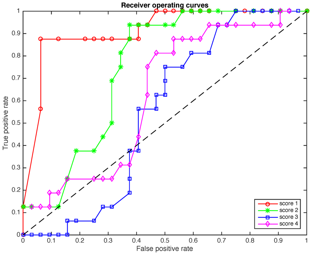
Figure 8. The ROCs for the four scores when the size of the samples to diagnose is $\nu =25$.

Figure 8. The ROCs for the four scores when the size of the samples to diagnose is $\nu =25$.

Figure 9. The ROCs for the four scores when the size of the samples to diagnose is $\nu =10$.

Figure 9. The ROCs for the four scores when the size of the samples to diagnose is $\nu =10$.

5. Conclusions

The silver bullet for offshore operators is to eliminate unscheduled maintenance. Therefore, the implementation of fault detection systems is crucial. The main challenges of the wind turbine fault detection lie in its nonlinearity, unknown disturbances as well as significant measurement noise. In this work, numerical simulations (with a well-known benchmark wind turbine) show that the proposed PCA plus statistical hypothesis testing is a valuable tool in fault detection for wind turbines. It is noteworthy that, in the simulations, when the first score is used all the decisions are correct (there are no false alarms and no missing faults).

We believe that PCA plus statistical hypothesis testing has tremendous potential in decreasing maintenance costs. Therefore, we view the work described in this paper as only the beginning of a large project. For future work, we plan to develop a complete fault detection, isolation, and reconfiguration method (FDIR). That is, a reconfigurable control strategy in response to faults. In the near future, the next step is to focus our research into efficient fault feature extraction.

References

- Sinha, Y.; Steel, J. A progressive study into offshore wind farm maintenance optimisation using risk based failure analysis. Renew. Sustain. Energy Rev. 2015, 42, 735–742. [Google Scholar] [CrossRef]
- Odgaard, P.; Johnson, K. Wind turbine fault diagnosis and fault tolerant control—An enhanced benchmark challenge. In Proceedings of the 2013 American Control Conference (ACC), Washington, DC, USA, 17–19 June 2013; pp. 1–6.
- Soman, R.N.; Malinowski, P.H.; Ostachowicz, W.M. Bi-axial neutral axis tracking for damage detection in wind-turbine towers. Wind Energy 2015. [Google Scholar] [CrossRef]
- Adams, D.; White, J.; Rumsey, M.; Farrar, C. Structural health monitoring of wind turbines: Method and application to a HAWT. Wind Energy 2011, 14, 603–623. [Google Scholar] [CrossRef]
- Griffith, D.T.; Yoder, N.C.; Resor, B.; White, J.; Paquette, J. Structural health and prognostics management for the enhancement of offshore wind turbine operations and maintenance strategies. Wind Energy 2014, 17, 1737–1751. [Google Scholar] [CrossRef]
- Ding, S.X. Model-Based Fault Diagnosis Techniques: Design Schemes, Algorithms, and Tools; Springer Science & Business Media: London, UK, 2008. [Google Scholar]
- Odgaard, P.F.; Stoustrup, J.; Nielsen, R.; Damgaard, C. Observer based detection of sensor faults in wind turbines. In Proceedings of the European Wind Energy Conference, Marseille, France, 16–19 March 2009; pp. 4421–4430.
- Zhang, X.; Zhang, Q.; Zhao, S.; Ferrari, R.M.; Polycarpou, M.M.; Parisini, T. Fault detection and isolation of the wind turbine benchmark: An estimation-based approach. In Proceedings of the International Federation of Automatic Control (IFAC) World Congress, Milano, Italy, 28 August–2 September 2011; Volume 2, pp. 8295–8300.
- Shaker, M.S.; Patton, R.J. Active sensor fault tolerant output feedback tracking control for wind turbine systems via T-S model. Eng. Appl. Artif. Intell. 2014, 34, 1–12. [Google Scholar] [CrossRef]
- Shi, F.; Patton, R. An active fault tolerant control approach to an offshore wind turbine model. Renew. Energy 2015, 75, 788–798. [Google Scholar] [CrossRef]
- Vidal, Y.; Tutiven, C.; Rodellar, J.; Acho, L. Fault diagnosis and fault-tolerant control of wind turbines via a discrete time controller with a disturbance compensator. Energies 2015, 8, 4300–4316. [Google Scholar] [CrossRef]
- Dong, J.; Verhaegen, M. Data driven fault detection and isolation of a wind turbine benchmark. In Proceedings of the International Federation of Automatic Control (IFAC) World Congress, Milano, Italy, 28 August–2 September 2011; Volume 2, pp. 7086–7091.
- Simani, S.; Castaldi, P.; Tilli, A. Data-driven approach for wind turbine actuator and sensor fault detection and isolation. In Proceedings of the International Federation of Automatic Control (IFAC) World Congress, Milano, Italy, 28 August–2 September 2011; pp. 8301–8306.
- Laouti, N.; Sheibat-Othman, N.; Othman, S. Support vector machines for fault detection in wind turbines. In Proceedings of International Federation of Automatic Control (IFAC) World Congress, Milano, Italy, 28 August–2 September 2011; Volume 2, pp. 7067–7072.
- Stoican, F.; Raduinea, C.F.; Olaru, S. Adaptation of set theoretic methods to the fault detection of wind turbine benchmark. In Proceedings of the International Federation of Automatic Control (IFAC) World Congress, Milano, Italy, 28 August–2 September 2011; pp. 8322–8327.
- Odgaard, P.F.; Stoustrup, J. Gear-box fault detection using time-frequency based methods. Annu. Rev. Control 2015, 40, 50–58. [Google Scholar] [CrossRef]
- Pang-Ning, T.; Steinbach, M.; Kumar, V. Introduction to Data Mining; Pearson Addison Wesley: Boston, MA, USA, 2005. [Google Scholar]
- Zaher, A.; McArthur, S.; Infield, D.; Patel, Y. Online wind turbine fault detection through automated SCADA data analysis. Wind Energy 2009, 12, 574. [Google Scholar] [CrossRef]
- Kusiak, A.; Li, W.; Song, Z. Dynamic control of wind turbines. Renew. Energy 2010, 35, 456–463. [Google Scholar] [CrossRef]
- Jonkman, J. NWTC Information Portal (FAST). Available online: https://nwtc.nrel.gov/FAST (accessed on 18 December 2015).
- Jonkman, J.M.; Butterfield, S.; Musial, W.; Scott, G. Definition of a 5-MW Reference Wind Turbine for Offshore System Development; National Renewable Energy Laboratory: Golden, CO, USA, 2009. [Google Scholar]
- Kelley, N.; Jonkman, B. NWTC Information Portal (Turbsim). Available online: https://nwtc.nrel.gov/TurbSim (accessed on 18 December 2015).
- Ostachowicz, W.; Kudela, P.; Krawczuk, M.; Zak, A. Guided Waves in Structures for SHM: The Time-Domain Spectral Element Method; John Wiley & Sons, Ltd: Hoboken, NJ, USA, 2012. [Google Scholar]
- Anaya, M.; Tibaduiza, D.; Pozo, F. A bioinspired methodology based on an artificial immune system for damage detection in structural health monitoring. Shock Vibration 2015, 2015, 1–15. [Google Scholar] [CrossRef]
- Anaya, M.; Tibaduiza, D.; Pozo, F. Detection and classification of structural changes using artificial immune systems and fuzzy clustering. Int. J. Bio-Inspired Comput. in press.
- Mujica, L.E.; Ruiz, M.; Pozo, F.; Rodellar, J.; Güemes, A. A structural damage detection indicator based on principal component analysis and statistical hypothesis testing. Smart Mater. Struct. 2014, 23, 1–12. [Google Scholar] [CrossRef]
- Mujica, L.E.; Rodellar, J.; Fernández, A.; Güemes, A. Q-statistic and T2-statistic PCA-based measures for damage assessment in structures. Struct. Health Monit. 2011, 10, 539–553. [Google Scholar] [CrossRef]
- Odgaard, P.F.; Lin, B.; Jorgensen, S.B. Observer and data-driven-model-based fault detection in power plant coal mills. IEEE Trans. Energy Convers. 2008, 23, 659–668. [Google Scholar] [CrossRef]
- Ugarte, M.D.; Militino, A.F.; Arnholt, A. Probability and Statistics with R; Chemical Rubber Company (CRC) Press: Boca Raton, FL, USA, 2008. [Google Scholar]
- De Groot, M.H.; Schervish, M.J. Probability and Statistics; Pearson: Boston, MA, USA, 2012. [Google Scholar]
- Yinghui, L.; Michaels, J.E. Feature extraction and sensor fusion for ultrasonic structural health monitoring under changing environmental conditions. IEEE Sens. J. 2009, 9, 1462–1471. [Google Scholar] [CrossRef]
© 2015 by the authors; licensee MDPI, Basel, Switzerland. This article is an open access article distributed under the terms and conditions of the Creative Commons by Attribution (CC-BY) license (http://creativecommons.org/licenses/by/4.0/).