In this section we introduce the proposed EMS framework by discussing its architecture and internals.
4.2. The ICT Infrastructure
The ICT infrastructure has been designed to pursue a set of goals:
the field devices should work independently from the EMS in case of no provided input;
the infrastructure should be flexible enough to accustom multiple adapters comprising a wide range of field devices;
the data collection rate from field devices is independent of the EMS decisions and depends on the specific field device;
the EMS takes its decisions evaluating system state snapshots at a given time and available forecasts regarding future energy production/consumption of generators/loads;
the EMS chooses one energy production/consumption pattern for each generator/load: the pattern includes power consumption set points for each involved field device within a given time horizon. Field actuators are in charge of translating set points into commands to be issued to devices;
the EMS running frequency and optimization horizon might change over time.
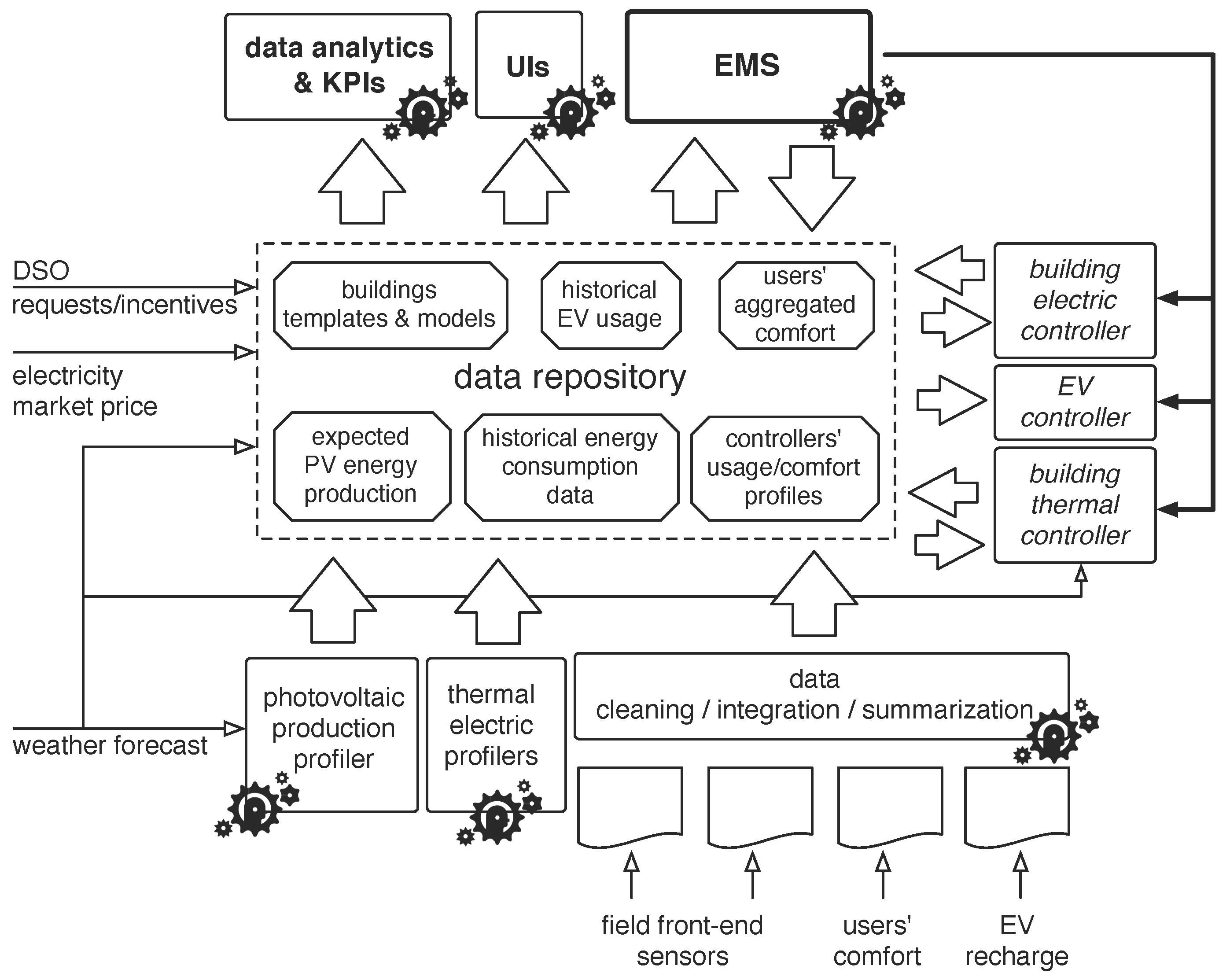
On the basis of the stated goals, the ICT infrastructure leverages the two main functional elements in the back-end: the data repository and the EMS. The data repository collects data from the field gateways (which read the field sensors), from the forecast models, and from the EMS (which logs its decisions). Data is available to the EMS, profilers, business intelligence processes and data presentation applications.
The EMS is designed to run at every time slot, but it can be configured to run with a different frequency (e.g., a lower one). The EMS collects the information needed for the optimization from the data repository and executes the optimization algorithm. The optimization output consists of power demand scheduling for passive loads, such as HVACs and EVs, and of storage scheduling for power generated by RESes.
In general, the EMS bases its decisions on predictions which field devices cannot always adhere to. For example, the energy production generated by PV units or power demanded by EVs can be lower than expected. For this reason, the EMS pushes field devices schedules to a group of controllers that transform set points into constraints on the maximum power that each device is allowed to drain from/inject into the system. Prediction errors are prevented in two ways: small errors are handled by running the EMS frequently and by using up-to-date data at each iteration. The EMS continuously updates its decisions to cope with changing conditions and to avoid large accumulated errors, thus limiting inefficiencies. Large errors, such as a completely wrong weather forecast, are dealt by each controller, which can raise the EMS constraints if the controlled field device cannot provide its minimum service. This happens, for example, with the HVACs: when the allocated power results in a too low (or too high) temperature and, consequently, in a too high users’ discomfort, the controller could remove the constraint thus allowing the system to work freely.
The back-end domain comprises the data repository, the EMS and a set of forecast models. The data repository can be hosted either within campus data centers or at any Infrastructure/Platform as a Service (IaaS/PaaS) provider. Back-end components interact with external data sources such as the DSO or the weather forecast service using the Internet, and with the data presentation applications and field front-end by means of the campus LAN.
Gateways and controllers are physical devices equipped with a networking interface, thus enabling communication with sensors and actuators and with the back-end module. Moreover, they are supplied with sufficient computational capabilities to fulfill some predefined automated control operations, such as lifting power constraints if target values can not be met by sensors. Generally, controllers also behave as gateways and interact with the back-end domain.
4.3. The Data Repository
The EMS is able to take educated decisions based on the available information collected during the lifetime of the system and stored in the so-called
data repository, depicted in
Figure 2. In order not to overload the repository with too many data which are not of interest except for the data provider (which would see the repository as a local database) or for the single actor (that would use the repository as a data exchange mean), only information exploited by more than two (sub)systems is stored and shared. In particular, the following pieces of information are stored:
electricity market prices, collected daily;
data collected from sensors monitoring the building thermal conditions, energy consumption (within the buildings and from the EV chargers) and the users’ feedback on their thermal comfort, collected with a tunable frequency;
weather forecasts used to support the estimation of PV energy production as well as the expected energy consumption to heat/cool the building spaces, collected daily;
EV recharge information, collected dynamically;
photovoltaic sources energy production, collected dynamically;
accepted DRE manifests;
energy consumption/production profiles selected by the EMS at each time-slot, providing the on-going strategy actuated by the EMS, collected every time the EMS takes a decision;
models and technical details for all the elements constituting the system (e.g., building/offices structural information, sensors and actuators datasheets ...).
As discussed, these data are used by the EMS to make decisions based on the historical behavior of the system and of the users (e.g., past energy consumption patterns) and on the forecasts of the future demands. In this case, data can be collected with the appropriate frequency (e.g., weather conditions are monitored every 30 min) and periodically pushed to the data repository, since it is not exploited in real-time by any actor, including the EMS. Indeed, there are situations where real-time interaction is needed between two actors (e.g., the EMS and the EV recharge station to interrupt the action in order to immediately reduce energy consumption) and thus direct communication is supported and only the result of the activity is then stored in the data repository.
As a consequence, data in the repository constitutes the system status, updated with a variable delay in the range of tens of minutes. They constitute the source for user applications (such as the one for providing the user comfort feedback), data audit and analysis (also with diagnostic aims), and public displays.
Since data is produced by different (and sometimes redundant) sources, data are integrated, cleaned and summarized, in order to be exploited by the EMS and other controllers. More in detail, a three-layer architecture has been designed for the data repository with the aim of providing a flexible and extensible framework, possibly dealing with different application environments and integrating commercial as well as proprietary data collection solutions.
The lower layer collects raw data from the field (
i.e., from wired/wireless sensors, EV recharge stations and energy production/consumption monitors). Gateways have been used to decouple data collection from transmission to the data repository, adopting a polling-based acquisition approach, to manage the high (and possibly variable) number of sensors. This level has been implemented using a NoSQL datastore, Cassandra [
28], a distributed database management system designed to handle large amounts of semi-structured heterogeneous data and providing high availability and fault tolerance. A set of distributed algorithms to perform data cleaning and summarization have also been implemented. Furthermore, the system provides online data analysis using an SQL-like query language and supports batch processing over its distributed file system, thus enabling additional
data analytics and
KPI evaluations to improve the EMS mission.
The middle layer of the architecture has been implemented with a relational database in PostgreSQL; it is used to store the processed raw data. Data coming from the electricity market, the weather forecast, and DRE manifests are directly stored in this middle layer. As mentioned, together with the dynamic data coming from the various sources, the data repository also stores all the static structured data on the (sub)systems and components characteristics.
The EMS and other controllers/actors access this data through the top layer, which consists in a set of REST APIs, for a coherent access to the information.
4.4. The EMS Interaction Protocol
The core of the EMS is the Optimizer,
i.e., an algorithm which chooses the power usage profile of each electric actor that allows the system to minimize the cost function. We now list the parameters taken as input by the Optimizer, which are summarized in
Table 1.
Let
and
be the set of power loads and generation plants, respectively. Each plant
is associated to an economic incentive
which is remitted to the EMS for each unit of produced energy. Every electric subsystem (either load or generation plant) is managed by a Profile Generator (PG). Each PG comprises a prediction model of the managed subsystem and is capable of generating several feasible consumption/production profiles. The Optimizer and the PGs operate over a finite scheduling horizon partitioned in a set
of time slots of configurable duration (e.g., for a large campus environment, we consider 15-minute time slots, whereas for a private detached house we consider 5-min intervals). The Optimizer is scheduled to run at the beginning of each time slot and interacts with the other entities according to the protocol in
Figure 3.
First, the Optimizer obtains the time-varying energy prices over the optimization horizon. The prices can be provided by the utility, fetched from the day-ahead market exchange, or predicted in case of participation to the real-time market. At the same time, the Optimizer obtains the list of active DREs. Let
be the set of DRE manifests the EMS may adhere to. Such requests are associated to a set of time slots
indicating the request validity time window and to an economic incentive
which is remitted to the EMS upon acceptance. The requests are categorized in four subsets:
: set of requests d to limit the power absorption below the threshold value for each time slot ;
: set of requests d to maintain the power absorption above the threshold value for each time slot ;
: set of requests d to limit the power injection below the threshold value for each time slot ;
: set of requests d to maintain the power injection above the threshold value for each time slot ;
It follows that . Note that the sets are defined over non-overlapping time windows, i.e., each time slot is included in the validity time span of at most one request. In case no requests are available during a time slot, the maximum amount of injected/absorbed energy is limited by the contractual thresholds .
Then, the Optimizer queries the PG of the uncontrollable power loads and generators. These include e.g., lights, elevators, computing equipment, and power sources without energy storage devices. Each of these PGs provides a prediction of the expected energy consumption or generation in each time slot of the optimization horizon.
If the optimization window includes any time slot which falls in a DRE specifying an upper bound for the absorbed power, the Optimizer calculates, for those time slots, the controllable power limit that can be absorbed from the grid by subtracting the uncontrollable power consumption and adding the uncontrollable power generation. Then, the Optimizer executes an algorithm for splitting the controllable power limit into a power limit mask for each PG managing a controllable load (i.e., a manageable appliance whose consumption can be deferred, interrupted and/or tuned). In our implementation, each PG is associated with a predefined weight and the Optimizer simply splits the limit according to these weights. The Optimizer employs a similar algorithm to calculate a power limit mask for PGs managing controllable sources if the optimization windows contains DREs specifying an upper bound to the injected power.
Next, the Optimizer sends to each controllable PG the power limit mask and queries for a set of profiles over the optimization horizon. Each PG must propose one or more feasible profiles corresponding to different comfort levels and different energy consumption or generation schedules. In case the EMS advertises a power limit, then the PGs should also propose profiles that satisfy the limit in addition to the usual profiles, so that the EMS can decide whether to comply to the DRE requests. The strategy used to elaborate the proposal is PG-specific and depends on the available field data and available models. In general, each PG should be able to provide at least one backup profile, which might be suboptimal.
The separation between Optimizer and PGs makes it possible to cope with time-varying, non-linear constraints without jeopardizing the manageability of the linear optimization model. For example a storage system might have constraints with respect to the number of daily charge/discharge cycles. This can be easily implemented in the PG for the storage system, which proposes only solutions with a duty cycle compatible with the expected battery aging. In turn, the optimizer is bound to choose one of the proposed profiles.
Each power load (generation plant) is then characterized by a set of power consumption/production profiles
(
). Note that the optimization algorithm of the EMS is agnostic w.r.t. the criteria the profile generation process is based on. Such criteria may take into account several factors such as the weather forecasts, the trend of the electricity prices, and the users’ preferences. Each generated profile comprises:
a unique ID;
a list of set points and their corresponding time schedule to enforce the system to behave according to the profile shape;
a 24-h profile (), indicating the expected average power consumption or generation for each time slot ;
a 24-h profile of the expected comfort for each time slot (this profile may represent thermal comfort, or the satisfaction of the users of the electric vehicles: the exact semantic depends on the specific PG); a threshold on the minimum comfort level that each load must ensure for every time slot is also included.
a gain or cost () associated to the profile, which may take into account the usage of non-electric power sources such as gas for heating, the exploitation of economic incentives for using RESes, or different wear and tear costs. Gains are expressed with negative values, whereas costs are expressed with positive values.
Once all the queried PGs provide their list, the Optimizer chooses the best combination of profiles by means of the algorithm described in
Section 4.5 and sends the chosen profile ID back to each PG. Each PG is then responsible of enforcing the chosen profile by configuring the relevant controllers so that the field devices behave as desired.
It is worth noting that controllers are configured for an entire optimization horizon, but the configuration can be overwritten at each optimization time slot if external conditions change, (e.g., better predictions are available or new DRE is published by the DSO).


 ,
, 


