Abstract
To reveal the effect of high-temperature creep on the blade-tip radial running clearance of aeroengine high-pressure turbines, a distributed collaborative generalized regression extremum neural network is proposed by absorbing the heuristic thoughts of distributed collaborative response surface method and the generalized extremum neural network, in order to improve the reliability analysis of blade-tip clearance with creep behavior in terms of modeling precision and simulation efficiency. In this method, the generalized extremum neural network was used to handle the transients by simplifying the response process as one extremum and to address the strong nonlinearity by means of its nonlinear mapping ability. The distributed collaborative response surface method was applied to handle multi-object multi-discipline analysis, by decomposing one “big” model with hyperparameters and high nonlinearity into a series of “small” sub-models with few parameters and low nonlinearity. Based on the developed method, the blade-tip clearance reliability analysis of an aeroengine high-pressure turbine was performed subject to the creep behaviors of structural materials, by considering the randomness of influencing parameters such as gas temperature, rotational speed, material parameters, convective heat transfer coefficient, and so forth. It was found that the reliability degree of the clearance is 0.9909 when the allowable value is 2.2 mm, and the creep deformation of the clearance presents a normal distribution with a mean of 1.9829 mm and a standard deviation of 0.07539 mm. Based on a comparison of the methods, it is demonstrated that the proposed method requires a computing time of 1.201 s and has a computational accuracy of 99.929% over 104 simulations, which are improvements of 70.5% and 1.23%, respectively, relative to the distributed collaborative response surface method. Meanwhile, the high efficiency and high precision of the presented approach become more obvious with the increasing simulations. The efforts of this study provide a promising approach to improve the dynamic reliability analysis of complex structures.
1. Introduction
Creep is induced by the excessive plastic deformation of high-temperature components in an aeroengine, and seriously influences the performance of blade-tip radial running clearance (BTRRC) and aeroengine. Therefore, effectively designing and controlling the BTRRC is significant in the development of high-performance and high-reliability aeroengines [1]. Under aeroengine operation, the BTRRC is variable, with its work status being subject to numerous loads such as heat load, mechanical load, aerodynamic load, and so forth; therefore, the methods and technology of reasonable BTRRC design were the principal concern of [2,3,4]. Most early works on BTRRC design focused on deterministic analysis by adopting the margin method to ensure the safety of the blade tip [3,4]. Unfortunately, this method ignores randomness and uncertainty of impact factors on the BTRRC, such that it is difficult to reflect the actual change rule of the BTRRC. In fact, most impact parameters, such as geometric sizes, material parameters, physical loads, and so on, inherently hold some randomness and uncertainty during fabrication and operation. With respect to the BTRRC, one alternative approach for deterministic analysis is the probabilistic method, which takes account of the randomness of design parameters. Therefore, it is urgent to conduct reliability analysis of BTRRC with respect to the randomness of parameters from a probabilistic perspective, in order to acquire more practical results catering to engineering.
With the development of probabilistic design in structural reliability [5,6,7,8,9], numerous approaches have appeared, mainly consisting of direct simulation methods combined with the Monte Carlo (MC) method [10,11] and the surrogate model approach (also called response surface method, RSM) [12,13]. Although the MC method has high simulation precision in structural reliability analysis subject to precise finite element (FE) models, practical loads, and boundary conditions, the computational efficiency of the MC method finds it difficult to meet the requirements of probabilistic analysis of complex structures with excessive computational burdens due to their complex structure and conditions, such as variable geometry, high nonlinearity, transients, endured loads, and so forth [9]. To address this issue, the surrogate model method, especially quadratic polynomial-based RSM, was developed to improve the efficiency of the probabilistic analysis of complex structures, finding widespread application in many engineering fields [12,13]. However, the RSM is unsatisfying with respect to computing precision due to the approximation of quadratic polynomials to real models. With the development of reliability theory and computer technology, advanced response surface methods have emerged through the integration of advanced algorithms [14,15]. Zhang et al. [16] developed an extremum response surface method (ERSM) in order to overcome the transient problem in the dynamic reliability analysis of flexible mechanisms and validated the ERSM to be highly computationally efficient with acceptable precision. Lu et al. [17] developed an improved ERSM for the reliability sensitivity analysis of multi-failure compressor blisk, by introducing a Kriging model into the ERSM model. The dynamic analysis of BTRRC involves many objects (i.e., disk, blade, casing), multiple disciplines (thermodynamics, aerodynamics, rotodynamics, etc.), transients (time-varying characteristics), hyperparameters (large-scale design variables) and a high degree of nonlinearity. This analysis is a multi-object multi-discipline (MOMD) transient nonlinear analysis with hyperparameters, whereby the computational burden is greatly increased. Therefore, it is difficult to directly adopt the above RSMs for the BTRRC reliability analysis. To address this issue, Bai and Fei [18,19] proposed a distributed collaborative response surface method (DCRSM) to carry out the reliability analysis of an aeroengine high-pressure BTRRC, and illustrated the validity of DCRSM in efficiency and accuracy. Later, to further improve the DCRSM in BTRRC reliability design and turbine blisk reliability evaluation, Fei et al. [20] developed a distributed collaborative extremum response surface method (DCERSM) by incorporating the ERSM concept to handle the transient analytical problem. The investigation in [18,19,20] demonstrated that the DCRSM has potential in MOMD probabilistic analysis with high modeling precision and simulation efficiency, providing useful insights for the purpose of improving the current BTRRC reliability analysis in this paper.
With the development of artificial intelligence, the presence of generalized regression neural network (GRNN) [21] opens the possibility for further enhancing the DCRSM with respect to computing precision and efficiency, because the GRNN has strong nonlinear mapping ability and robustness and small samples, and thus can address highly nonlinear problems, reduce the extraction of samples, and improve the modeling speed. Adel et al. [22] established the GRNN model to predict the wastage of condensers and verified the accuracy of the developed GRNN model. Zhao et al. [23] built the widely used GRNN model to predict the quantity of shipments based on small samples. Machado et al. [24] adopted GRNN to optimize the wavelet transform of voltage signals in electrical power system. Li et al. [25] combined the fruit fly optimization algorithm and GRNN to structure the prediction model of power load. Zhang et al. [26] discussed generalized regression extremum neural network (GRENN) model based on GRNN and ERSM in order to improve the analytical precision of an aeroengine turbine blisk fatigue life reliability analysis. Sun et al. [27] revealed that GRNN had a short training time, good stability and high fitting precision by comparing it to a back propagation neural network for the prediction of air quality. All of the above works show the merits of GRNN with respect to computational accuracy and efficiency.
To improve the computational efficiency and precision of BTRRC dynamic reliability analysis with many objects, multiple disciplines, high nonlinearity, transients, and hyperparameters, this paper proposes distributed collaborative generalized regression extreme neural network (DCGRENN) method, by incorporating both the highly nonlinear mapping ability of ERSM and the MOMD coordination potential of DCRSM. In the DCGRENN, the GRENN is used to handle the transient problem by simplifying the response process as one extremum value and address the nonlinearity by the nonlinear mapping capacity. The thought of DCRSM is applied to handle MOMD analysis with hyperparameters and high nonlinearity by decomposing the “big” model into a series of “small” sub-models with few parameters and low nonlinearity. The DCGRENN is employed in order to carry out the reliability analysis of turbine BTRRC subject to the creep behaviors of structural materials by considering the randomness of influencing parameters. In addition, the comparison of methods is conducted to validate the DCGRENN.
The remainder of this paper is organized as follows. The theory and method of DCGRENN are discussed in Section 2, comprising high-temperature creep theory, GRNN, GRENN, DCGRENN and reliability calculation approaches. Section 3 investigates the dynamic reliability analysis of turbine BTRRC with DCGRENN method, including the flowchart of BTRRC reliability analysis with DCGRENN, the finite element (FE) analysis of BTRRC, DCGRENN modeling, BTRRC reliability analysis with DCGRENN and DCGRENN validation. In Section 4, the main conclusions are summarized.
2. Theory and Methods
2.1. High-Temperature Creep Theory
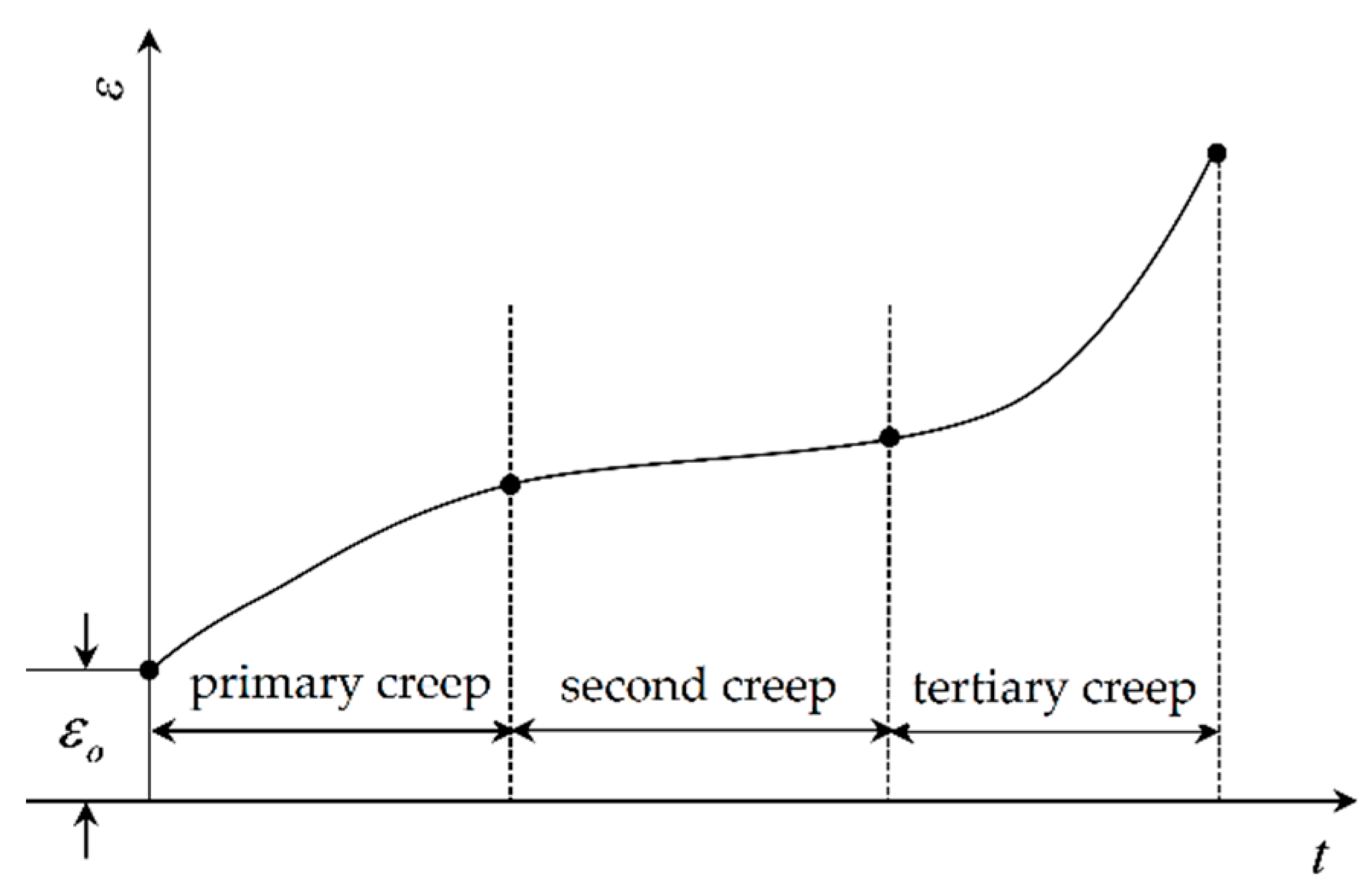
In mechanical strength, the creep of a structure is the permanent deformation of aeroengine turbine structures induced by high temperature load when the stress is less than yield strength [28]. Obviously, creep curve describes the variation of the strain ε of structural materials with time t, as explained in Figure 1.
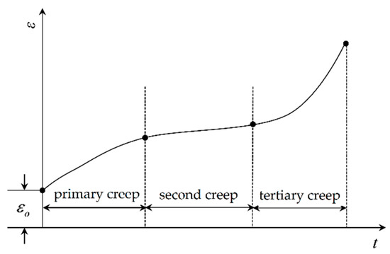
Figure 1.
Creep curve of a structure.
In engineering, the Norton implicit model is usually adopted to express the second constitutive relation of structural materials [29], i.e.,
in which is creep strain; Ci (i = 1, 2, 3) is the parameter of material creep; T is test temperature.
Based on the creep tensile experiment of the material GH4133B (Ni-Cr-based precipitation hardening-type deformation high-temperature alloy) under cyclic loading, the creep data are obtained. Based on the least squares method [30], the creep parameters of GH4133B were obtained and are presented in Table 1.

Table 1.
The creep parameters of GH4133B material.
With respect to the obtained creep parameters (C1, C2 and C3), the creep model of GH4133Bis built as presented in Equation (1), and this will be used in the calculation of blade-tip clearance in the investigation below, regarding GH4133B as the material of the BTRRC.
2.2. Generalized Regression Neural Network
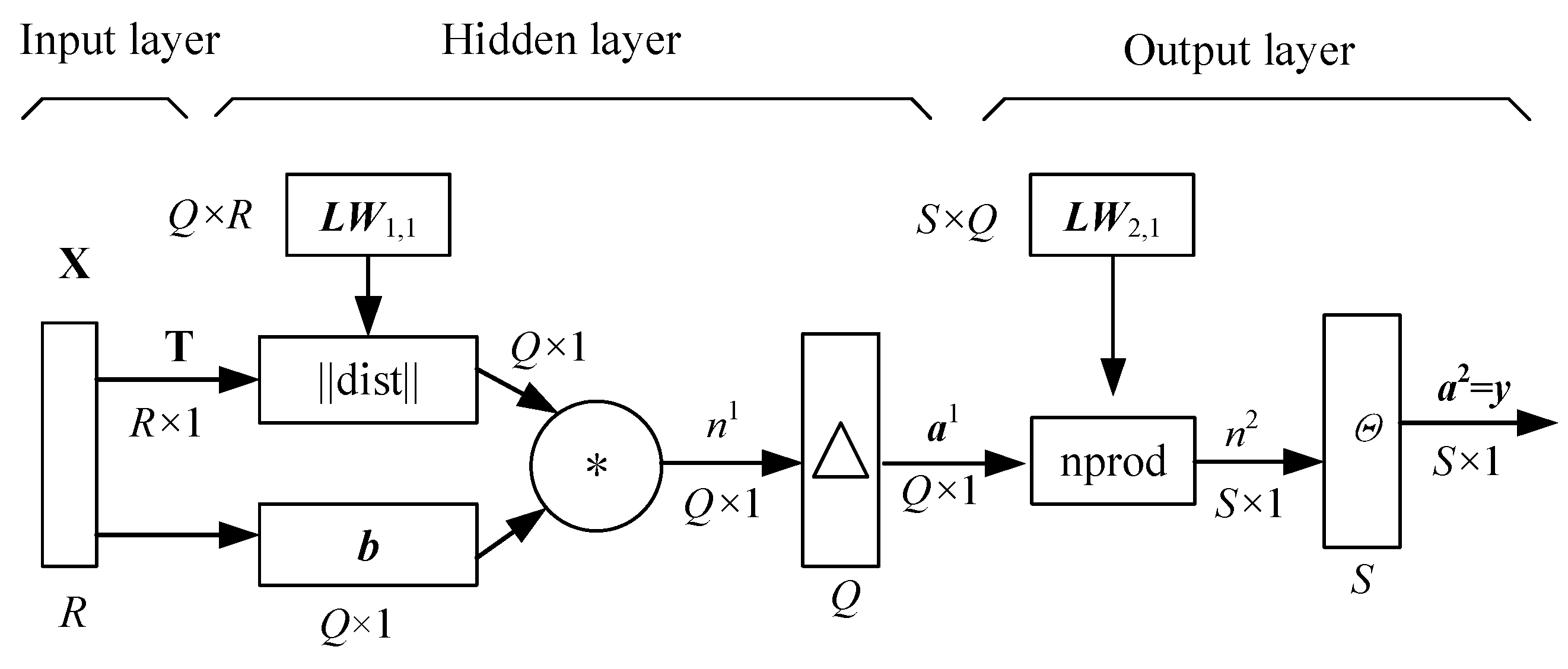
The generalized regression neural network (GRNN) is a nonlinear regression-based feedforward neural network model, including an input layer, a hidden layer, and an output layer [26]. The GRNN has good ability for nonlinear mapping and achieves satisfactory precision between input parameters and output response when carrying out nonlinear modeling. The network structure of GRNN is illustrated in Figure 2.

Figure 2.
The schematic diagram of the generalized regression neural network.
In Figure 2, X and T are the matrices of input samples and output samples, respectively; Q × R indicates the dimensions of matrix LW1,1, which is the weighted matrix in the hidden layer, where Q and R are the numbers of training samples and input parameters, respectively; ||dist|| denotes the Euclidean distance function; b is the threshold of Q neural cells in the hidden layer; n1 expresses the network vector of the hidden layer; △ indicates the transfer (Gauss) function; a1 is the output of the neuro cell; S × Q indicates the dimensions of the matrix LW2,1, which is the connection threshold value between the hidden layer and the output layer, where S is the number of output parameters; nprod is the weight function of the output layer; n2 indicates the network vector of output layer; Θ is the purelin transfer function of the output layer; y = a2 explains the outputs of the neuro cell in the output layer. The input layer transmits the sample X into the hidden layer, in which one nerve cell has one sample and there are Q nerve cells. In the process of transmission, the transfer function is a Gauss function with the matrix of weights and the threshold level vector b. The third layer is the output layer to which the information is transferred from the hidden layer with respect to the matrix of weights LW2,1. Herein, the weight function is the normalized dot product function denoted by nprod.
With respect to the line transfer function of the jth output nj of the GRNN model, the mathematical model of GRNN for the response of the jth group of training samples is expressed by
where exp is the natural exponential function; indicates the output vector of Q nerve cells corresponding to the jth group of input samples, in which (i = 1, 2, …, Q) is the ith element in .
2.3. Generalized Regression Extremum Neural Network Method
Since dynamic probabilistic analysis is a random process, it is difficult to resolve the probabilistic analysis of complex structures by directly adopting the GRNN method. In this case, the traditional approaches involve fitting a large number of response surface models in the time domain, and then artificially selecting the response at one time point as the probabilistic computing point [20]. However, it is hard for this method to guarantee the precision of the selected computing point in engineering applications. To overcome this issue, a generalized regression extremum neural network (GRENN) method is developed by introducing the thought of extremum response into the GRNN model. The GRENN method simplifies the dynamic output response of numerous response models based on the GRNN method as one extremum value of the response process. In this paper, the maximum output responses of input samples in time domain [0, T] are focused on dynamic probabilistic analysis. The basic concept behind the GRENN method is explained in Figure 3.
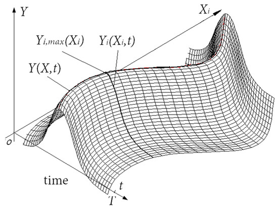
Figure 3.
The basic concept of the generalized regression extremum neural network method.
In Figure 3, () is the output response of the ith input sample in the time domain [0,T] and is the maximum of () in the time domain. When denotes the set comprising the maximum output responses corresponding to all input samples, the fitted extremum response curve is obtained, as follows:
where Q is the number of samples.
Based on the mathematical model of GRNN in Equation (2), the mathematical model of GRENN is
in which i indicates the ith training sample; j expresses the ith random variable.
2.4. Distributed Collaborative Generalized Regression Extremum Neural Network
Although the GRENN method holds promise with respect to solving the transient problem in structural dynamic probabilistic analysis, it still poses one challenge in handling the dynamic probabilistic analysis of structural systems involving multiple objects, multiple disciplines, and hyperparameters. If the GRENN is directly applied to the probabilistic analysis of MOMD structure, it is unworkable for effectively dealing with the analysis problem of many objects and multiple disciplines simultaneously. To address this issue, the DCGRENN method is developed by integrating the thoughts of DCRSM [18] and GRENN [26]. Distributed coordinative technique in DCRSM is applied to handle the MOMD analysis by dividing the “big” model with high-nonlinearity and hyperparameters into a series of simple “small” models with low nonlinearity and few parameters. GRENN is used to address the transient problem in dynamic probabilistic analysis by reducing the response process as one extreme value, and to deal with the problem of nonlinearity by through its ability in highly nonlinear mapping. In other words, in MOMD dynamic probabilistic analysis using the DCGRENN method, the whole (“big”) model of the MOMD structure is divided into many single-object single-discipline (SOSD) sub-models (“small” models), so that the probabilistic analysis of the “big” MOMD model is decomposed into a large number of “small” SOSD models. In the process of SOSD probabilistic analysis, the GRENN models of SOSD models are built as distributed GRENNs (DGRENNs). We consider the responses of DGRENN models as the inputs for the collaborative generalized regression extreme neural network (CGRENN) method in order to perform a collaborative dynamic probabilistic analysis of the structure. The collaborative relationship among the extremum outputs of sub-models is addressed for MOMD dynamic probabilistic analysis. Therefore, the distributed collaborative strategy with GRENN is likely to overcome the problem of MOMD analysis, transient response and hyperparameters in the dynamic probabilistic analysis of complex structures, and then to improve the analytical precision and efficiency.
When one mechanical structure comprises m (m∈Z) objects (substructures) and the analysis of each object involves n (n∈Z) disciplines, with respect to the DC strategy, the complicated MOMD analysis is transferred into a series of simple SOSD analyses. When X(pq) is the input sample vector of qth discipline in pth object, the corresponding output response, Y(pq) is expressed as
subject to
where k is the number of random variables in single discipline.
According to Equation (4), the DGRENN model is defined as
in which and are the weight matrix in the hidden layer, weight matrix in the output layer and the output vector of the output layer in the DGRENN model of disciplines.
Regarding the output responses of the qth discipline in the pth object as the random input variables of the pth object model analysis, i.e.,
When is the response of the pth object, the response surface function (DGRENN) of objects is
Here, , and are the weight matrix in the hidden layer, weight matrix in the output layer and the output vector of the output layer in the DGRENN model of objects.
Similarly, regarding the outputs of all of the object analyses as the random input variables of the whole coordinative model (CGRENN), i.e.,
the output response of the MOMD overall CGRENN model is
where , and are the weight matrix in the hidden layer, weight matrix in the output layer and the output vector of the output layer in the CGRENN of the whole MOMD model.
From the above analysis, the whole GRENN model in Equation (4) is divided into many small GRENN models, such as the DGRENN models in Equations (7) and (9) and the CGRENN model in Equation (11), to address the dynamic probabilistic analysis of complicated MOMD structure. This method is called the DCGRENN method in this paper.
2.5. Reliability Calculation Approaches
The BTRRC of aeroengine turbines is determined by the radial deformations of the turbine disk, blade and casing and pre-clearance [1,2]. When Yd(t), Yb(t) and Yc(t) are the radial deformations of turbine disk, blade and casings at time t, respectively, the deformation of BTRRC τ(t) [3,4] is
When δ is the allowable value of steady blade-tip clearance, the BTRRC at time t is defined as
When , the BTRRC reaches its minimum. The limit state function of BTRRC (Equation (13)) can be rewritten as
in which are the radial deformations of the turbine disk, blade and casings at t0.
As shown in Equation (14), Y > 0 indicates that the BTRRC is smaller than the allowable value, which explains the safety of the assembly or the BTRRC; otherwise, the BTRRC is in failure status. Assuming that the random variables in Equation (14) are mutually independent with the means and the standard deviations , the expectation and variance of the response Y in Equation (14) are
in which E indicates the mean value of blade-tip clearance; D denotes the variance of blade-tip clearance; and and are the mean and variance functions of blade-tip clearance, respectively, which is defined by the means and variances of disk, blade and casing deformations.
The reliability degree of BTRRC (response) can be expressed as
where is the function of accumulative normal distribution.
3. Reliability Analysis of Blade-Tip Radial Running Clearance
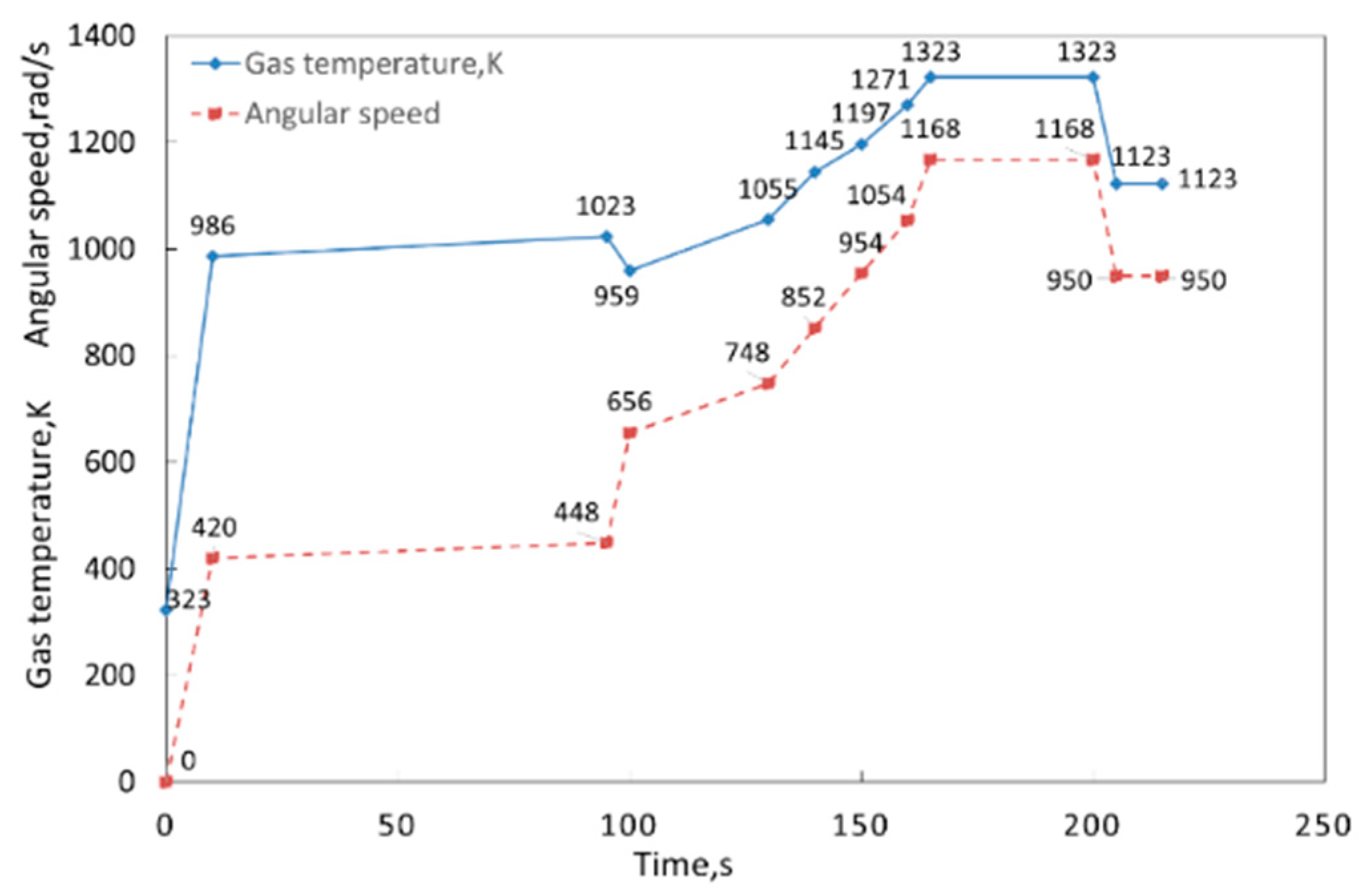
This paper selects the BTRRC of the first stage of the high-pressure turbine of an aeroengine as the object of study. In line with engineering experience, the flight profile of an aeroengine from start to cruise is considered as the analytical range in the time domain [0, 215 s] [9], in which 12 time points are selected as computing points. The flight profile is displayed in Figure 4.
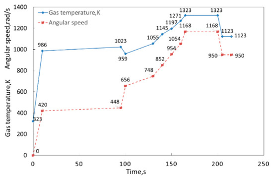
Figure 4.
Flight profile of aeroengine.
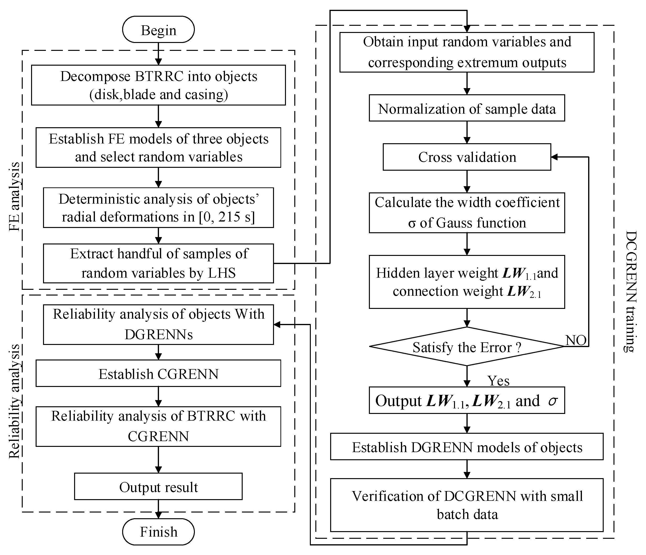
In line with the proposed DCGRENN method, the flowchart of the reliability analysis of BTRRC is structured in Figure 5 and is also summarized as follows:
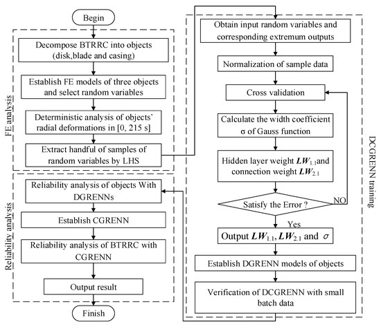
Figure 5.
The flowchart of BTRRC reliability analysis with DCGRENN method.
Step 1: Structure the FE models of the turbine disk, blades and casings through the decomposition of the BTRRC analysis problem into the radial creep problems of the three objects (disk, blade and casing);
Step 2: Implement the thermal-structural coupling deterministic analysis of the three objects in the time domain [0, 215 s] to acquire the change rule of BTRRC and determine the computing point with the minimum BTRRC by considering the input random variables (i.e., gas temperature, rotor speed, material parameters and convective heat transfer coefficient), the related boundary conditions, and multiple disciplines (i.e., heat load and centrifugal load);
Step 3: Extract the handful of samples for the random input variables by Latin hypercube sampling (LHS) technology [17], to perform FE analyses and obtain the creep deformations of the three objects (turbine disk, blade and casings) with respect to the samples, and regard the samples involving input parameters and the maximum values of the output responses as training samples;
Step 4: Normalize the training samples to obtain the optimal smooth factors, the weighted values in the hidden layer and the connection weights between the hidden layer and the output layer using the cross-validation method [31], and then structure the distributed generalized regression extremum neural network (DGRENN) models of three objects’ radial creep deformations;
Step 5: Check the precision of each object model. Return to Step 3 if the computational accuracy does not satisfy engineering requirements, or continue to Step 6;
Step 6: Conduct reliability analyses of the three objects’ radial creep deformations with the DGRENN models to obtain the distribution features of the maximum output responses;
Step 7: Establish the collaborative generalized regression extremum response surface (CGRENN) model (i.e., Equation (14)) of BTRRC by adopting coordinative method to coordinate the three DGRENN models;
Step 8: Implement the reliability analysis of BTRRC with the required CGRENN model by performing enough simulations and considering the creep deformations of the turbine disk, blades and casings as random input variables.
3.1. Finite Element Analysis
3.1.1. Finite Element Modeling
As shown in Figure 6, we decomposed the BTRRC structure into the structures of the turbine blade (Figure 6c), the disk (Figure 6d) and the casings (Figure 6b,e) [14], with respect to the DCGRENN method. Accordingly, the analysis of BTRRC analysis can be transformed into analyses of three objects’ deformations. Just like in Figure 6, the FE models of the three objects were built and meshed with hexahedral elements to generate 66,399 nodes and 16,413 cells for the disk, 26,266 nodes and 7333 cells for the blade and 66,183 nodes and 9180 cells for the casing. The turbine disk contains cooling holes and is cooled in operation. The symbols A1, A2, A3, B1, B2, and B3 indicate the different positions on the disk. The disk model was a simplified mortise structure and underwent symmetrical loads and boundary conditions. The mortise and cooling holes of the blade structure were ignored. B1, B2 and B3 denote the different areas of the blade. Due to the sensitivity of the casing bush ring on the deformation of casings and BTRRC, the bush ring was considered as the analyzed object to investigate casing creep deformation, in which the case model was divided into four segments: A, B, C and D.
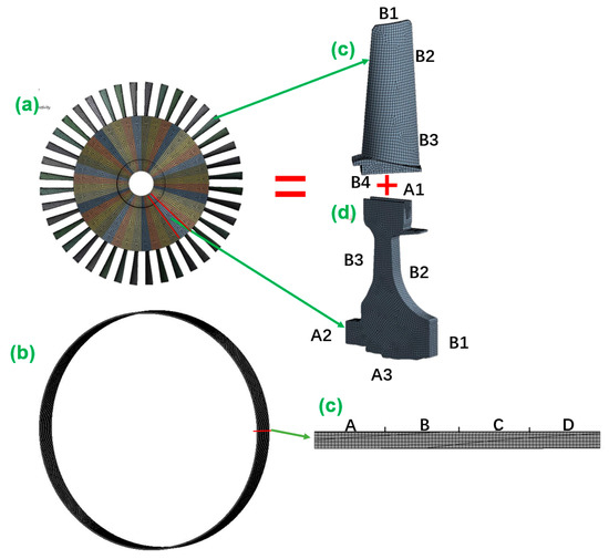
Figure 6.
Finite element models.
3.1.2. Selection of Random Variables
In this paper, many parameters, such as rotational speech ω, gas temperature T, heat conductivity coefficient λ, elasticity modulus E, convective heat transfer coefficient α, and material density ρ, are considered to be random input variables. These are assumed to be mutually independent and to follow normal distributions. The distribution characteristics of the variables are listed in Table 2. The temperatures and convective heat transfer coefficients on different positions on disk, blade and casing are computed according to the heat exchange between structures and gas temperature [14,18]. In the variables of the disk, the subscripts a1, a2, a3, b1 and b2 of T stand for the temperatures on the areas of A1, A2, A3, B1 and B2, respectively, and the subscripts d1, d2 and d3 of α indicate the convective heat transfer coefficients on B1, B2 and B3 on the disk model, respectively. For the variables of the blade, the subscripts b1, b2, b3 and b4 are the locations B1, B2, B3 and B4 on the blade model, respectively. In the variables of the casing, Ti and To are the temperatures inside and outside the casing rings respectively, and the subscripts c1, c2, c3, c4 and o of α indicate the convective heat transfer coefficients on segments A, B, C and D and the outside of casing ring.
Table 2.
The distributions of the random input variables.
3.1.3. Deterministic Analyses of Three Objects
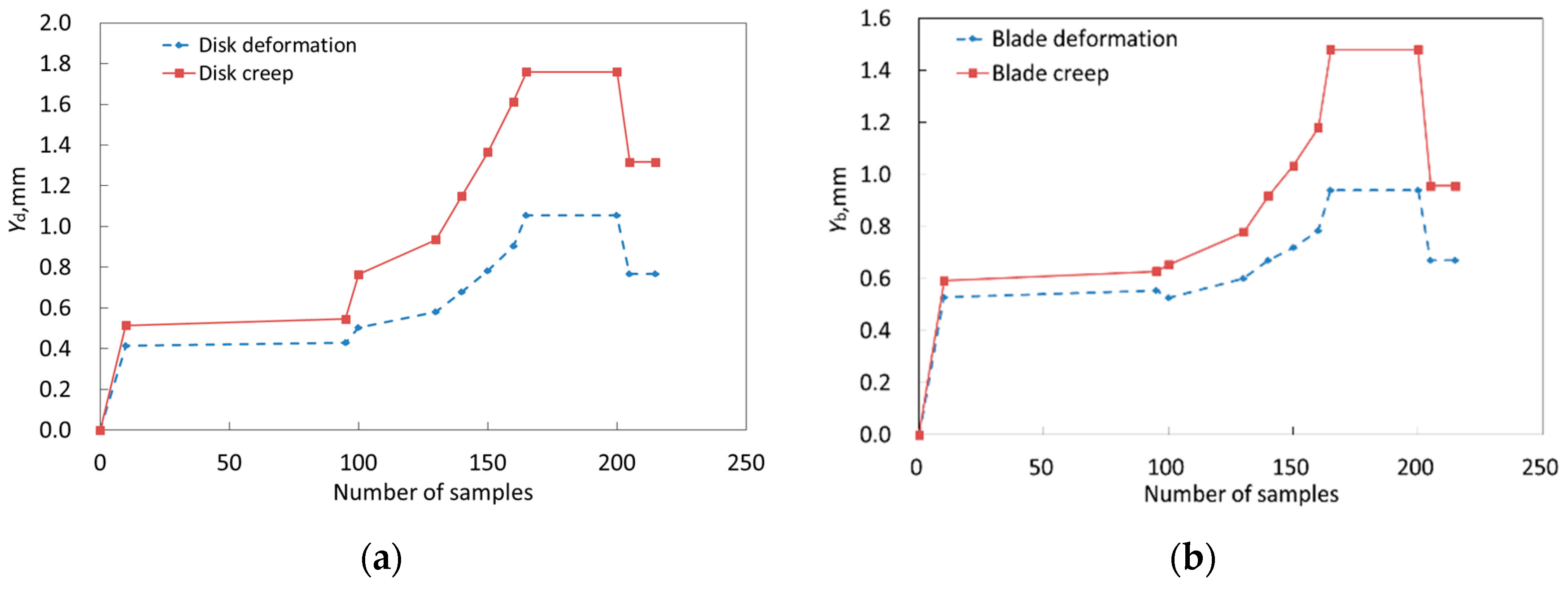
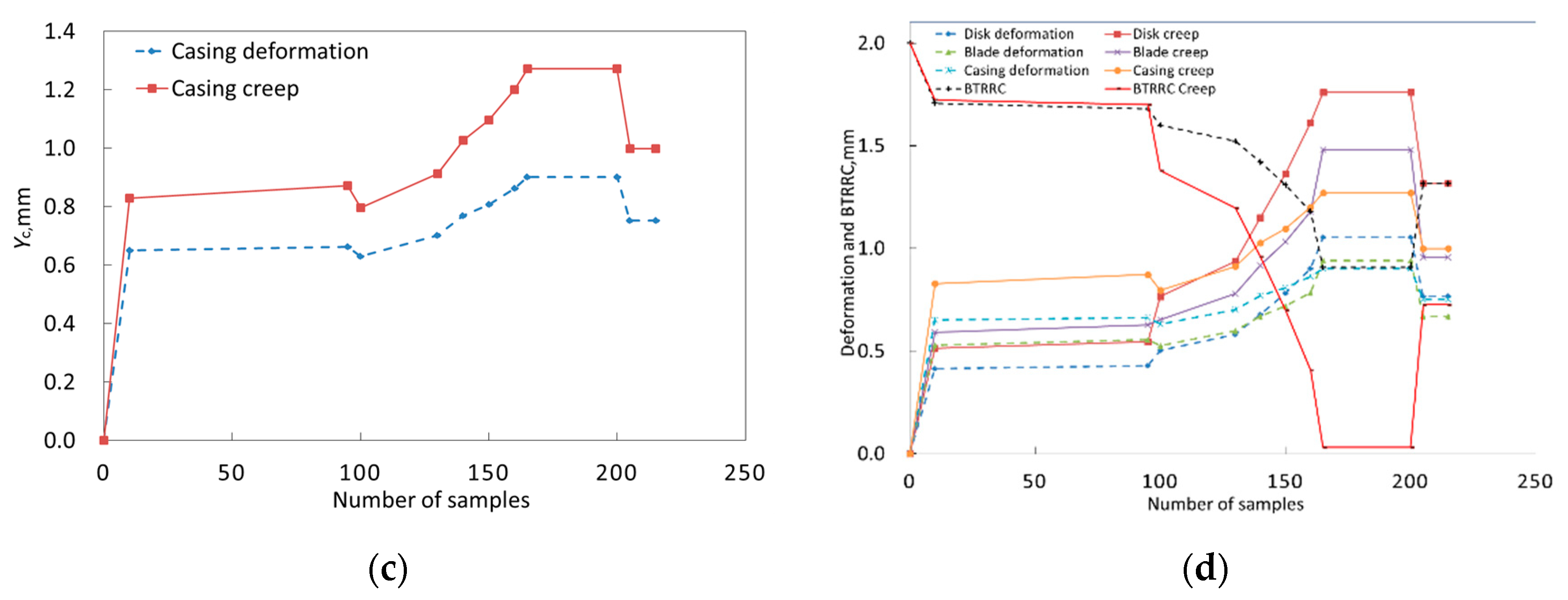
In the deterministic analysis of aeroengine BTRRC, the aerodynamic load was ignored because it is not significant in terms of its contribution to the stress for the turbine disk and casing, in comparison to the temperature load and the centrifugal load [32]. With reference to the flight profile of the aeroengine, the loads of heat and centrifugation and the nonlinearity of thermal expansivity, the means of variables in Table 2 were imported into the FE models in order to perform the thermo-structural coupling analysis of three objects under normal status, and to carry out the thermo-structural coupling analysis under creep. For the two analyses, the change curves of the disk, blade and casing deformations Yd(t), Yb(t) and Yc(t) with time are shown in Figure 7a–c. When the static blade-tip clearance δ = 2.0 mm, in line with Equations (12) and (13), the variation of BTRRC Y(t) with time are required in Figure 7d.
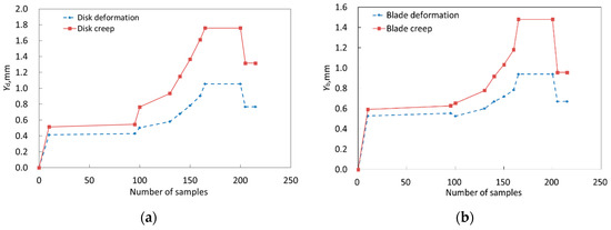
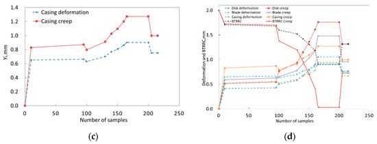
Figure 7.
The change of objects’ deformations and BTRRC: (a) disk, (b) blade, (c) casing, (d) BTRRC.
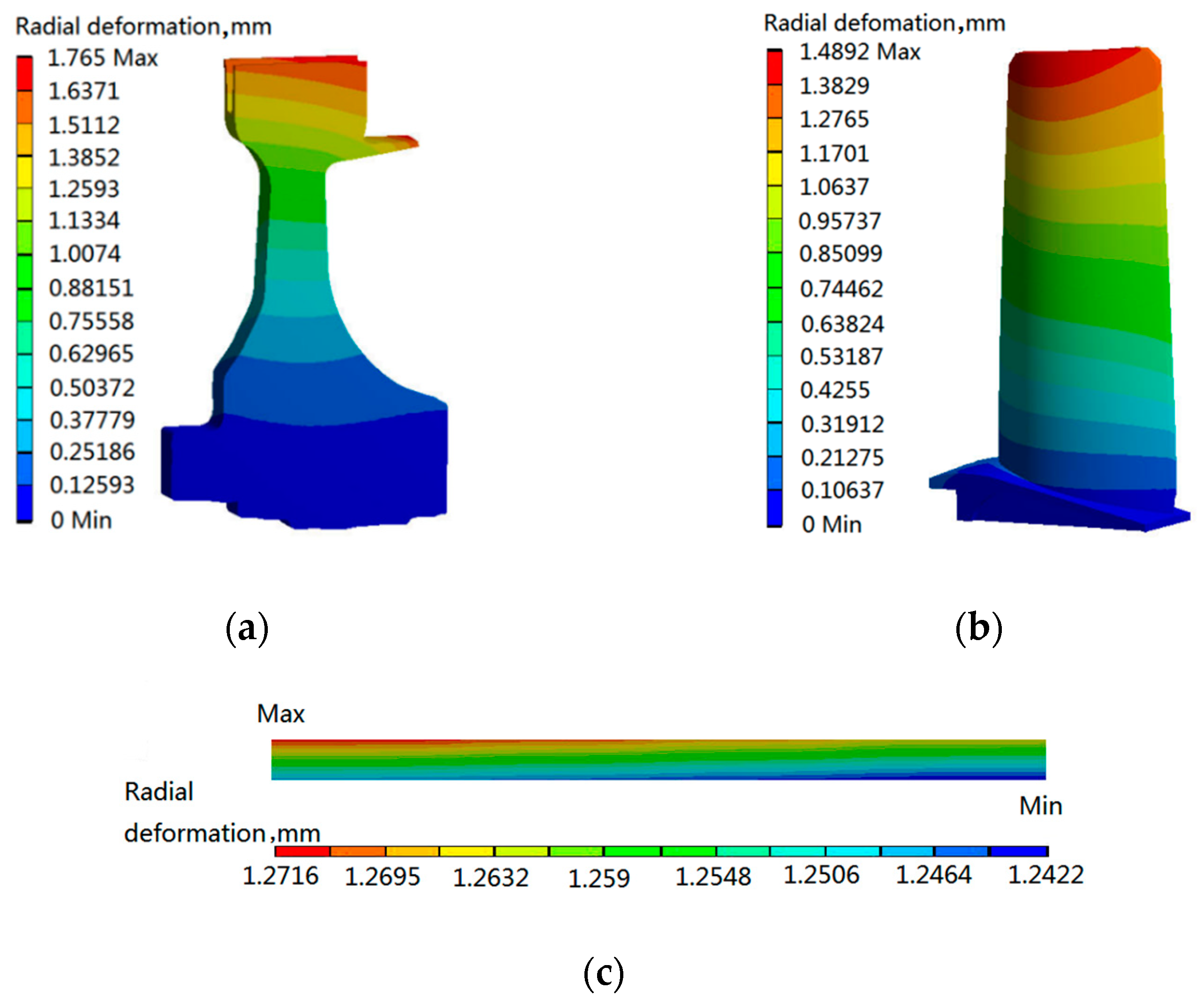
As illustrated in Figure 7, the creep seriously influences the BTRRC of aeroengine, and the BTRRC firstly decreases from start to cruise for the aeroengine. At t = 180 s, the BTRRC reaches its minimum and increases a bit when the aeroengine starts to cruise. Obviously, the dangerous point with respect to BTRRC occurs at t = 180 s, at which point gas temperature and rotational speech reach their maximum. The creep deformations of three objects at t = 180 s are shown in Figure 8.

Figure 8.
Distributions of creep deformations of disk, blade and casing at t = 180 s: (a) disk, (b) blade, (c) casing.
As revealed in Figure 8, at t = 180 s, the maximum creep deformations of the turbine disk, blade and casing were 1.765 mm, 1.4892 mm and 1.2716 mm. At that point in time, the maximum creep deformation of BTRRC is 1.9826 mm. Therefore, t = 180 s was selected as the computing point for BTRRC reliability analysis in this paper.
3.2. Modeling of the Distributed Collaborative Generalized Regression Extremum Neural Network
With respect to the distribution features of random variables in Table 2 and FE models, 150 samples for the maximum deformations of turbine disk, blade and casing were extracted by LHS technology as the pool of samples. From the pool of samples, 120 samples were selected as the training samples to establish the DGRENN models, and the remainder (30 samples) were the test samples for checking the developed DGRENN models.
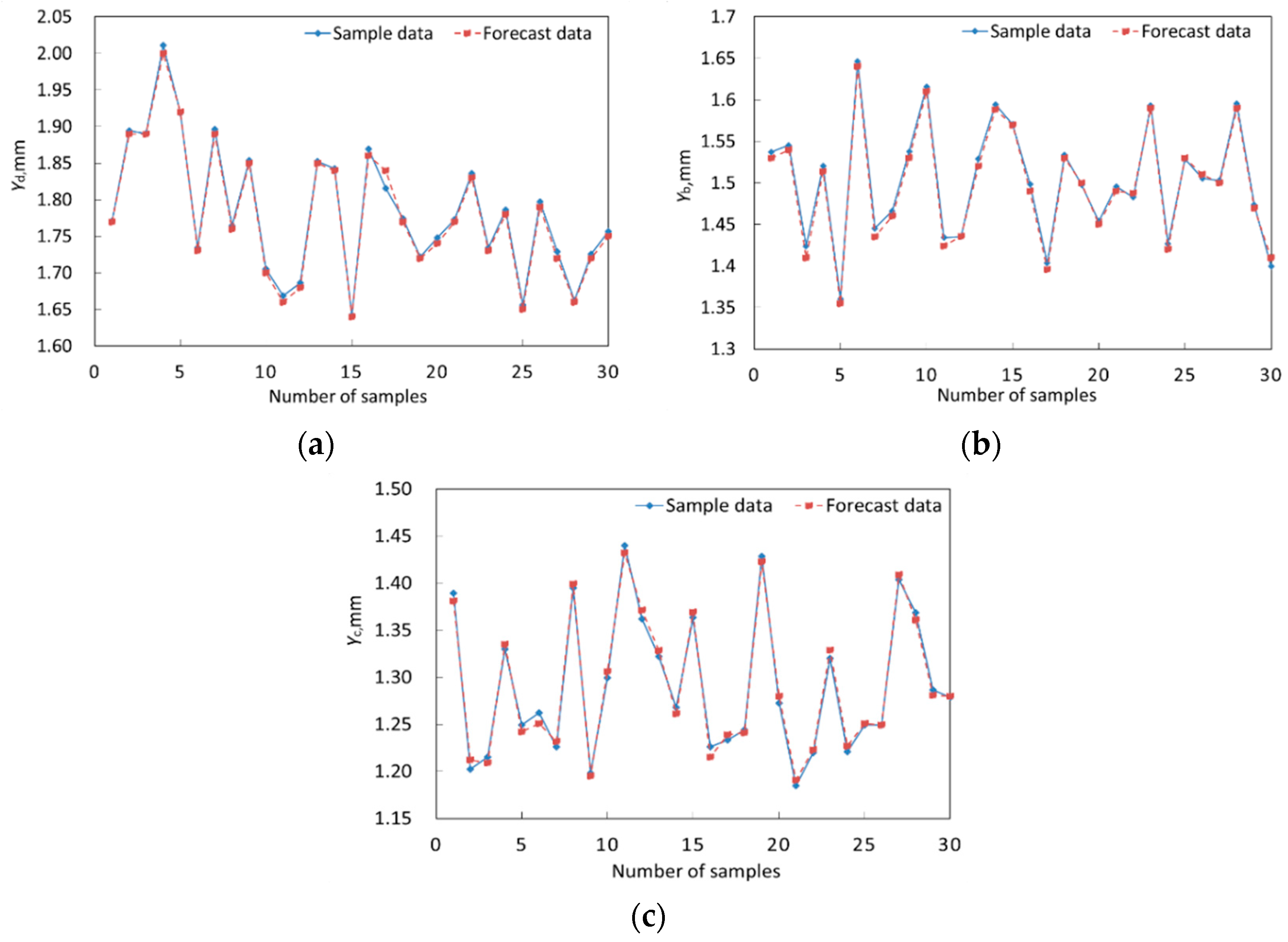
Along with the theory and concept of the DCGRENN method and BTRRC reliability analysis, in the GRENN model, the Gauss function is selected as the transfer function in the hidden layer, in which the weights matrix LW1,1 was computed using the Euclidean distance function [33,34,35]. Then the outputs of the hidden layer were regarded as the connected weights matrix LW2,1 of the hidden layer and the output layer. To avoid excessive modeling error, the data of the acquired samples were normalized. The normalized data were applied in order to train the DGRENN model by computing the parameters of DGRENN using the cross-validation method [31]. Finally, smooth factors of = 0.87, = 0.84 and = 0.76 were obtained, the weights matrix LW1,1 in the hidden layers of three objects (Yd, Yb and Yc), the weight matrix LW2,1 in the output layer, and the threshold matrix b, which are illustrated in Appendix A. By introducing the Appendix A, comprising three equations, into Equation (9), the DGRENN models were structured. The remaining 30 samples were employed to check the established DGRENN model. The prediction results are shown in Figure 9, and their root-mean-square errors (RMSEs) are listed in Table 3. It is revealed in Figure 9 and Table 3 that the predicted results are almost consistent with the original data due to small RMSE, indicating the effectiveness and accuracy of the presented DGRENN models.
Figure 9.
Comparison of prediction results with samples values (original data). (a) Disk, (b) blade, (c) casing.
Table 3.
DGRENN prediction evaluation with 30 testing samples.
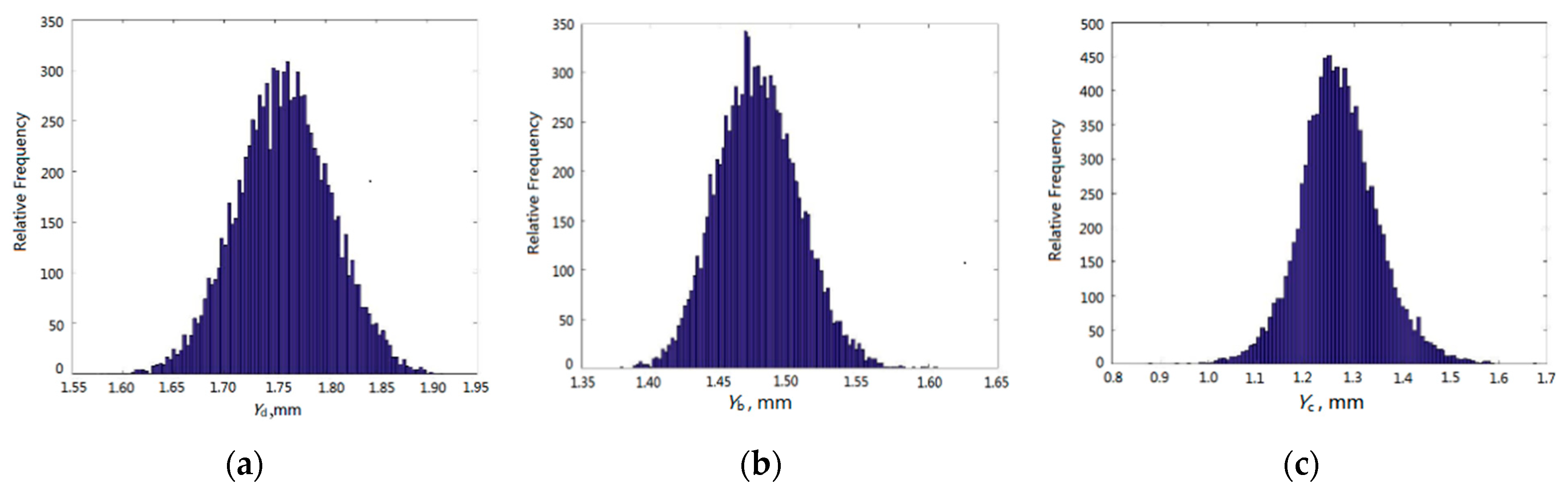
The DGRENN models, instead of the FE models, were simulated 104 times using the MC method in order to complete the dynamic probabilistic analysis of the three objects (disk, blade and casing) and then to acquire the creep deformations of objects. The histograms of creep deformations are shown in Figure 10 and the distribution features of Yd, Yb and Yc are displayed in Table 4.
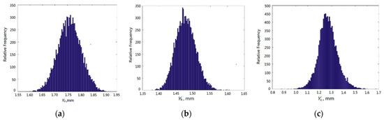
Figure 10.
The histograms of radial creep deformations of disk, blade and casing. (a) Disk creep deformation; (b) blade creep deformation; (c) casing creep deformation.
Table 4.
The distribution of the maximum creep deformations of disk, blade and casing.
3.3. Creep-Based Reliability Analysis
In line with the DCGRNN method, the creep deformations of three objects were considered as the inputs of BTRRC reliability analysis. Equations (12) and (14) are regarded as the CGRENN models of BTRRC probabilistic analysis with 104 simulations using the MC method. Based on this analysis, the history simulation graph, histogram and probabilistic cumulative graph of the maximum creep deformation of BTTRC at t = 180 s are shown in Figure 11.
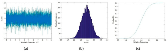
Figure 11.
The results of BTRRC reliability analysis using the DCGRENN method. (a) History simulation graph of τ, (b) histogram of τ, (c) cumulative probability graph of τ. Note: τ—the deformation of BTRRC.
As shown in Figure 11, the mean and standard deviation of BTRRC are 1.9829 mm and 0.07539 mm, respectively; the reliability degree of BTRRC is determined as 0.990 9 due to 91 failed simulations; and the analysis requires 1.216 s with a static blade-tip clearance δ = 2.2 mm. On the basis of engineering experience, these results are basically appropriate for BTRRC design and control.
3.4. Validation of Method
To validate the DCGRENN method, the reliability analyses of BTRRC were conducted using the MC method, the distribution collaborative response surface method (DCRSM) [18], and the DCGRENN method, in turn, under the same simulation conditions with random variables presented in Table 2 and using a computer with an Intel® Core™ i7-8400 processor and 16 GB RAM (Random Access Memory). The computing precision and the time required by the three methods were assessed under different simulations (102, 103, 104, 105 and 106) with static blade-tip clearance δ = 2.2 mm. The analytical results are listed in Table 5 and Table 6. The precision of BTRRC reliability degree was regarded to evaluate the precision of the methods, with the MC method acting as a reference in BTRRC reliability analysis. With respect to the 104 simulations, the computing precision in Table 6 is defined by
where is the reliability degree computed by MC method; is the reliability degree calculated by DCRSM or DCGRENN.
Table 5.
Computing time of different methods under different numbers of simulations.
Table 6.
Precision of different reliability methods under different numbers of simulations.
As seen in Table 5: (1) the computing time of the three method increases with the increase in the number of simulations, owing to the increase in the computing loads, wherein the increase for the DCGRENN method is slower than that of the other two methods. For instance, from 102 simulations to 106 simulations, the DCGRNN method only increased about two-fold, while the DCRSM increased more than 100-fold. Additionally, it is amazing that the MC method increased more than 100-fold from 102 simulations to 104 simulations; (2) DCRSM and DCGRENN required far less time that the MC method to carry out the same number of simulations, because surrogate model-based simulation is easier and faster than FE-based simulation. This is why the surrogate model was used to perform the reliability analysis of BTRRC in this study; (3) the MC method cannot conduct the probabilistic analysis of BTRRC when the number of simulations is larger than 104, due to the unaffordable computational burden. In this case, the results of 104 FE simulations were used as a reference for assessing the computational time and efficiency of the other methods in this study, because the credibility of reliability analysis is positively correlated the number of FE simulations in engineering reliability design; (4) the developed DCGRENN method showed greater computational efficiency than DCRSM, and the strength of the DCGRENN method was more obvious with the increase in the number of simulations, since the speed of GRNN in simulation is a result of its advantage of a small number of samples relative to quadratic polynomials.
As revealed in Table 6, the computing precision of DCGRENN method is higher than DCRSM, and improved by 1.23% over 104 simulations. It should be noted that the DCGRNN method is better able to ensure computing precision for small simulations. For example, the DCGRENN method is improved by 2.017% at 100 simulations. The reason for this is that the GRENN has good properties with respect to the handling of highly nonlinear and transient problems in structural dynamic probabilistic analysis, and the DC strategy is able to process MOMD analysis problems for complicated structures by reducing the nonlinearity.
In conclusion, the proposed DCGRENN method is able to improve the precision and efficiency of the reliability analysis of complex structures, in addition to the BTRRC, in aeroengines.
4. Conclusions
The aim of this paper was to develop a distributed collaborative generalized regression extremum neural network (DCGRENN) method by integrating the generalized regression extremum neural network with nonlinear fitting ability and a small numbers of samples with the distributed collaborative response surface method with multi-object multi-discipline coordinative capability. The developed approach is applied in order to improve the efficiency and precision of the simulations for the purpose of high-pressure blade-tip radial running clearance reliability analysis subject to creep behavior. The main conclusions are summarized as follows:
From the deterministic analysis of blade-tip clearance with creep, it is illustrated that the maximum creep deformations of the turbine disk, blade and casing were 1.765 mm, 1.4892 mm and 1.2716 mm at t = 180 s. At this moment, the maximum creep deformation of the blade-tip clearance was 1.9826 mm. This study selected t = 180 s as the computing point of the blade-tip clearance reliability analysis. The creep-based dynamic reliability analysis of the blade-tip clearance reveals that the creep deformation of blade-tip clearance obeys the normal distribution with the mean of 1.9829 mm and the standard deviation of 0.07539 mm, and the reliability degree of the blade-tip clearance was 0.9909 when the steady blade-tip clearance δ was 2.2 mm, which provides a significant reference for blade-tip clearance design in engineering.
With respect to computational efficiency, the method developed in this study was validated to have high computational efficiency in the dynamic probabilistic analysis of complex structures, thanks to the strengths of the generalized regression extremum neural network and the distributed collaborative strategy. With respect to computing precision, the proposed method was higher by 1.23% than the distributed collaborative response surface method under 104 simulations in blade-tip clearance reliability analysis, owing to the capabilities of the generalized regression extremum neural network in terms of addressing highly nonlinear analysis problems.
Author Contributions
Conceptualization, C.-Y.Z. and C.-W.F.; methodology, J.-S.W.; software, Z.W.; validation, Z.-S.Y., C.L., and C.-W.F.; formal analysis, C.L.; investigation, J.-S.W.; resources, C.-Y.Z.; data curation, C.-W.F.; writing—original draft preparation, C.-Y.Z. and J.-S.W.; writing—review and editing, C.-W.F.; visualization, Z.W.; supervision, C.-W.F. and C.-Y.Z.; project administration, C.-Y.Z.; funding acquisition, C.-Y.Z. and C.-W.F.
Funding
This research was funded by [the National Natural Science Foundation of China] grant number [51975124 and 51275138], [Start-up Research Funding of Fudan University] grant number [FDU38341] and [Excellent Doctorate Cultivating Foundation of Northwestern Polytechnical University] grant number [CX201932]. And the APC was funded by [51275138].
Conflicts of Interest
The authors declare no conflict of interest.
Acronyms
| Acronyms | Explanations |
| BTRRC | Blade-tip radial running clearance |
| MC | Monte Carlo |
| RSM | Response surface method |
| ERSM | Extremum response surface method |
| DC | Distributed collaborative |
| DCRSM | Distributed collaborative response surface method |
| DCERSM | Distributed collaborative extremum response surface method |
| GRNN | Generalized regression neural network |
| GRENN | Generalized regression extremum neural network |
| CGRENN | Collaborative generalized regression extreme neural network |
| DGRENN | Distributed generalized regression extreme neural network |
| DCGRENN | Distributed collaborative generalized regression extreme neural network |
| FE | Finite element |
| LHS | Latin hypercube sampling |
| RMSE | Root-mean-square error |
| SOSD | Single-object single-discipline |
| MOMD | Multi-object multi-discipline |
| RAM | Random access memory |
Nomenclature
| △εcreep | Creep strain |
| ε | Strain |
| t | Time |
| T | Test temperature |
| C1, C2, C3 | Coefficients of material creep |
| exp | Nature exponential function |
| X | Matrix of input samples |
| Q | Number of training samples |
| R | Dimension number of input parameters |
| S | Dimension number of output parameters |
| LW1.1 | Weighted matrix in hide layer |
| Q × R | Dimensions of matrix LW1.1 |
| ||dist|| | Weight (Euclidean distance) function in hide layer |
| △ | Transfer (Gauss) function |
| n1 | Network vector in hide layer |
| a1 | Output of neuro cell in hide layer |
| LW2.1 | Connection threshold value between hide layer and output layer |
| S × Q | Stands for the dimensions of matrix LW2.1 |
| nprod | Weight function of output layer |
 | Purelin transfer function of output layer |
| b | Threshold level vector |
| n2 | Network vector of output layer |
| a2 | Output of neuro cell in output layer |
| y | Output of neuro network |
| aj | Output vectorof Q nerve cells for jth group of input samples |
| The ith element in | |
| E | Mean value of blade-tip clearance |
| D | Variance of blade-tip clearance |
| μY(⋅) | Mean function |
| Disk mean value | |
| Blade mean value | |
| Casing mean value | |
| Disk variance value | |
| Blade variance value | |
| Casing variance value | |
| DY(⋅) | Variance function |
| R | Reliability |
| Φ(⋅) | Accumulative function |
| ω | Rotational speech |
| λ | Heat conductivity coefficient |
| E | Elasticity modulus |
| α | Convective heat transfer coefficient |
| ρ | Material density |
| σ | Smooth factors |
| δ | Allowable value of steady blade-tip clearance |
| γa | Reliability degree computed by MC method |
| γm | Reliability degree calculated by DCRSM or DCGRENN |
| Computing precision | |
| Yi | Output response of ith input sample in time domain [0, T] |
| Yi,max | The maximum of Yi(Xi,t) in time domain |
| i | Number of training samples |
| j | Number of random variables |
| X(pq) | Input sample vector of qth discipline in pth object |
| Y(pq) | Output sample vector of qth discipline in pth object |
| Weight matrix in hidden layer of output layer in the DGRENN model | |
| Weight matrix in output layer of output layer in the DGRENN model | |
| Output vector of output layer in the DGRENN model | |
| X(p) | Input random variables of pth object model |
| Y(q) | Response of pth object |
| Weight matrix in hidden layer of output layer in the DGRENN model | |
| Weight matrix in output layer of output layer in the DGRENN model | |
| Output vector of output layer | |
| Input random variables of the whole coordinative model | |
| Output response of MOMD overall CGRENN model | |
| Weight matrix in hidden layer of output layer | |
| Weight matrix in output layer of output layer | |
| Output vector of output layer in the CGRENN | |
| Radial deformations of turbine disk | |
| Radial deformations of turbine blade | |
| Radial deformations of turbine casings | |
| τ(t) | Deformation of BTRRC |
Appendix A
References
- Lattime, S.B.; Steinetz, B.M. Turbine engine clearance control systems: Current practices and future directions. J. Propuls. Power 2004, 20, 302–311. [Google Scholar] [CrossRef]
- Jia, B.H.; Zhang, X.D. Study on effect of rotor vibration on tip clearance variation and fast active control of tip clearance. Adv. Mater. Res. 2010, 139–141, 2469–2472. [Google Scholar] [CrossRef]
- Pilidis, P.; Maccallum, N.R.L. Models for predicting tip clearance changes in gas turbines. NASA 1983, N83–229258. [Google Scholar]
- Annette, E.N.; Christoph, W.M.; Stehan, S. Modeling and validation of the thermal effects on gas turbine transients. J. Eng. Gas Turbines Power 2005, 127, 564–572. [Google Scholar]
- Fei, C.W.; Bai, G.C. Nonlinear dynamic probabilistic analysis for turbine casing radial deformation based on extremum response surface method-based support vector machine. J. Comput. Nonlinear Dyn. 2013, 8, 041004. [Google Scholar] [CrossRef]
- Song, L.K.; Bai, G.C.; Fei, C.W.; Tang, W.Z. Multi-failure probabilistic design for turbine bladed disks using neural network regression with distributed collaborative strategy. Aerosp. Sci. Technol. 2019, 92, 464–477. [Google Scholar] [CrossRef]
- Fei, C.W.; Lu, C.; Liem, R.P. Decomposed-coordinated surrogate modelling strategy for compound function approximation and a turbine blisk reliability evaluation. Aerosp. Sci. Technol. 2019, 95, 105466. [Google Scholar] [CrossRef]
- Murat, E.K.; Hasan, B.B.; Aledar, B. Probabilistic nonlinear analysis of CFR dams by MCS using response surface method. Appl. Math. Model. 2011, 35, 2752–2770. [Google Scholar]
- Fei, C.W.; Tang, W.Z.; Bai, G.C. Novel method and model for dynamic reliability optimal design of turbine blade deformation. Aerosp. Sci. Technol. 2014, 39, 588–595. [Google Scholar] [CrossRef]
- Puatatsananon, W.; Saouma, V.E. Reliability analysis in fracture mechanics using the first-order reliability method and Monte Carlo simulation. Fatigue Fract. Eng. Mater. Struct. 2010, 29, 959–975. [Google Scholar] [CrossRef]
- Pan, Q.; Dias, D. An efficient reliability method combining adaptive support vector machine and Monte Carlo simulation. Struct. Saf. 2017, 67, 85–95. [Google Scholar] [CrossRef]
- Fei, C.W.; Bai, G.C.; Tian, C. Extremum response surface method for casing radial deformation probabilistic analysis. J. Aerosp. Inf. Syst. 2013, 10, 47–52. [Google Scholar]
- Wei, Z.; Feng, F.; Wei, W. Non-linear partial least squares response surface method for structural reliability analysis. Reliab. Eng. Syst. Saf. 2017, 161, 69–77. [Google Scholar]
- Fei, C.W.; Choy, Y.S.; Hu, D.Y.; Bai, G.C.; Tang, W.Z. Dynamic probabilistic design approach of high-pressure turbine blade-tip radial running clearance. Nonlinear Dyn. 2016, 86, 205–223. [Google Scholar] [CrossRef]
- Song, L.K.; Bai, G.C.; Fei, C.W.; Wen, J. Probabilistic LCF life assessment of turbine discs using DC-based wavelet neural network regression. Int. J. Fatigue 2019, 119, 204–219. [Google Scholar] [CrossRef]
- Zhang, C.Y.; Bai, G.C. Extremum response surface method of reliability analysis on two-link flexible robot manipulator. J. Cent. South Univ. 2012, 19, 101–107. [Google Scholar] [CrossRef]
- Lu, C.; Feng, Y.W.; Liem, R.P.; Fei, C.W. Improved kriging with extremum response surface method for structural dynamic reliability and sensitivity analyses. Aerosp. Sci. Technol. 2018, 76, 164–175. [Google Scholar] [CrossRef]
- Bai, G.C.; Fei, C.W. Distributed collaborative response surface method for mechanical dynamic assembly reliability design. Chin. J. Mech. Eng. 2013, 26, 1160–1168. [Google Scholar] [CrossRef]
- Zhang, C.Y.; Wang, Z.; Fei, C.W.; Yuan, Z.S.; Wei, J.S.; Tang, W.Z. Fuzzy Multi-SVR Learning Model for Reliability-Based Design Optimization of Turbine Blades. Materials 2019, 12, 2341. [Google Scholar] [CrossRef]
- Fei, C.W.; Choy, Y.S.; Hu, D.Y.; Bai, G.C.; Tang, W.Z. Transient probabilistic analysis for turbine blade-tip radial clearance with multiple components and multi-physics fields based on DCERSM. Aerosp. Sci. Technol. 2016, 50, 62–70. [Google Scholar] [CrossRef]
- Nosefilho, K.; Plasencia, L.A.D.; Minussi, C.R. Short-term multinodal load forecasting using a modified general regression neural network. IEEE Trans. Power Deliv. 2011, 26, 2862–2869. [Google Scholar] [CrossRef]
- Adel, M.E.; Salah, G.F. EOS simulation and GRNN modeling of the constant volume depletion behavior of gas condensate reservoirs. Energy Fuels 1998, 12, 353–364. [Google Scholar]
- Zhao, C.; Liu, K.; Li, D.S. Freight volume forecast based on GRNN. J. China Railw. Soc. 2004, 10, 112–113. [Google Scholar]
- Machado, R.N.D.M.; Bezerra, U.H.; Pelaes, E.G.; Oliveira, R.C.L.D.; Tostes, M.E.D.L. Use of wavelet transform and generalized regression neural network (GRNN) to the characterization of short-duration voltage variation in electric power system. IEEE Lat. Am. Trans. 2009, 7, 217–222. [Google Scholar] [CrossRef]
- Li, H.Z.; Guo, S.; Li, C.J.; Sun, J.Q. A hybrid annual power load forecasting model based on generalized regression neural network with fruit fly optimization algorithm. Knowl. Based Syst. 2013, 37, 378–387. [Google Scholar] [CrossRef]
- Zhang, C.Y.; Wei, J.S.; Jing, H.Z.; Fei, C.W.; Tang, W.Z. Reliability-based low fatigue life analysis of turbine blisk with generalized regression extreme neural network method. Materials 2019, 12, 1545. [Google Scholar] [CrossRef]
- Sun, G.; Hoff, S.J.; Zelle, B.C.; Smith, M.A. Development and comparison of backpropagation and generalized regression neural network models to predict diurnal and seasonal gas and PM 10 concentrations and emissions from swine buildings. Trans. Asabe 2008, 51, 685–694. [Google Scholar] [CrossRef]
- Ibanez, A.R.; Srinivasan, V.S.; Saxena, A. Creep deformation and rupture behaviour of directionally solidified GTD 111 superalloy. Fatigue Fract. Eng. Mater. Struct. 2010, 29, 1010–1020. [Google Scholar] [CrossRef]
- Zeng, S.Q.; Zhang, Z.J. The Forced Creep Analysis of Nonmetallic Material. Appl. Mech. Mater. 2012, 1841–1885, 692–695. [Google Scholar] [CrossRef]
- Liu, Y.; Ning, Y.; Nan, Y. Characterization of hot deformation behavior and processing map of FGH4096-GH4133B dual alloys. J. Alloy. Compd. 2015, 633, 505–515. [Google Scholar] [CrossRef]
- Jeon, J.; Panagiotelis, A.; Petropoulos, F. Probabilistic forecast reconciliation with applications to wind power and electric load. Eur. J. Oper. Res. 2019, 279, 364–379. [Google Scholar] [CrossRef]
- Shu, M.A.; Wang, K.M.; Hui, M.; Shuai, Z. Research on turbine blade vibration characteristic under steady state temperature field. J. Shenyang Aerosp. Univ. 2011, 28, 18–21. [Google Scholar]
- Manduhu, M.; Jones, M.W. A work efficient parallel Algorithm for exact Euclidean distance transform. IEEE Trans. Image Process. 2019, 28, 5322–5335. [Google Scholar] [CrossRef] [PubMed]
- Song, L.K.; Bai, G.C.; Fei, C.W. Dynamic surrogate modeling approach for probabilistic creep-fatigue life evaluation of turbine disks. Aerosp. Sci. Technol. 2019, 95, 105439. [Google Scholar] [CrossRef]
- Zhang, C.Y.; Yuan, Z.S.; Wang, Z.; Fei, C.W.; Lu, C. Probabilistic fatigue/creep optimization of turbine bladed disk with fuzzy multi-extremum response surface method. Materials 2019, 12, 3367. [Google Scholar] [CrossRef]


© 2019 by the authors. Licensee MDPI, Basel, Switzerland. This article is an open access article distributed under the terms and conditions of the Creative Commons Attribution (CC BY) license (http://creativecommons.org/licenses/by/4.0/).