Abstract
In this paper, a semi-analytical method is adopted to analyze the free vibration characteristics of composite laminated shallow shells under general boundary conditions. Combining two kinds of shell theory, that is, first-order shear deformation shell theory (FSDT) and classical shell theory (CST), to describe the dynamic relationship between the displacement resultants and force vectors, the theoretical formulations are established. According to the presented work, the displacement and transverse rotational variables are transformed into wave function forms to satisfy the theoretical formulation. Related to diverse boundary conditions, the total matrix of the composite shallow shell can be established. Searching the determinant of the total matrix using the dichotomy method, the natural frequency of composite laminated shallow shells is obtained. Through several classical numerical examples, it is proven that the results calculated by the presented method are more accurate and reliable. Furthermore, to discuss the effect of geometric parameters and material constants on the natural frequencies of composite laminated shallow shells, some numerical examples are calculated to analyze. Also, the influence of boundary elastic restrained stiffness is discussed.
1. Introduction
The shallow shell is an open shell with a small curvature and radius of curvature compared with various shell parameters (i.e., length and width). With the development research into composite materials, composite laminated shallow shells are widely applied in some modern engineering practice with a high level of intensity and rigidity, for instance, petroleum equipment, aerospace equipment, and marine equipment. It is worth noting that the composite laminated shallow shells are typically operated under complicated environmental conditions and subjected to complex boundary conditions. So, it is particular importance to fully investigate the free vibration characteristics of composite laminated shallow shells with non-classical boundary conditions.
Through many years of hard work by research scholars, some shell theories have been summarized, such as classical shell theory (CST) [1,2,3], first-order shear deformation shell theory (FSDT) [4,5], and high-order shell theory (HST) [6,7,8,9,10]. CST is the basic shell theory and is known as the simplest equivalent single layer, which is based on the Kirchhoff–Love hypothesis. To analyze the complex shell structure, some shell theories were developed along with some assumptions, such as Reissner–Naghdi’s shell theory and Donner–Mushtari’s theory. A more detailed description of these theories can be found in the research by Reddy [11], Leissa [12], and Qatu [13]. The main application area is thin shell structures. To analyze the thick shell, CST ignores the effect of transverse shear deflection, causing the calculation of natural frequencies to be inaccurate. To improve the influential impact of transverse shear deformation, FSDT is conducted. HST can attenuate the dependence of FSDT on shear correction factors; however, there is a large amount of calculation in the study of the high-order stress resultant force. Simultaneously, many remarkable researchers have investigated the composite laminated shallow shell in recent years and published some excellent papers. Ye et al. [14] investigated the free vibration characteristics of the composite laminated shallow shell under general elastic boundary conditions. The closed form auxiliary functions are used to transform the displacement variables into standard Fourier cosine series. Kurpa et al. [15] extended the R-function method to investigate the composite laminated shallow shells on an arbitrary planform by FSDT. Fazzolari and Carrera E [16] conducted the Ritz formulation and Carrera unified formulation to investigate the composite laminated doubly-curved anisotropic shell, and the free vibration response is discussed. Awrejcewicz et al. [17] proposed R-functions theory and the spline-approximation to study the bending performance of the composite shallow shell with a static loading boundary condition. Tran et al. [18] presented a static feature of the cross-ply composite hyperbolic shell panels on Winkler–Pasternak elastic foundation, and the smeared stiffeners technique was adopted. Biswal et al. [19] discussed the free vibration characteristic of composite shells consisting of woven fiber glass/epoxy with hygrothermal environments. The FSDT and quadratic eight-noded isoparametric element are adopted to study the free vibration characteristics under elevated temperatures and moisture concentrations conditions. Garcia et al. [20] investigated the effect of polycaprolactone nanofibers on the dynamic behavior of glass fiber reinforced polymer composites. Garcia et al. [21] investigated the influence of the inclusion of nylon nanofibers on the global dynamic behaviour of glass fibre reinforced polymer (GFRP)composite laminates. Shao et al. [22] conducted the enhanced reverberation-ray matrix (ERRM) method to investigate the transient response of the composite shallow shell. In these studies, the kinetic analysis of composite laminated shallow shell is proposed to free vibration, and many analytical and computational methods were developed.
These include the Ritz method [23,24,25,26,27], dynamic stiffness method [28], closed-form solution [29,30,31], boundary domain element method [32], Meshfree approach [33], Galerkin method [34,35], and finite element method [36,37,38].
In recent years, the wave-based method (WBM) has been adopted to investigate the dynamic behavior of engineering structures in some applications. WBM was first proposed in the work of [39] to analyze the coupled vibro-acoustic systems and the steady-state dynamics characteristics of the system concerned. Deckers et al. [40] presented a literature review of WBM research for 15 years. With the research on structural vibration in recent years, WBM has been adopted in the dynamic analysis for some engineering structures, such as the dynamic characteristics of cylindrical shell structures, which many researchers have studied using WBM. Chen et al. [41] analyzed the free and force vibration characteristics of a cylindrical shell in discontinuity thickness form. Xie et al. [42] conducted WBM to study the free vibration and acoustic dynamic characteristics of underwater cylindrical shells with bulkheads. Wei et al. [43] investigated the non-uniform stiffener distribution of a cylindrical shell. At the same time, as many reinforcements and coupling structures are more common in engineering applications, the corresponding research is increasing, such as the cylindrical shell coupled elastically with annular plate and the ring stiffened cylindrical shell with frame ribs [44,45]. Also, the free vibration characteristics of the composite laminated cylindrical shell have been investigated [46]. Therefore, it is meaningful to develop an effective method for the general processing ability of composite laminated shallow shells with general boundary conditions. According to the author’s literature review of related topics, there has not been any published work with regard to the application of the presented method to analyze the free vibration characteristics of the composite laminated shallow shell with general boundary conditions.
For the first time, the wave-based method is adopted to study the free vibration characteristics for a composite laminated shallow shell with general boundary conditions. According to the relationship between the displacement vector and force resultants, the governing equation of composite shells is established by FSDT and CST. By converting the displacement variable into a wave function form and the boundary matrices, the total matrix is established. Solving the root of the total matrix determinant using the dichotomy method, the natural frequencies of composite laminated shallow shells are calculated. To verify the correctness of the solutions by the presented method, the comparisons of the current solutions with the results in represented literatures are shown. Furthermore, the influence of material parameters and geometric constants, such as length to radius ratios, length to thickness ratios, modulus ratios, and elastic restrained constants, are discussed in some numerical examples. The main purpose of this paper is to provide a relatively new method for analyzing the free vibration characteristics of composite laminated shallow shells, which provides a new direction for composite laminated structure analysis. When studying the vibration analysis of the composite laminated shallow shell with general boundary conditions, it is easier to obtain the total matrix, and the boundary conditions are easy to replace. The advantages of the presented method lie in its simplicity, low computational cost, and high precision.
2. Theoretical Formulations
2.1. The Description of Model
In Figure 1a, the schematic diagrams of the composite laminated shallow shells under elastic restraint are shown. Lx, Ly, and h express the length, width, and thickness, respectively, of the composite laminated shallow shells. Rx and Ry indicated the principle curvature radii. In the middle surface of the model, a global coordinate (o-xyz) is established in the length, width, and thickness directions. For the kth layer of the composite shell, the distances of top and bottom surface to the middle surface are denoted as Zk+1 and Zk. For the elastic boundary conditions, there is one set of linear springs (Ku, Kv, and Kw) and one pair of rotational springs (Kϕx and Kϕy), which set on two edges, x = 0 and Lx. Through the changing of two pairs of elastic restrained springs, an arbitrary elastic boundary condition can be achieved. In Figure 1b, with the changing of the principle curvature radii, the composite laminated shallow shells have various types, such as plate (i.e., Rx = Ry = ∞), cylindrical shell (i.e., Rx = R, Ry = ∞), spherical shell (i.e., Rx = Ry = R), and hyperbolic paraboloidal shell (i.e., Rx = −Ry = R).
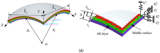
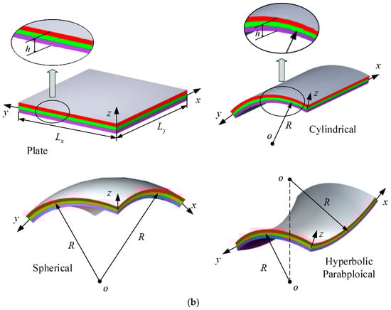
Figure 1.
(a): Geometric model of the composite laminated shallow shell with elastic restraint; (b): geometric model of the composite laminated shallow shell with various curvature types.
2.2. First-Order Shear Deformation Shell Theory (FSDT)
2.2.1. Kinematic Relations and Stress Resultants
This section is divided into subheadings. It should provide a concise and precise description of the experimental results and their interpretation, as well as the experimental conclusions that can be drawn.
According to the relationship between the displacement variables and rotation transverses of the composite shallow shells by FSDT, the displacement variables are shown as follows [13]:
where u0, v0, and w0 are the displacements of the arbitrary point along the x, y, and z directions, respectively, in the middle surface. ϕx and ϕy are the y and x axes transverse rotations, respectively, and t is a time variable. The linear strain relationship between the change strain and curvature in the middle surface under the assumption of small deformation is given as follows:
where {, } are the normal strains of the middle surface, {, , } are the shear stains, and {, , } are the curvature and twisting changes of the middle surface. The detailed expressed formulations of the strains and changes are defined as follows:
The corresponding stresses expressed by the Hooke’s law are as follows:
where (i, j = 1,2,4,5,6) are the transform coefficients and depend on material parameters; and the constants Qij (i,j = 1,2,4,5,6), which are associated with the strains and stresses, can be expressed as follows:
where E1, E2 are the Yong’s moduli and μ12 and μ21 are the Poisson’s ratios. By integrating the stresses and moments over the cross section and thickness, the relationship between the strains and curvature in the middle surface is given as follows:
where {Nxx, Nxy, Nyy} is the in-plane force resultant, {Mxx, Myy, Mxy} is the bending and twisting moment resultant, and {Qx, Qy} is the transverse shear force resultant. Kc is the shear correction factor and the value is set as 5/6. Furthermore, the stretching stiffness coefficients, coupling stiffness coefficients, and bending stiffness coefficients are given as follows:
where N is the number of the layers. Zk+1 and Zk are the distance from the top surface and bottom surface, respectively, to the middle surface of the kth layer. For analysis of the general cross-ply composite laminates shallow shell, the transform coefficients , and are zero. So, the corresponding stiffness coefficients will be vanished
2.2.2. Wave Function Solutions
The theoretical equations of the composite shell based on FSDT are given as follows [13]:
where Ii (i = 0, 1, 2) are the inertia mass moments. Submitting Equations (3) and (6) into Equation (8), the force vector and moment resultants can be transformed as displacement variables. Furthermore, the theoretical equations are follows:
where Tij (i,j = 1, 2, 3, 4, 5) are the operators of the matrix T in Equation (9), and are shown as follows:
For certain cross-ply composite laminated shallow shells under shear diaphragm boundary conditions, which are set at the opposite supports y = 0 and Ly (u0 = w0 = ϕx = Nyy = Myy = 0), the generalized displacement variables are transformed in the wave function form as follows:
where Ky = nπ/Ly is the y direction modal wave number and kn is the wave number in the x direction. U0, V0, W0, Φx, and Φy are the corresponding displacement amplitude variables of the nth mode for the composite laminated shallow shells.
Submitting the wave function solutions of the displacement variables into Equation (9), the governing equation can be obtained as follows:
where Lij (i,j = 1, 2, 3, 4, 5) are the governing equation coefficients of Equation (12), given as follows:
The solutions of Equation (12) can be solved and the determinant of the matrix T equal to zero. The characteristics equation of axial wavenumber kn is shown as follows:
There is a fifth-order equation of and λ10, λ8, λ6, λ4, λ2, and λ0 are the coefficients, which depend on the coefficient matrix T. There are ten characteristic axial wavenumbers to be obtained as ±kn,1, ±kn,2, ±kn,3, ±kn,4, and ±kn,5. Through the characteristic axial wavenumbers ±kn,i (i = 1, 2, 3, 4, 5), the corresponding basic solution vector is defined as follows:
The coefficients in Equation (15) are defined as follows:
where Ω and Ωi (i = 1, 2, 4, 5) are given as follows:
On the basis of the generalized displacement variables being transformed in the wave function form in Equation (11), related to the basic solution vector in Equation (15), the generalized displacement variables are shown in the matrix form:
where δn = {u, v, w, ϕx, ϕy}T is the generalized displacement resultant; Yn(y) is the modal matrix in the y direction; Dn is the coefficient matrix of the displacement resultant; Pn(x) is the axial wavenumber matrix; and Wn is the wave contribution factor resultant. The detailed expression of them is given as follows:
where ns is the number of characteristics roots of axial wavenumber in Equation (14). Also, the generalized force resultant fn = {Nxx, Nxy, Qx, Mxx, Mxy}T can refer to the constitutive relationship in Equations (3) and (6), as follows:
where the coefficient matrix Fn of force resultant fn is given as follows:
2.3. Classical Shell Theory (CST)
2.3.1. Kinematic Relations and Stress Resultants
For the integrity of the paper, the governing equations and wave function solutions in the CST are given. On the basis of the theoretical technique of FSDT, the governing equation can refer to CST by setting the slope of the rotation components ϕx and ϕy close to the transverse normal, as follows [12,13]:
2.3.2. Wave Function Solutions
In CST, the shear deformation in the kinematics equation is negligible, and the in-plane displacement can be expressed as a linear change in the thickness direction of the shallow shell. So, the governing equation can be given as follows [13]:
where
Submitting the generalized displacement variables in CST, the governing equation can be expressed as follows:
where (i,j = 1, 2, 3) are the operators, which are shown as follows:
For the generalized displacement functions of cross-ply composite laminated shallow shell with shear diaphragm boundary conditions, which are set as opposite support edges y = 0 and Ly (u0 = w0 = Nyy = Myy = 0), the displacement variables can be shown in the wave functions form:
Submitting Equation (30) into Equation (28), the governing equation can transform into the matrix form as follows:
where (i,j = 1, 2, 3) are the governing equation coefficients, as follows:
Next, the corresponding basic solution vector is set as {ξn,i, ηn,i, 1}T, and the detailed expression of the vector is given as follows:
where
On the basis of the basic solution vector, the displacement resultant δn = {u, v, w, ϕx}T and force resultant fn = {Nxx,Nxy + Mxy/Ry,Qx + ∂Mxy/∂y,Mxx}T are expressed as follows:
where
in which the coefficients Fn,ji(j = 1–4,i = 1–ns) are given as follows:
2.4. Implementation of the WBM
Through the introduction of the generalized displacement and force resultant, the final governing equations are assembled by the generalized displacement coefficient matrix, generalized force coefficient matrix, and boundary matrix. The final governing equation of the whole structure is defined as follows:
where F is the external force vector and is related to the external situation; when analyzing the free vibration dynamic, the external force F should vanish. W = {W1, W2}T is the wave contribution factor resultant of the composite shell, and Wi = {Wi,1, Wi,2,…, Wi,ns}T(i = 1, 2) is the wave contribution factor vector and is associated with the boundary conditions at x = 0 and x = L. K is the total matrix and the detailed expression of the matrix is shown as follows:
For the classical boundary conditions, the boundary matrix can be shown as follows:
where Tδ and Tf are the transform matrix of boundary matrix, as follows:
Free edge (F):
Clamped edge (C):
Shear-diaphragm edge (SD):
For the elastic boundary conditions, the boundary condition matrix B1(x) and B2(x) are given as follows:
where Kδ is the stiffness transform matrix and the detailed expression about it is as follows:
When the composite shell is under elastic restraint in the axial direction, the stiffness transform matrix Kδ is given as follows:
where {Ku, Kv, Kw } are linear springs and {Kϕx, Kϕy } are rotational springs, which are set in various directions. When the other displacements are under elastic restraint, the stiffness transform matrix Kδ is given as follows:
Through the introduction of the boundary conditions B1(x) and B2(x), which include the classical and elastic boundary conditions, the total matrix K is established. When analyzing the free vibration characteristics, the external force vector F vanishes. When calculating the natural frequencies, a series of the total matrix determinant is obtained. Using the dichotomy method to search the zeros position of the total matrix determinant, the natural frequency will be obtained with each circumferential mode number n. Through the numerical dichotomy method when the sign changed, the location of the total matrix K determinant is calculated and the natural frequencies can be obtained. Furthermore, to analyze the free vibration characteristics of the composite laminated shallow shell with arbitrary boundary conditions, the shell structure is considered to be calculated as a whole model and the displacement variable solutions are set as infinite wave function forms; the convergence study of the truncated number does not need to be considered. Thus, the computational cost of the present approach is low.
3. Numerical Examples and Discussion
Through the description of the theory formulation with FSDT and CST, the free vibration characteristics of composite laminated shallow shell with arbitrary classical boundary conditions, elastic boundary conditions, and their combinations are analyzed by WBM. In this part, some numerical examples are listed to verify the correctness of the results by WBM through the comparison with the presented results. Also, some numerical examples are presented to study the influence of the material parameters and geometric constants on the natural frequencies of composite laminated shallow shells with general boundary conditions.
3.1. Composite Laminated Shallow Shell with Classical Boundary Conditions
In this section, the free vibration characteristics of composite laminated shallow shells with arbitrary classical boundary conditions are concerned. Through the introduction of the boundary transform matrix Tδ and Tf, arbitrary classical boundary conditions can transform into boundary matrices B1(x) and B2(x) to investigate the free vibration characteristics of composite shallow shell with classical boundary conditions. In order to verify the correctness of the calculation by the presented method, some numerical examples are selected for verification. At the same time, the selected material parameters and geometric parameters are consistent with the examples in the comparative literatures.
First, the composite laminated shallow shell with full shear diagram boundary condition is concerned. In Table 1 and Table 2, the fundamental frequency parameters for three type cross-ply composite laminated shallow shells (i.e., cylindrical shell, spherical shell, and hyperbolic paraboloidal shell) with various radius to length ratios Ry/Ly (i.e., Ry/Ly = 2, 5, 10) under Shear-diaphragm boundary condition (SD-SD) by FSDST and CST are presented. Three kinds of cross-ply type layered composite shells (i.e., [0°/90°/90°/0°], [0°/90°], and [90°/0°]) are concerned. The material parameters and geometric constants are given as follows: Lx = 1 m, Ly/Lx = 1, h/Ly = 0.01 and 0.1, E2 = 7 GPa, E1/E2 = 15, G12 = G13 = 0.5E2, G23 = 0.5E2, μ12 = 0.25, ρ = 1650 kg/m3. The presented results compare with the results by Qatu [13] and Shao et al. [22]. From Table 1 and Table 2, the presented results by WBM match well with the results in the presented literatures. The maximum divergence is −4.61% with the situation Ry/Ly = −1 for the [90°/0°] cross-ply composite laminated paraboloidal shell. It is obvious that the errors in Table 2 by CST are lower than the errors in Table 1 by FSDT. Also, from Table 1, it can be found that, with the radius to length ratios Ry/Ly from 2 to 10 for the composite shallow shell with the lamination schemes 0°/90°/90°/0° and 0°/90°, the errors between the solutions by the presented method those of the the results in the literature by Quta are generally growing. This is caused by the curvature effect, which is not well predicted by shallow shell theory, thus full shell theory should be considered. Furthermore, when the parameter (Rx/Ry) decreases from 1 to −1, the fundamental frequency parameters for the composite laminates are lower. It can be observed that the fundamental frequency parameter Ω for the composite laminated spherical shell is higher than that for the cylindrical shell and hyperbolic paraboloidal shell.

Table 1.
The fundamental frequency parameter Ω for the composite shallow shell with the SD-SD boundary condition by first-order shear deformation shell theory (FSDT). WBM, wave-based method.
Table 2.
The fundamental frequency parameter Ω for composite shallow shell with the SD-SD boundary condition by classical shell theory (CST) theory.
In the next part, the fundamental frequency parameters Ω of a composite laminated plate with SD-SD boundary conditions are compared with the results by Qatu [13] in Table 3 and Table 4. In Table 3, two types of layered cross-ply composite laminated plates (i.e., [0°/90°] and [0°/90°/90°/0°]) by FSDT and CST are investigated with various length to thickness ratios Ly/h (i.e., Ly/h = 5, 10, 20, and 100). The material constants and geometric parameters are set as follows: Lx = 1 m, Ly/Lx = 1, E2 = 7 GPa, E1/E2 = 15, G12 = G13 = 0.5E2, G23 = 0.5E2, μ12 = 0.25, ρ = 1650 kg/m3. From Table 3, it is clearly seen that the results by the presented method agree well with the solutions in the presented literatures. Also, with the growing of the length to thickness ratios Ly/h, the fundamental frequency parameters are decreased for the two types of layered cross-ply composite laminated plates by different theory. Particularly, the fundamental frequency parameter is basically unchanged with [0°/90°/90°/0°] cross-ply composite laminated plate by CST. Furthermore, three types of layered cross-ply composite laminated plates (i.e., [0°/90°], [0°/90°/0°], and [0°/90°/90°/0°]) with high modulus ratios under SD-SD boundary conditions are considered. With different shell theory, the presented results agree well with the solutions in the represented literature by Qatu [13].
Table 3.
The fundamental frequency parameter Ω for a composite plate with the SD-SD boundary condition with variety theory.
Table 4.
The fundamental frequency parameter Ω for a composite plate with the SD-SD boundary condition by variety theory.
In the next part, the fundamental frequency parameter Ω of the composite laminated shallow shell under classical combination boundary conditions is discussed. In Table 5 and Table 6, the composite laminated shallow cylindrical shell and spherical shell with various classical combination boundary conditions (i.e., F-F, F-S, F-C, S-S, S-C, C-C) are investigated by FSDT and CST. Two types of layered lamination schemes (i.e., [0°/90°] and [0°/90°/0°]) and radius constants (i.e., R = 5, 20) are discussed. The material constants and geometric parameters are defined as follows: Lx = 1 m, Ly/Lx = 1, E2 = 7 GPa, E1/E2 = 25, G12 = G13 = 0.5E2, G23 = 0.2E2, μ12 = 0.25, ρ = 1650 kg/m3. Also, the fundamental frequency parameters Ω are compared with the solutions in the represented literature by Qatu [13]. From the comparison of the results by the presented method and represented literature, it can be seen that the errors obtained by the two different methods are small. The maximum error of 3.62% appears in the situation with [0°/90°/0°] composite laminated cylindrical shell (FSDT, R = 5) with F-F boundary condition in Table 5. Furthermore, the maximum error is 3.71% in Table 6 for the [0°/90°] composite laminated shallow spherical shell (CST, R = 20) with the F-F boundary condition. For various boundary conditions, the maximum parameters Ω appear when the composite shells have the C-C boundary condition. Simultaneously, the minimum frequency parameters emerge with F-F for several lamination schemes and shell theory. So, the composite laminated shallow shells with arbitrary classical combination boundary conditions by WBM can be verified through the presented numerical examples. In order to further investigate the free vibration characteristics of composite laminated shallow shells with arbitrary combination boundary conditions, some mode shapes (n, m) of the composite laminated cylindrical shell and spherical shell are shown in Figure 2 and Figure 3, respectively.
Table 5.
The fundamental frequency parameter Ω for two types of the layered composite shallow cylindrical shell with various boundary conditions, theories, and radii.
Table 6.
The fundamental frequency parameter Ω for two types of the layered composite shallow spherical shell with various boundary conditions, theories, and radii.
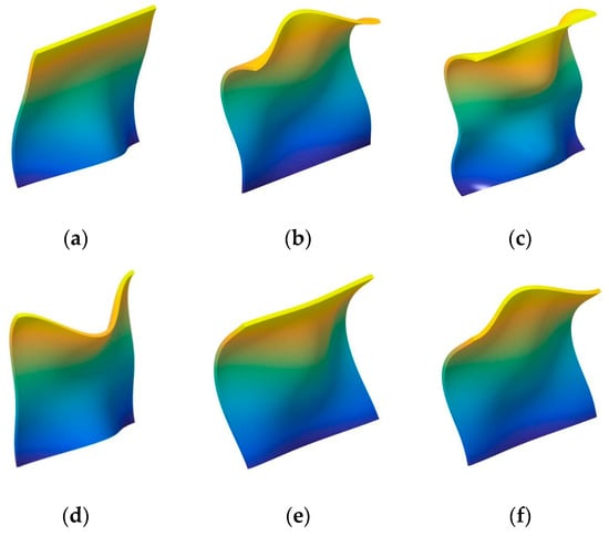
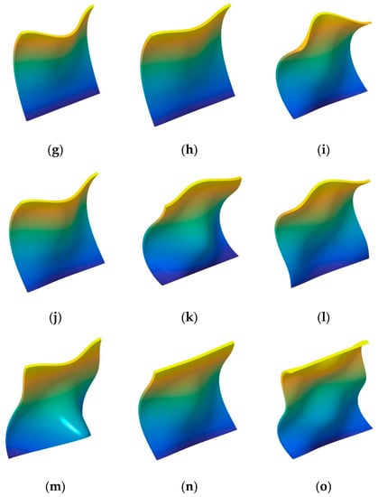
Figure 2.
The mode shapes for the composite laminated shallow cylindrical shell with various boundary conditions. (a) C-C,(1,1); (b) C-C,(1,2); (c) C-C,(1,3); (d) F-C,(1,1); (e) F-C,(1,2); (f) F-C,(1,3); (g) F-F,(1,1); (h) F-F,(1,2); (i) F-F,(1,3); (j) F-S,(1,1); (k) F-S,(1,2); (l) F-S,(1,3); (m) S-C,(1,1); (n) S-C,(1,2); (o) S-C,(1,3).
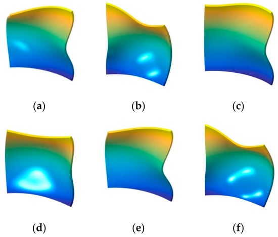
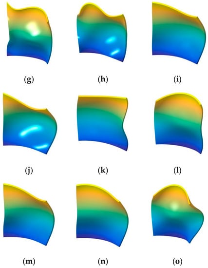
Figure 3.
The mode shapes for the composite laminated shallow spherical shell with various boundary conditions. (a) C-C,(1,1); (b) C-C,(1,2); (c) C-C,(1,3); (d) F-C,(1,1); (e) F-C,(1,2); (f) F-C,(1,3); (g) F-F,(1,1); (h) F-F,(1,2); (i) F-F,(1,3); (j) F-S,(1,1); (k) F-S,(1,2); (l) F-S,(1,3); (m) S-C,(1,1); (n) S-C,(1,2); (o) S-C,(1,3).
In this section, the influence of the length to thickness ratio Lx/h and length to radius ratio Lx/Rx on the fundamental frequency parameter Ω is discussed. In Table 7, Table 8 and Table 9, the fundamental frequency parameter Ω for three types of the layered (i.e., [0°/90°/90°/0°], [0°/90°], and [90°/0°]) composite laminated shallow cylindrical shell, spherical shell, and hyperbolic paraboloidal shell with SD-SD by FSDT and CST is discussed. The material parameters and geometric constants are defined as follows: Lx = 1 m, Ly/Lx = 1, E2 = 7 GPa, E1/E2 = 15, G12 = G13 = 0.5E2, G23 = 0.5E2, μ12 = 0.25, ρ = 1650 kg/m3. Especially with the composite laminated shallow shells with Lx/Rx = 0, the composite shells are transformed into the plate form. From Table 7, Table 8 and Table 9, with the growing of length to radius ratio Lx/Rx (i.e., Lx/Rx = 0, 0.1, 0.2, and 0.5), the fundamental frequency parameters of the composite cylindrical and spherical shell generally grow for various length to thickness ratios Lx/h, lamination schemes, and shell theories. Simultaneously, the fundamental frequency parameters of the composite laminated hyperbolic paraboloidal shell are generally decreased with the changing of the length to radius ratio Lx/Rx. It can be clearly seen that, for different laminated schemes and shell theories, when the length to thickness ratio Lx/h = 0.01, the fundamental frequency parameter of various composite laminated shallow shells increases significantly. Relatively, when Lx/h = 0.1, the frequency parameter increases a little and remains within a stable range. To further investigate the effect of the length to thickness ratio Lx/h on frequency parameters Ω of the composite shallow shell, the variations of the frequency parameter Ω for composite shells with SD-SD boundary conditions, with respect to diverse length to radius ratios Lx/Rx and length to radius ratios Lx/h, by FSDT and CST are shown in Figure 4 and Figure 5. It can be seen that, for different laminated schemes, shallow shell structures, and shell theories, as the length to thickness ratio Lx/h increases, the fundamental frequency parameters Ω gradually decrease. At the same time, it can be seen that, for the composite laminated hyperbolic paraboloidal shell, the variation of the fundamental frequency parameters Ω is small and the effect of the length to thickness ratio Lx/h is not particularly obvious.
Table 7.
The fundamental frequency parameter Ω for three types of layered composite shallow cylindrical shells for variety theories, length to thickness ratios Lx/h, and length to radius ratios Lx/Rx with the SD-SD boundary condition.
Table 8.
The fundamental frequency parameter Ω for three types of layered composite shallow spherical shells for variety theories, length to thickness ratios Lx/h, and length to radius ratios Lx/Rx with the SD-SD boundary condition.
Table 9.
The fundamental frequency parameter Ω for three types of layered composite shallow hyperbolic paraboloidal shells for variety theories, length to thickness ratios Lx/h, and length to radius ratios Lx/Rx with the SD-SD boundary condition.
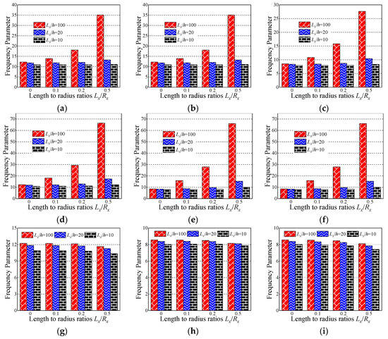
Figure 4.
Variation laws of the fundamental frequency parameter Ω for composite laminated shallow shells with the SD-SD boundary condition with respect to various length to radius ratios Lx/Rx and length to thickness ratios Lx/h by first-order shear deformation shell theory (FSDT). (a) Cylindrical shell, 0°/90°/90°/0°; (b) cylindrical shell, 0°/90°; (c) cylindrical shell, 90°/0°; (d) spherical shell, 0°/90°/90°/0°; (e) spherical shell, 0°/90°; (f) spherical shell, 90°/0°; (g) hyperbolic paraboloidal, 0°/90°/90°/0°; (h) hyperbolic paraboloidal, 0°/90°; (i) hyperbolic paraboloidal, 90°/0°.
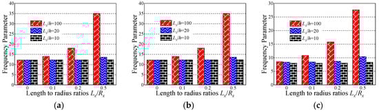
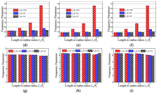
Figure 5.
Variation laws of the fundamental frequency parameter Ω for composite laminated shallow shells with the SD-SD boundary conditions with respect to various length to radius ratios Lx/Rx and length to thickness ratios Lx/h by classical shell theory (CST). (a) Cylindrical shell, 0°/90°/90°/0°; (b) cylindrical shell, 0°/90°; (c) cylindrical shell, 90°/0°; (d) spherical shell, 0°/90°/90°/0°; (e) spherical shell, 0°/90°; (f) spherical shell, 90°/0°; (g) hyperbolic paraboloidal, 0°/90°/90°/0°; (h) hyperbolic paraboloidal, 0°/90°; (i) hyperbolic paraboloidal, 90°/0°.
In the previous numerical example, the effect of geometric parameters on the fundamental frequency parameters is discussed. In this part, the influence of the material parameter on the frequency parameter is investigated. In Table 10 and Table 11, the fundamental frequency parameter for composite laminated shallow spherical shells with various length to radius ratios Lx/Rx, modulus ratios E1/E2, and boundary conditions (i.e., SD-SD, F-F, and C-C) are discussed by FSDT and CST. The material parameters and geometric constants are given as follows: Lx = 1 m, Ly/Lx = 1, h/Ly = 0.1, E2 = 7 GPa, G12 = G13 = 0.5E2, G23 = 0.5E2, μ12 = 0.25, ρ = 1650 kg/m3. It can be clearly seen from Table 10 and Table 11 that the fundamental frequency parameter Ω generally grows with the changing of modulus ratios E1/E2 from 5 to 40. To further reflect the impact of modulus ratios E1/E2 on fundamental frequency parameters, the variations of the fundamental frequency parameter Ω for composite spherical shells with various boundary conditions with respect to multiple length to radius ratios Lx/Rx and modulus ratios E1/E2 by FSDT and CST are shown in Figure 6. Therefore, it can be concluded that the modulus ratios E1/E2 has a significant effect on the fundamental frequency parameters of the composite spherical shell and plays a positive role. Different boundary conditions cause the stiffness matrix to change. For the free boundary condition, the determinant of the stiffness matrix increases with respect to the clamped boundary condition, and when the mass matrix remains unchanged, the natural frequency increases.
Table 10.
The fundamental frequency parameter Ω for composite shallow [0°/90°] spherical shells for variety length to radius ratios Lx/Rx, modulus ratios E1/E2, and boundary conditions by FSDT.
Table 11.
The fundamental frequency parameter Ω for composite shallow [0°/90°] spherical shells for variety length to radius ratios Lx/Rx, modulus ratios E1/E2, and boundary conditions by CST.
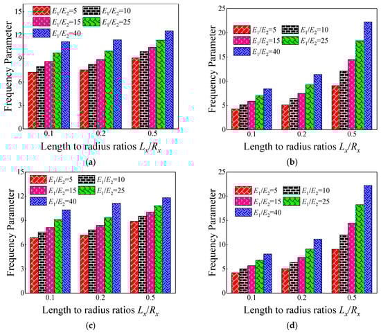
Figure 6.
Variation laws of the fundamental frequency parameter Ω for composite laminated shallow spherical shells with various boundary conditions with respect to diverse length to radius ratios Lx/Rx and modulus ratios E1/E2 by FSDT and CST. (a) FSDT: SD-SD; (b) FSDT: C-C; (c) CST: SD-SD; (d) CST: C-C.
3.2. Composite Laminated Shallow Shell with Elastic Boundary Conditions
The composite laminated shallow shell with elastic constraint is widely encountered in many engineering applications. So, analysis of the composite shallow shells with such an elastic boundary condition is necessary and significant. Therefore, in this section, the free vibration characteristics of the composite shallow shell with elastic boundary conditions are discussed.
In this section, the effect of the restrained springs on the frequency parameter of the certain cross-ply composite laminated shallow shells is discussed. The certain cross-ply layered [0°/90°] composite laminated shallow shells with S-elastic boundary conditions are concerned by FSDT. For the elastic restrained edge, there is only one set of spring component on one displacement or transverse rotational direction and the range of stiffness constants is defined as 100–1012. The material parameters and geometric constants are defined as follows: Lx = 1 m, Ly/Lx = 1, Rx/Ly, E2 = 7 GPa, E1/E2 = 25, G12 = G13 = 0.5E2, G23 = 0.2E2, μ12 = 0.25, ρ = 1650 kg/m3. In Table 12, Table 13, Table 14, Table 15 and Table 16, the lowest two frequency parameter Ω for the composite shells with S-elastic boundary conditions by restrained spring components Ku, Kv, Kw, Kϕx, and Kϕy for a certain circumferential number of n = 1 is calculated.
Table 12.
The frequency parameter Ω for composite shallow [0°/90°] shells with S-Ku boundary conditions by FSDT.
Table 13.
The frequency parameter Ω for composite shallow [0°/90°] shells with S-Kv boundary conditions by FSDT.
Table 14.
The frequency parameter Ω for composite shallow [0°/90°] shells with S-Kw boundary conditions by FSDT.
Table 15.
The frequency parameter Ω for composite shallow [0°/90°] shells with S-Kϕx boundary conditions by FSDT.
Table 16.
The frequency parameter Ω for composite shallow [0°/90°] shells with S-Kϕy boundary conditions by FSDT.
In Table 12 and Table 13, when the certain cross-ply composite laminated shallow shells are only restrained in the direction of u and v, the frequency parameters generally increase with the various composite laminated shallow shell forms. Also, the increase in frequency parameters is small and basically remains within a stable range. Correspondingly, when Ku = 106, the frequency parameter starts to increase slightly, and when Ku = 1010, the frequency parameter remains basically unchanged. When the composite laminated shallow shells are under the elastic restraint Kw in Table 14, the frequency parameters Ω are generally decreased with the growing of the spring stiffness from 100 to 1012. In particular, for the hyperbolic paraboloidal shell, the frequency parameter increases less than that of the other composite laminated shallow shell forms. For the effect of transverse rotational spring stiffness on the frequency parameter of composite laminated shallow shells, Table 15 and Table 16 show the changing rule of the frequency parameters with the growing of the stiffness constants for Kϕx and Kϕy. In general, as the stiffness constants Kϕx and Kϕy continue to increase, the frequency parameters corresponding to each structure tend to increase; at the same time, the main change region of the frequency parameter is between Kϕx,y = 104–1010. However, when Kϕx,y = 107, there will be some jitter in the frequency parameters, which suddenly increase or decrease. Therefore, as the elastic restrained stiffness constants in different directions increase, the frequency parameters of various composite shell forms are gradually increasing and have different change regions. Furthermore, the variations of the frequency parameter with the changing of the stiffness constants are shown in Figure 7, Figure 8, Figure 9, Figure 10 and Figure 11.
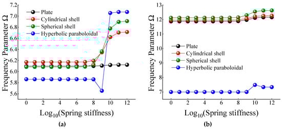
Figure 7.
Variation laws of the frequency parameter Ω for composite shallow [0°/90°] shells with various stiffness constant Ku by FSDT. (a) m = 1; (b) m = 2.
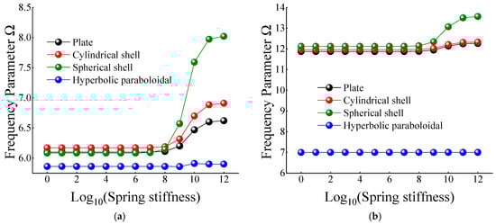
Figure 8.
Variation laws of the frequency parameter Ω for composite shallow [0°/90°] shells with various stiffness constant Kv by FSDT. (a) m = 1; (b) m = 2.
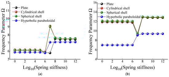
Figure 9.
Variation laws of the frequency parameter Ω for composite shallow [0°/90°] shells with various stiffness constant Kw by FSDT. (a) m = 1; (b) m = 2.
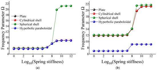
Figure 10.
Variation laws of the frequency parameter Ω for composite shallow [0°/90°] shells with various stiffness constant Kϕx by FSDT. (a) m = 1; (b) m = 2.
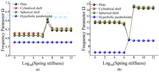
Figure 11.
Variation laws of the frequency parameter Ω for composite shallow [0°/90°] shells with various stiffness constant Kϕy by FSDT. (a) m = 1; (b) m = 2.
4. Conclusions
A semi-analyzed method is conducted for the free vibration characteristics of composite laminated shallow shells with general boundary conditions, including classical boundary conditions, elastic boundary conditions, and their combinations. Through the relationship between the displacement vector and force resultants, the formulations are established related to classical shell theory (CST) and first-order shear deformation shell theory (FSDT). According to diverse boundary conditions, the boundary matrix and the total matrix of the composite shallow shell will be established. Through the dichotomy method to search the zeros position of the total matrix determinant, the natural frequency can be obtained. Correspondingly, some numerical examples are calculated and the conclusions can be summarized as follows:
First, by comparing the solutions by the presented method with some reported literature results, the correctness of the calculation for the free vibration characteristics of composite laminated shallow shells with classical boundary conditions, elastic boundary conditions, and their combinations can be proven.
Second, some numerical examples are extended to investigate the influence of material parameters and geometric constants, like length to radius ratios, length to thickness ratios, and modulus ratios, on the frequency parameter. It can concluded that different material and geometric parameters have different influence factors on frequency parameters. Simultaneously, changing laws obtained by various composite laminated shallow shell structures are not consistent.
Finally, the effect of boundary elastic restrained stiffness on the natural frequency parameters is discussed. By changing the value of the spring stiffness in different displacement directions and transverse rotation from 100 to 1012, the variation of the frequency parameter with the elastic restrained spring stiffness constants is obtained. It can be seen from numerical analysis examples that the different elastic constants have a positive effect on the frequency parameters and have a certain effect on the increase of the frequency parameters. Simultaneously, the effect of each spring stiffness constant has its own influence range.
Author Contributions
Methodology, D.S.; validation, D.H. and Q.W.; formal analysis, D.H.; investigation, D.H. and Q.W.; data curation, D.H. and Q.W.; writing—original draft preparation, D.H. and C.M.; writing—review and editing, Q.W. visualization, D.H.; supervision, D.S. and H.S.
Funding
This research was funded by the National Natural Science Foundation of China (Grant Nos. 51679056, 51705537 and 51875112), Innovation Driven Program of Central South University (Grant number: 2019CX006), and the Natural Science Foundation of Hunan Province of China (2018JJ3661). The authors also gratefully acknowledge the supports from State Key Laboratory of High Performance Complex Manufacturing, Central South University, China (Grant No. ZZYJKT2018-11).
Conflicts of Interest
The authors declare no conflict of interest.
References
- Qatu, M.S.; Sullivan, R.W.; Wang, W. Recent research advances on the dynamic analysis of composite shells: 2000–2009. Compos. Struct. 2010, 93, 14–31. [Google Scholar] [CrossRef]
- Qatu, M.S. Resent research advances in the dynamic behavior of shells: 1989–2000, Part 1: Laminated composite shells. Appl. Mech. Rev. 2002, 55, 325–350. [Google Scholar] [CrossRef]
- Leissa, A.W.; Nordgren, R.P. Vibration of Shells. J. Appl. Mech. 1973, 41, 544. [Google Scholar] [CrossRef]
- Reddy, J. Energy and Variational Methods in Applied Mechanics; John Willey & Sons: New York, NY, USA, 1984. [Google Scholar]
- Reissner, E.; Wan, F. A note on the linear theory of shallow shear-deformable shells. Z. Angew. Math. Phys. ZAMP 1982, 33, 425–427. [Google Scholar] [CrossRef]
- Neves, A.M.A.; Ferreira, A.J.M.; Carrera, E.; Cinefra, M.; Roque, C.M.C.; Jorge, R.M.N.; Soares, C.M.M. Free vibration analysis of functionally graded shells by a higher-order shear deformation theory and radial basis functions collocation, accounting for through-the-thickness deformations. Eur. J. Mech. A Solids 2013, 37, 24–34. [Google Scholar] [CrossRef]
- Viola, E.; Tornabene, F.; Fantuzzi, N. General higher-order shear deformation theories for the free vibration analysis of completely doubly-curved laminated shells and panels. Compos. Struct. 2013, 95, 639–666. [Google Scholar] [CrossRef]
- Reddy, J.N.; Liu, C.F. A higher-order shear deformation theory of laminated elastic shells. Int. J. Eng. Sci. 1985, 23, 319–330. [Google Scholar] [CrossRef]
- Tsai, C.T.; Palazotto, A.N. A modified riks approach to composite shell snapping using a high-order shear deformation theory. Comput. Struct. 1990, 35, 221–226. [Google Scholar] [CrossRef]
- Viola, E.; Tornabene, F.; Fantuzzi, N. Static analysis of completely doubly-curved laminated shells and panels using general higher-order shear deformation theories. Compos. Struct. 2013, 101, 59–93. [Google Scholar] [CrossRef]
- Reddy, J.N. Mechanics of Laminated Composite Plates and Shells: Theory and Analysis; CRC Press: Boca Raton, FL, USA, 2003. [Google Scholar]
- Leissa, A.W. Vibration of Shells; NASA-SP-288, LC-77-186367; NASA: Washington, DC, USA, 1 January 1973.
- Qatu, M.S. Vibration of Laminated Shells and Plates; Elsevier: Amsterdam, The Netherlands, 2004. [Google Scholar]
- Ye, T.; Jin, G.; Chen, Y.; Ma, X.; Zhu, S. Free vibration analysis of laminated composite shallow shells with general elastic boundaries. Compos. Struct. 2013, 106, 470–490. [Google Scholar] [CrossRef]
- Kurpa, L.; Shmatko, T.; Timchenko, G. Free vibration analysis of laminated shallow shells with complex shape using the -functions method. Compos. Struct. 2010, 93, 225–233. [Google Scholar] [CrossRef]
- Fazzolari, F.A.; Carrera, E. Advances in the Ritz formulation for free vibration response of doubly-curved anisotropic laminated composite shallow and deep shells. Compos. Struct. 2013, 101, 111–128. [Google Scholar] [CrossRef]
- Awrejcewicz, J.; Kurpa, L.; Osetrov, A. Investigation of the stress-strain state of the laminated shallow shells by R-functions method combined with spline-approximation. ZAMM J. Appl. Math. Mech. 2011, 91, 458–467. [Google Scholar] [CrossRef]
- Tran, M.T.; Nguyen, V.L.; Trinh, A.T. Static and vibration analysis of cross-ply laminated composite doubly curved shallow shell panels with stiffeners resting on Winkler–Pasternak elastic foundations. Int. J. Adv. Struct. Eng. 2017, 9, 153–164. [Google Scholar] [CrossRef][Green Version]
- Biswal, M.; Sahu, S.K.; Asha, A.V. Experimental and numerical studies on free vibration of laminated composite shallow shells in hygrothermal environment. Compos. Struct. 2015, 127, 165–174. [Google Scholar] [CrossRef]
- Garcia, C.; Trendafilova, I.; Zucchelli, A. The effect of polycaprolactone nanofibers on the dynamic and impact behavior of glass fibre reinforced polymer composites. J. Compos. Sci. 2018, 2, 43. [Google Scholar] [CrossRef]
- Garcia, C.; Wilson, J.; Trendafilova, I.; Yang, L. Vibratory behaviour of glass fibre reinforced polymer (GFRP) interleaved with nylon nanofibers. Compos. Struct. 2017, 176, 923–932. [Google Scholar] [CrossRef]
- Shao, D.; Hu, S.; Wang, Q.; Pang, F. An enhanced reverberation-ray matrix approach for transient response analysis of composite laminated shallow shells with general boundary conditions. Compos. Struct. 2017, 162, 133–155. [Google Scholar] [CrossRef]
- Leissa, A.W.; Qatu, M.S. Equations of Elastic Deformation of Laminated Composite Shallow Shells. J. Appl. Mech. 1991, 58, 1497–1500. [Google Scholar] [CrossRef]
- Qatu, M.S.; Leissa, A.W. Free vibrations of completely free doubly curved laminated composite shallow shells. J. Sound Vib. 1991, 151, 9–29. [Google Scholar] [CrossRef]
- Lim, C.W.; Liew, K.M. A higher order theory for vibration of shear deformable cylindrical shallow shells. Int. J. Mech. Sci. 1995, 37, 277–295. [Google Scholar] [CrossRef]
- Barai, A.; Durvasula, S. Vibration and buckling of hybrid laminated curved panels. Compos. Struct. 1992, 21, 15–27. [Google Scholar] [CrossRef]
- Leissa, A.W.; Narita, Y. Vibrations of completely free shallow shells of rectangular planform. J. Sound Vib. 1984, 96, 207–218. [Google Scholar] [CrossRef]
- Fazzolari, F.A. A refined dynamic stiffness element for free vibration analysis of cross-ply laminated composite cylindrical and spherical shallow shells. Compos. Part B Eng. 2014, 62, 143–158. [Google Scholar] [CrossRef]
- Bhimaraddi, A. Free vibration analysis of doubly curved shallow shells on rectangular planform using three-dimensional elasticity theory. Int. J. Solids Struct. 1991, 27, 897–913. [Google Scholar] [CrossRef]
- Librescu, L.; Khdeir, A.A.; Frederick, D. A shear deformable theory of laminated composite shallow shell-type panels and their response analysis I: Free vibration and buckling. Acta Mech. 1989, 76, 1–33. [Google Scholar] [CrossRef]
- Bhimaraddi, A. Three-dimensional elasticity solution for static response of orthotropic doubly curved shallow shells on rectangular planform. Compos. Struct. 1993, 24, 67–77. [Google Scholar] [CrossRef]
- Wang, J.; Schweizerhof, K. Study on free vibration of moderately thick orthotropic laminated shallow shells by boundary-domain elements. Appl. Math. Model. 1996, 20, 579–584. [Google Scholar] [CrossRef]
- Zhao, X.; Liew, K.M.; Ng, T.Y. Vibration analysis of laminated composite cylindrical panels via a meshfree approach. Int. J. Solids Struct. 2003, 40, 161–180. [Google Scholar] [CrossRef]
- Dennis, S.T. A Galerkin solution to geometrically nonlinear laminated shallow shell equations. Comput. Struct. 1997, 63, 859–874. [Google Scholar] [CrossRef]
- Kobayashi, Y. Large amplitude free vibration of thick shallow shells supported by shear diaphragms. Int. J. Non-Linear Mech. 1995, 30, 57–66. [Google Scholar] [CrossRef]
- Chakravorty, D.; Bandyopadhyay, J.N.; Sinha, P.K. Finite element free vibration analysis of doubly curved laminated composite shells. J. Reinf. Plast. Compos. 1996, 15, 322–342. [Google Scholar] [CrossRef]
- Beakou, A.; Touratier, M. A rectangular finite element for analysis composite multilayerd shallow shells in static, vibration and buckling. Int. J. Numer. Methods Eng. 2010, 36, 627–653. [Google Scholar] [CrossRef]
- Mahapatra, T.R.; Panda, S.K. Thermoelastic Vibration Analysis of Laminated Doubly Curved Shallow Panels Using Non-Linear FEM. J. Therm. Stresses 2015, 38, 39–68. [Google Scholar] [CrossRef]
- Desmet, W. A Wave Based Prediction Technique for Coupled Vibro-Acoustic Analysis. Ph.D. Thesis, Katholieke Universiteit Leuven, Leuven, Belgium, 1998. [Google Scholar]
- Deckers, E.; Atak, O.; Coox, L.; D’Amico, R.; Devriendt, H.; Jonckheere, S.; Koo, K.; Pluymers, B.; Vandepitte, D.; Desmet, W. The wave based method: An overview of 15years of research. Wave Motion 2014, 51, 550–565. [Google Scholar] [CrossRef]
- Chen, M.; Xie, K.; Xu, K.; Yu, P. Wave Based Method for Free and Forced Vibration Analysis of Cylindrical Shells with Discontinuity in Thickness. J. Vib. Acoust. 2015, 137, 051004. [Google Scholar] [CrossRef]
- Xie, K.; Chen, M.; Deng, N.; Xu, K. Wave based method for vibration and acoustic characteristics analysis of underwater cylindrical shell with bulkheads. In Proceedings of the INTER-NOISE and NOISE-CON Congress and Conference, Melbourne, Australia, 16–19 November 2014. [Google Scholar]
- Wei, J.; Chen, M.; Hou, G.; Xie, K.; Deng, N. Wave Based Method for Free Vibration Analysis of Cylindrical Shells with Nonuniform Stiffener Distribution. J. Vib. Acoust. 2013, 135, 061011. [Google Scholar] [CrossRef]
- Chen, W.; Wei, J.; Xie, K.; Deng, N.; Hou, G. Wave based method for free vibration analysis of ring stiffened cylindrical shell with intermediate large frame ribs. Shock Vib. 2013, 20, 459–479. [Google Scholar] [CrossRef]
- Xie, K.; Chen, M.; Zhang, L.; Xie, D. Wave based method for vibration analysis of elastically coupled annular plate and cylindrical shell structures. Appl. Acoust. 2017, 123, 107–122. [Google Scholar] [CrossRef]
- He, D.; Shi, D.; Wang, Q.; Shuai, C. Wave based method (WBM) for free vibration analysis of cross-ply composite laminated cylindrical shells with arbitrary boundaries. Compos. Struct. 2019, 213, 284–298. [Google Scholar] [CrossRef]
© 2019 by the authors. Licensee MDPI, Basel, Switzerland. This article is an open access article distributed under the terms and conditions of the Creative Commons Attribution (CC BY) license (http://creativecommons.org/licenses/by/4.0/).