Non-Deterministic Assessment of Surface Roughness as Bond Strength Parameters between Concrete Layers Cast at Different Ages

 , , , and
Abstract
:1. Introduction
- It requires standardisation due to its importance in practice.
- Aggressive contaminants may penetrate the delaminated interface and cause unfavourable conditions for durability.
- Element stiffness may be reduced and larger deformations appear, reducing serviceability.
- Load transfer between layers changes with the bond failure.
- Shrinkage is a factor that influences pure cohesive action and element deformations.
- Cohesion, due to mechanical interlocking between particles;
- Friction, due to the existence of compression stresses at the interface and due to the relative displacement between concrete parts;
- Dowel action, due to the deformation of the reinforcement bars crossing the interface.
- More detailed investigation—both roughness and waviness are considered, so profile height and inclination variability are identified.
- Application of random surfaces, i.e., storing information on surface texture in a random image of a real surface.
- Introduction of statistical objective parameters instead of traditional roughness parameters in order to reproduce the randomness of any surface texture.
2. Materials and Methods
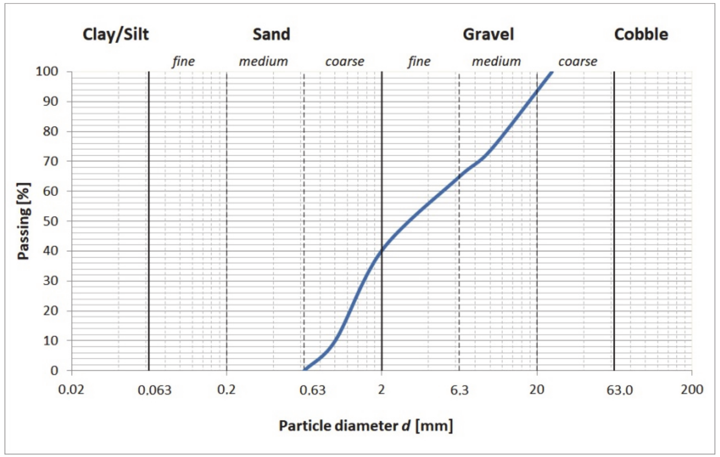
2.1. Concrete Mix Composition
2.2. Samples
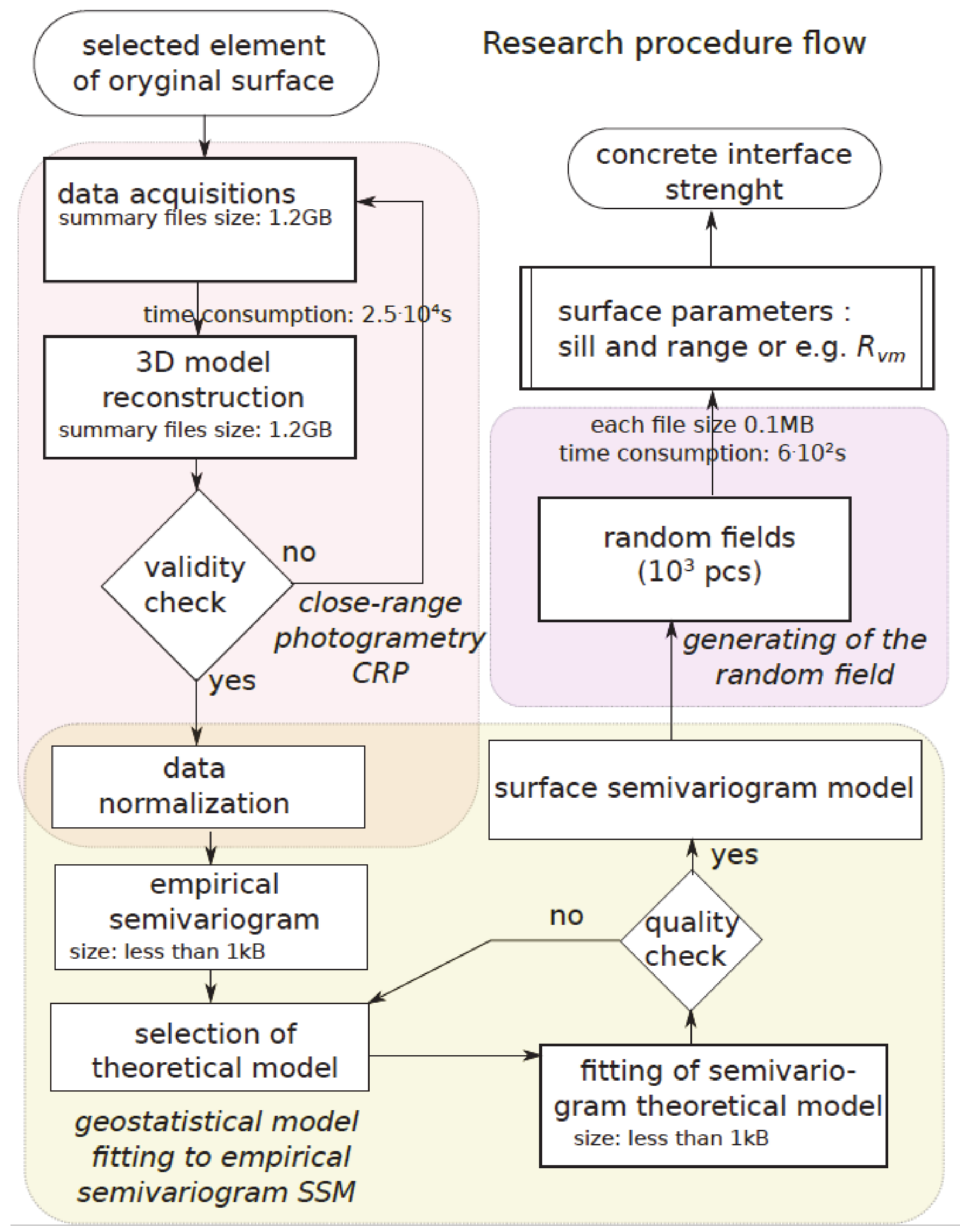
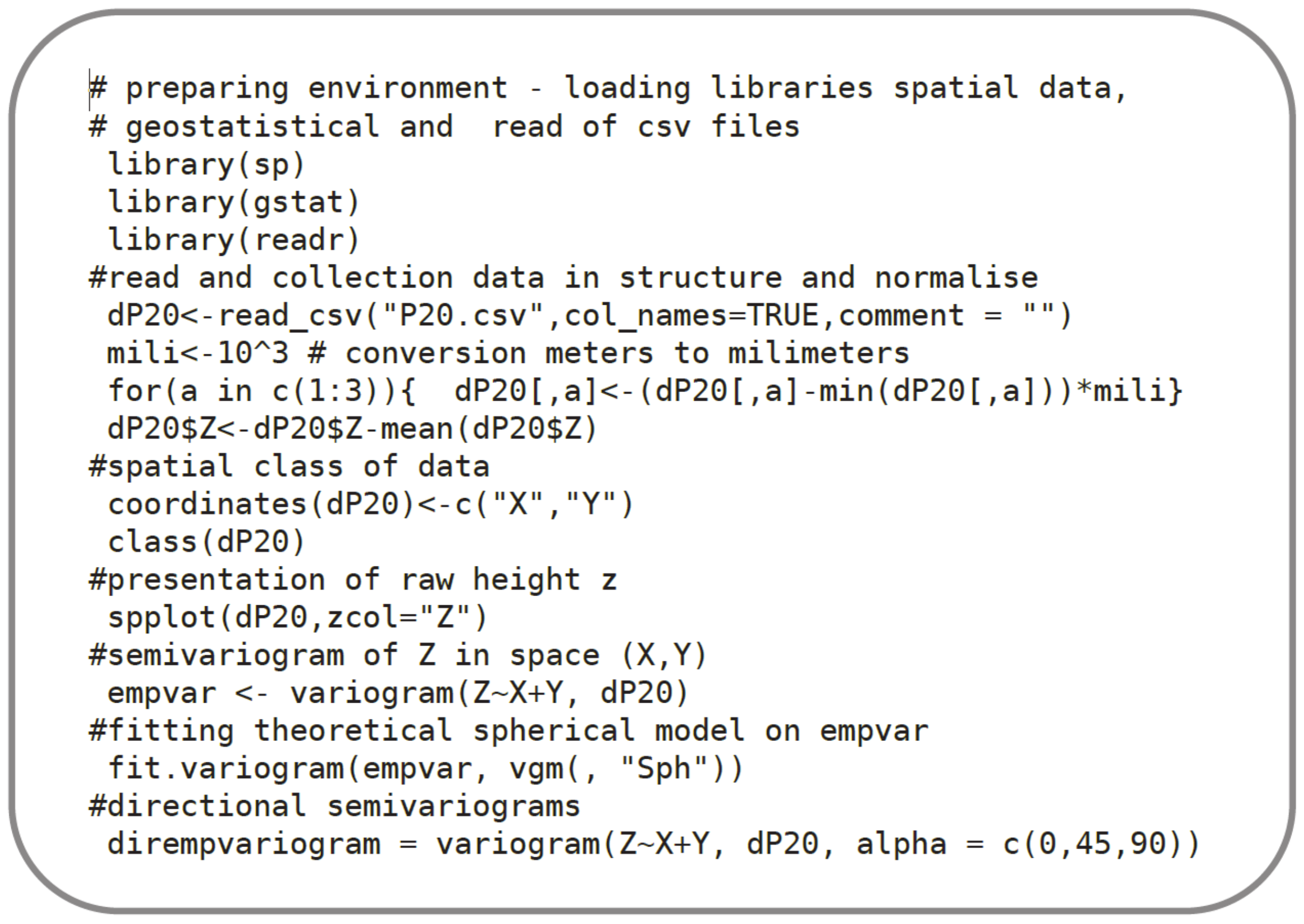
2.3. Background of the Proposed Method
- point cloud acquisition (with known coordinates (x,y,z) representing sample surface) with an adequate accuracy;
- surface assessment with use of geostatistical methods, i.e., fitting of theoretical semivariogram to empirical data;
- generation of Gaussian random field (via height profiles) based on the fitted semivariogram;
- computation of the roughness/texture parameters based on the generated profiles or surfaces;
- correlation analysis of the semivariogram parameters with shear strength factors throughout roughness/texture parameters.
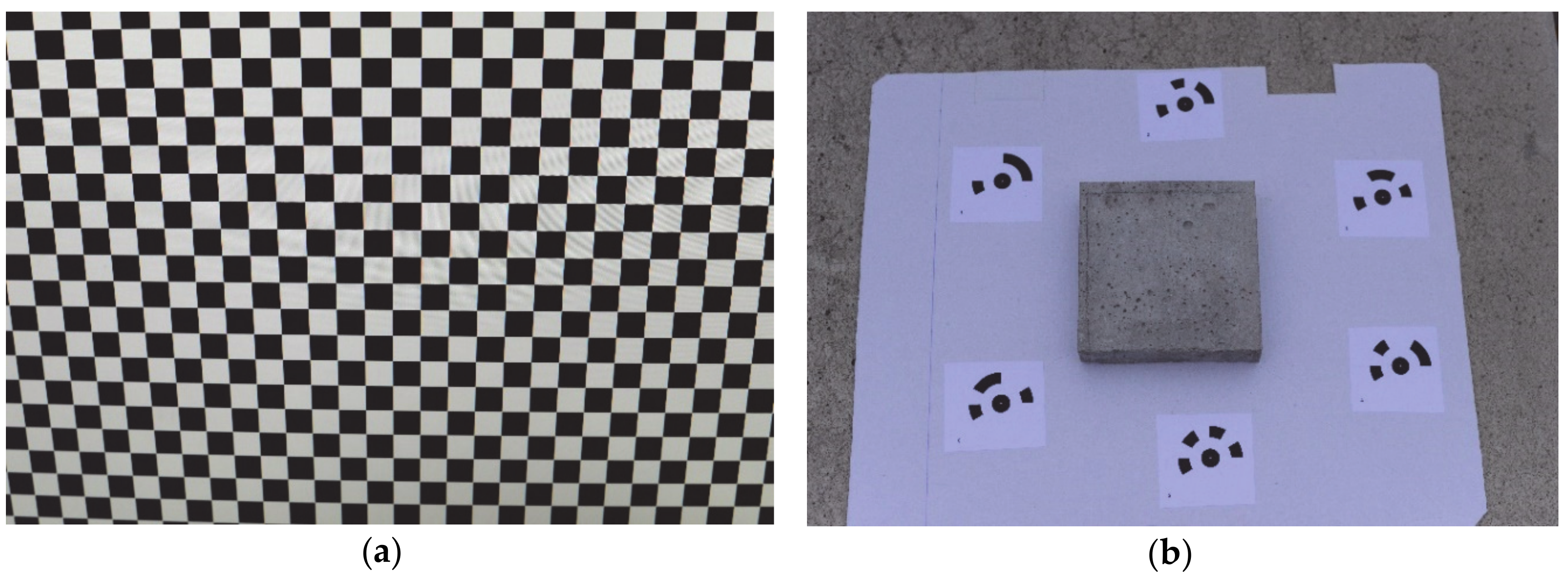
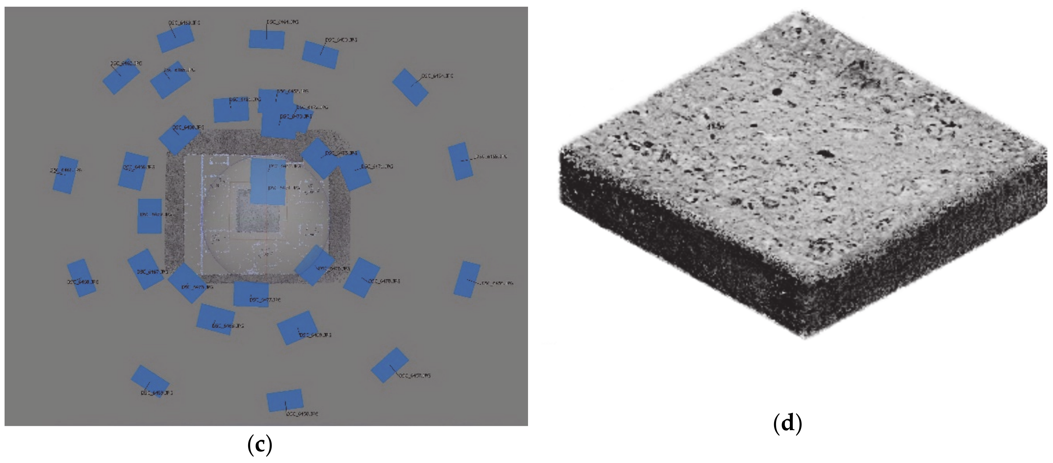
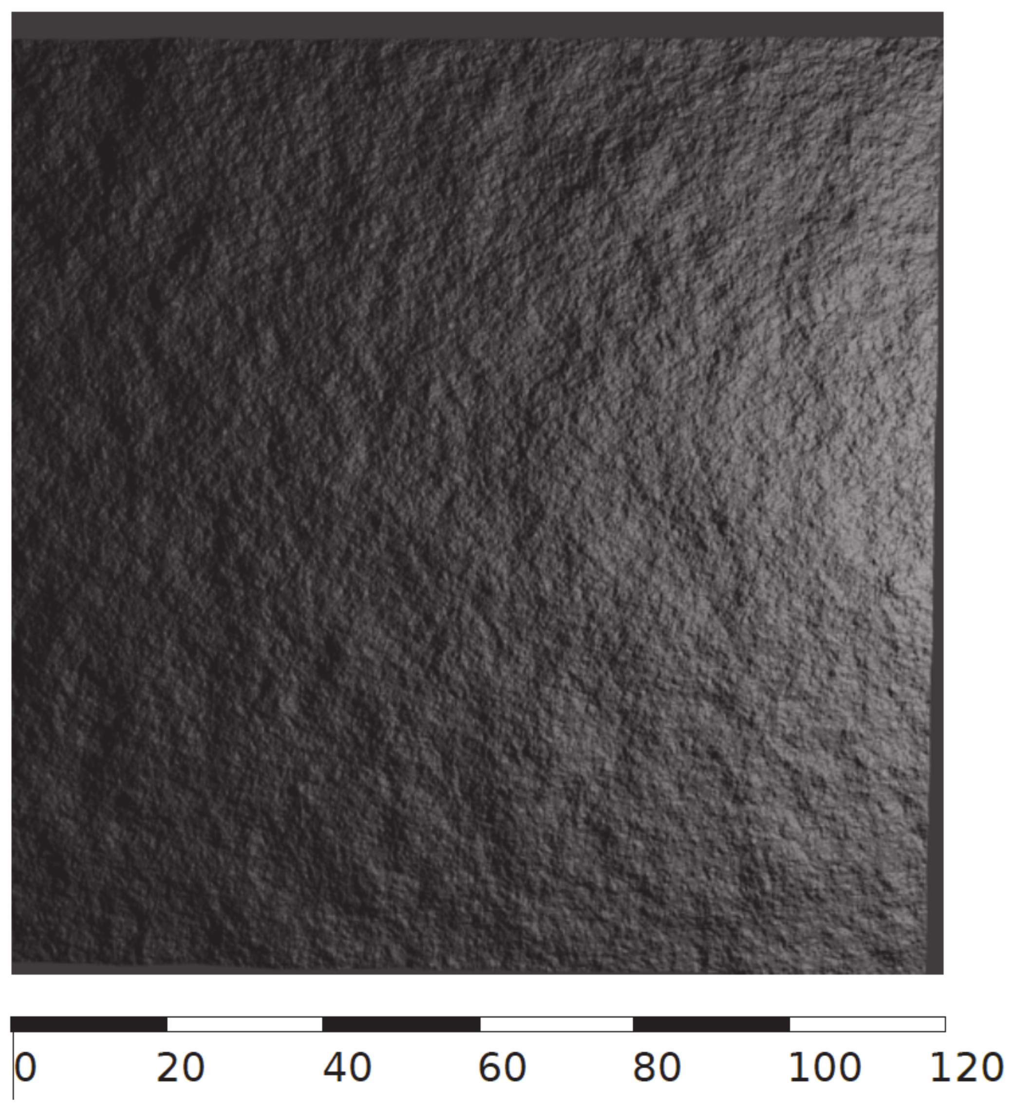
2.4. Data Acquisition Employing Photogrammetry
2.5. Geostatistical Models of the Sample Surfaces
- The distance where the model first flattens is known as the range r [L].
- Point or sample locations separated by a distance smaller than the range r are spatially autocorrelated, whereas locations farther apart than the range r are not.
- The value that the semivariogram model attains at the range r is called the sill s [L2]. The partial sill is the sill minus the nugget [L2].
- Theoretically, at zero separation distance (lag = 0 [L]), the semivariogram value is 0 [L2]. However, at an infinitesimally small separation distance, the semivariogram often exhibits a nugget [L2] effect, which is some value greater than 0. The nugget effect can be attributed to measurement error or spatial sources of variation at distances smaller than the sampling interval, or both. Natural phenomena can vary spatially over a range of scales. Variation at microscales smaller than the sampling distance will appear as part of the nugget effect.
2.6. Geostatistical Model Fitting to Empirical Semivariogram—Surface Semivariogram Model (SSM)
- for each pair of points from the surface,
- for a combination of points along parallel lines in (0°, 45° or 90°).
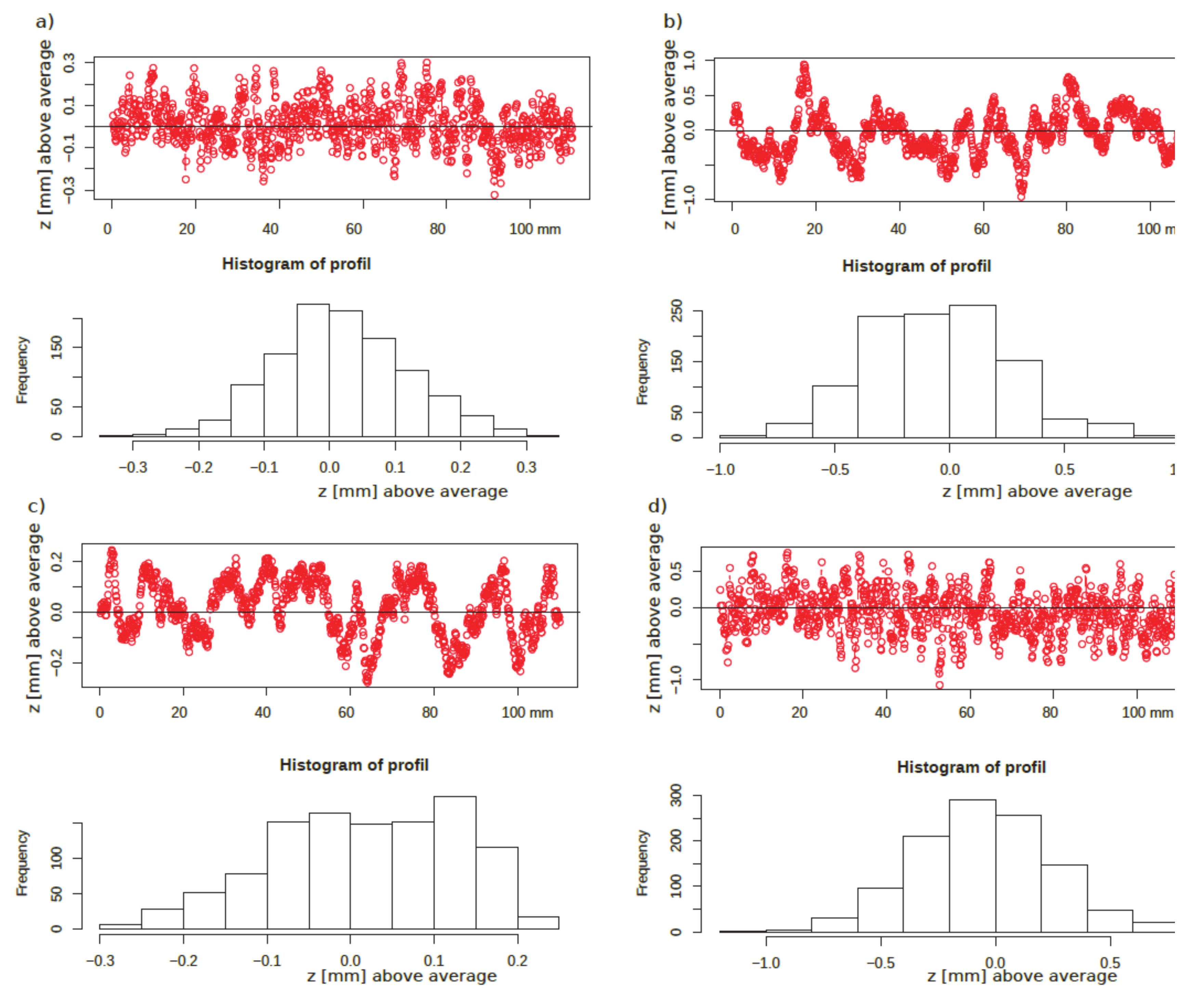
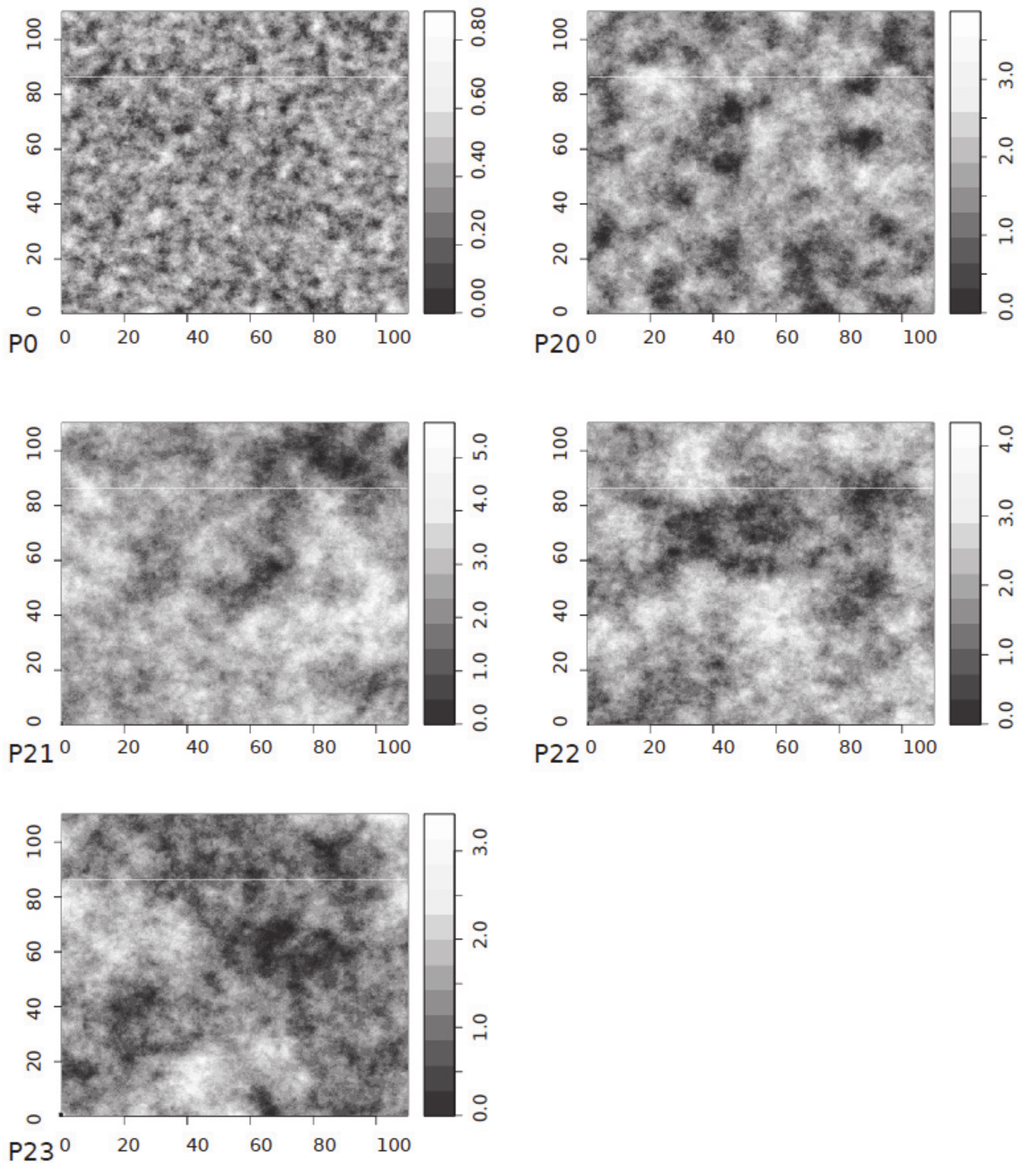
2.7. Generation of the Random Field
2.8. Surface Roughness Parameters
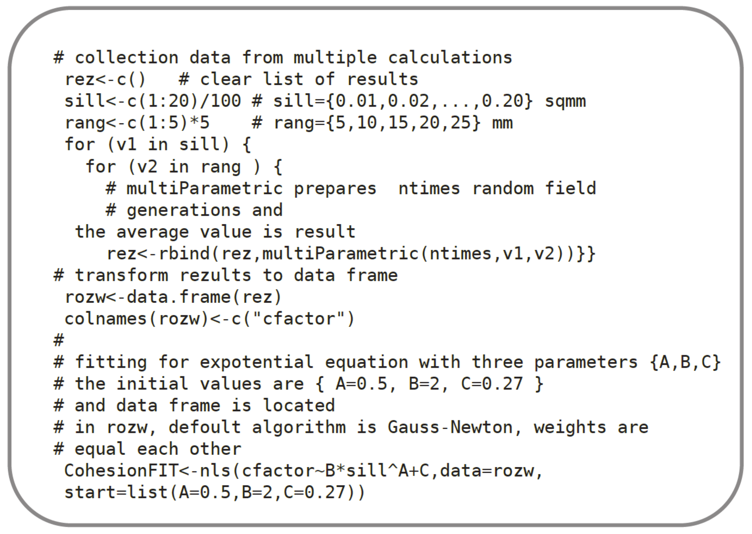
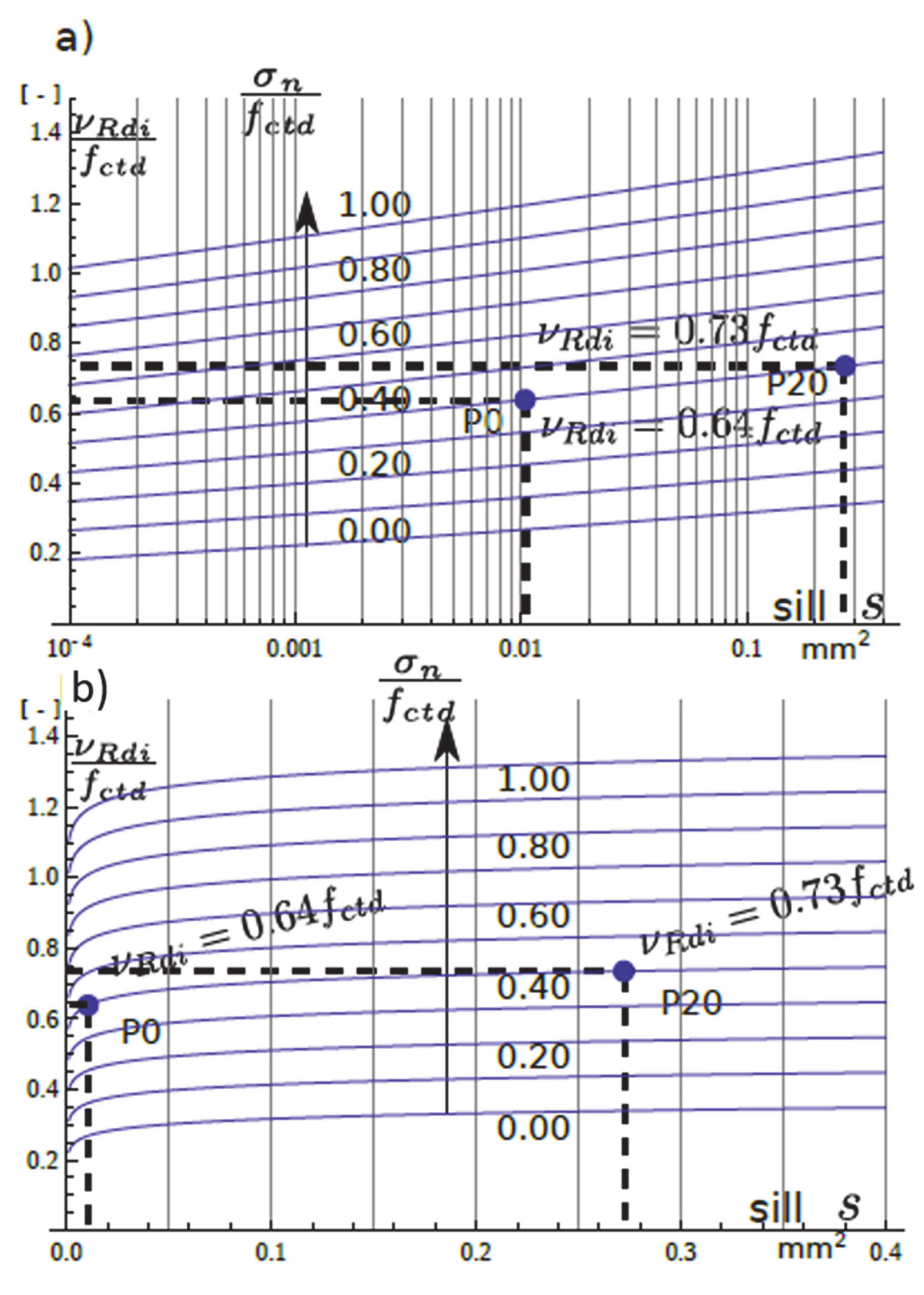
2.9. Concrete Interface Strength
3. Results and Discussion
4. Conclusions
Author Contributions
Funding
Acknowledgments
Conflicts of Interest
References
- Cranston, W.B.; Kamiński, M.; Wróblewski, R. Aggregate interlock in cracked concrete with excessive crack width. Arch. Civ. Eng. 1996, 42, 177–193. [Google Scholar]
- Birkeland, P.W.; Birkeland, H.W. Connections in Precast Concrete Construction. ACI J. Proc. 1966, 63, 345–368. [Google Scholar]
- EN 1992-1-1 Eurocode 2: Design of Concrete Structures -Part 1-1: General Rules and Rules for Buildings; Comité Européen de Normalisation: Brussels, Belgium, 2004.
- Model Code 2010: Final Draft; International Federation for Structural Concrete (fib): Laussane, Switzerland, 2012.
- Santos, P.M.D. Assessment of the Shear Strength between Concrete Layers. In Proceedings of the 8th Fib International PhD Symposium in Civil Engineering, Copenhagem, Denmark, 20–23 June 2010. [Google Scholar]
- Walraven, J.C.; Reinhardt, H.W. Theory and Experiments on the Mechanical Behaviour of Cracks in Plain and Reinforced Concrete Subjected to Shear Loading. HERON 1981, 26, 1–68. [Google Scholar]
- Vecchio, F.J.; Collins, M.P. Modified Compression-Field Theory for Reinforced Concrete Elements Subjected To Shear. J. Am. Concr. Inst. 1986, 83, 219–231. [Google Scholar]
- Santos, P.M.D.; Júlio, E.N.B.S. A state-of-the-art review on roughness quantification methods for concrete surfaces. Constr. Build. Mater. 2013, 38, 912–923. [Google Scholar] [CrossRef]
- Mohamad, M.E.; Ibrahim, I.S.; Abdullah, R.; Abd Rahman, A.B.; Kueh, A.B.H.; Usman, J. Friction and cohesion coefficients of composite concrete-to-concrete bond. Cem. Concr. Compos. 2015, 56, 1–14. [Google Scholar] [CrossRef]
- Santos, P.M.D.; Júlio, E.N.B.S. Interface shear transfer on composite concrete members. ACI Struct. J. 2014, 111, 113–121. [Google Scholar]
- Figueira, D.; Sousa, C.; Calçada, R.; Serra Neves, A. Design recommendations for reinforced concrete interfaces based on statistical and probabilistic methods. Struct. Concr. 2016, 17, 811–823. [Google Scholar] [CrossRef]
- EN 1990. Eurocode–Basis of Structural Design; Comité Européen de Normalisation: Brussels, Belgium, 2005.
- Schabowicz, K.; Ranachowski, Z.; Jóźwiak-Niedźwiedzka, D.; Radzik, Ł.; Kudela, S.; Dvorak, T. Application of X-ray microtomography to quality assessment of fibre cement boards. Constr. Build. Mater. 2016, 110, 182–188. [Google Scholar] [CrossRef]
- Schabowicz, K. Non-destructive testing of materials in civil engineering. Materials 2019, 12, 3237. [Google Scholar] [CrossRef] [Green Version]
- Hoła, J.; Sadowski, Ł.; Reiner, J.; Stach, S. Usefulness of 3D surface roughness parameters for nondestructive evaluation of pull-off adhesion of concrete layers. Constr. Build. Mater. 2015, 84, 111–120. [Google Scholar] [CrossRef]
- Courard, L.; Piotrowski, T.; Garbacz, A. Near-to-surface properties affecting bond strength in concrete repair. Cem. Concr. Compos. 2014, 46, 73–80. [Google Scholar] [CrossRef]
- Sadowski, Ł.; Hoła, J. New nondestructive way of identifying the values of pull-off adhesion between concrete layers in floors. J. Civ. Eng. Manag. 2014, 20, 561–569. [Google Scholar] [CrossRef] [Green Version]
- Trapko, T.; Musiał, M. PBO mesh mobilization via different ways of anchoring PBO-FRCM reinforcements. Compos. Part B Eng. 2017, 118, 67–74. [Google Scholar] [CrossRef]
- Gaetan, C.; Guyon, X. Springer Series in Statistics Spatial Statistics and Modeling; Springer: Berlin/Heidelberg, Germany, 2010. [Google Scholar]
- Wackernagel, H. MultivariateGeostatistics. An Itroduction and Applications; Springer: Berlin/Heidelberg, Germany, 2003. [Google Scholar]
- Diggle, P.J.; Tawn, J.A. Model-based geostatistics. Appl. Stat. 1998, 47, 299–350. [Google Scholar] [CrossRef]
- The R Project for Statistical Computing. Available online: https://www.R-project.org/ (accessed on 20 May 2020).
- EN ISO 14688-2. Geotechnical Investigation and Testing–Identification and Classification of Soil–Part 2: Principles for a Classification; Comité Européen de Normalisation: Brussels, Belgium, 2017.
- EN 933-4. Tests for Geometrical Properties of Aggregates Part 4: Determination of Particle Shapes-Shape Index; Comité Européen de Normalisation: Brussels, Belgium, 2008.
- Arias, P.; Armesto, J.; Di-Capua, D.; González-Drigo, R.; Lorenzo, H.; Pérez-Gracia, V. Digital photogrammetry, GPR and computational analysis of structural damages in a mediaeval bridge. Eng. Fail. Anal. 2007, 14, 1444–1457. [Google Scholar] [CrossRef]
- Psaltis, C.; Ioannidis, C. An automatic technique for accurate non-contact structural deformation measurements. In Proceedings of the International Archives of the Photogrammetry, Remote Sensing and Spatial Information Sciences -ISPRS Archives, Dresden, Germany, 25–27 September 2006. [Google Scholar]
- Kwak, E.; Detchev, I.; Habib, A.; El-Badry, M.; Hughes, C. Precise photogrammetric reconstruction using model-based image fitting for 3D beam deformation monitoring. J. Surv. Eng. 2013, 139, 143–155. [Google Scholar] [CrossRef]
- Baqersad, J.; Poozesh, P.; Niezrecki, C.; Avitabile, P. Photogrammetry and optical methods in structural dynamics–A review. Mech. Syst. Signal Process. 2017, 86, 17–34. [Google Scholar] [CrossRef]
- Farahani, B.V.; Barros, F.; Sousa, P.J.; Cacciari, P.P.; Tavares, P.J.; Futai, M.M.; Moreira, P. A coupled 3D laser scanning and digital image correlation system for geometry acquisition and deformation monitoring of a railway tunnel. Tunn. Undergr. Sp. Technol. 2019, 91, 102995. [Google Scholar] [CrossRef]
- Muszyński, Z.; Rybak, J.; Kaczor, P. Accuracy Assessment of Semi-Automatic Measuring Techniques Applied to Displacement Control in Self-Balanced Pile Capacity Testing Appliance. Sensors 2018, 18, 4067. [Google Scholar] [CrossRef] [Green Version]
- Agisoft Lens. Version 0.4.2 beta 64bit (build 2399). Lens Calibration Software. Agisoft LLC. 2016. Available online: http://www.agisoft.com (accessed on 16 April 2018).
- Agisoft PhotoScan Professional Edition. Version 1.2.4 64 bit (build 2399). Multi-View 3D Reconstruction. Agisoft LLC. 2016. Available online: http://www.agisoft.com (accessed on 16 April 2018).
- Isaaks, E.H.; Srivastava, R.M. An Introduction to Applied Geostatistics; Oxford University Press: New York, NY, USA, 1989. [Google Scholar]
- Pebesma, E.J. Multivariable geostatistics in S: The gstat package. Comput. Geosci. 2004, 30, 683–691. [Google Scholar] [CrossRef]
- Pebesma, E.J.; Wesseling, C.G. Gstat: A program for geostatistical modelling, prediction and simulation. Comput. Geosci. 1998, 24, 17–31. [Google Scholar] [CrossRef]
- Bivand, R.S.; Pebesma, E.; Gómez-Rubio, V. Applied Spatial Data Analysis with R; Springer: Berlin/Heidelberg, Germany, 2013; ISBN 9781461476177. [Google Scholar]
- Clarkson, K.L. Fast algorithms for the all nearest neighbours problem. In Proceedings of the 24th Annual Symposium on Foundations of Computer Science (sfcs 1983), Tucson, AZ, USA, 7–9 November 1983; pp. 226–232. [Google Scholar]


| Cement (C) | Plasticizer | Aggregate | Water (W) | W/C | Bulk Density | Density after 90 d | |
|---|---|---|---|---|---|---|---|
| CEM I 42.5 R | Sikaplast 2545 | fine d < 2 mm | coarse 2 mm < d < 16 mm | - | - | - | - |
| kg/m3 | kg/m3 | kg/m3 | kg/m3 | kg/m3 | - | kg/m3 | kg/m3 |
| 458.13 | 5.55 | 666.37 | 999.56 | 187.42 | 0.41 | 2317.04 | 2153.02 |
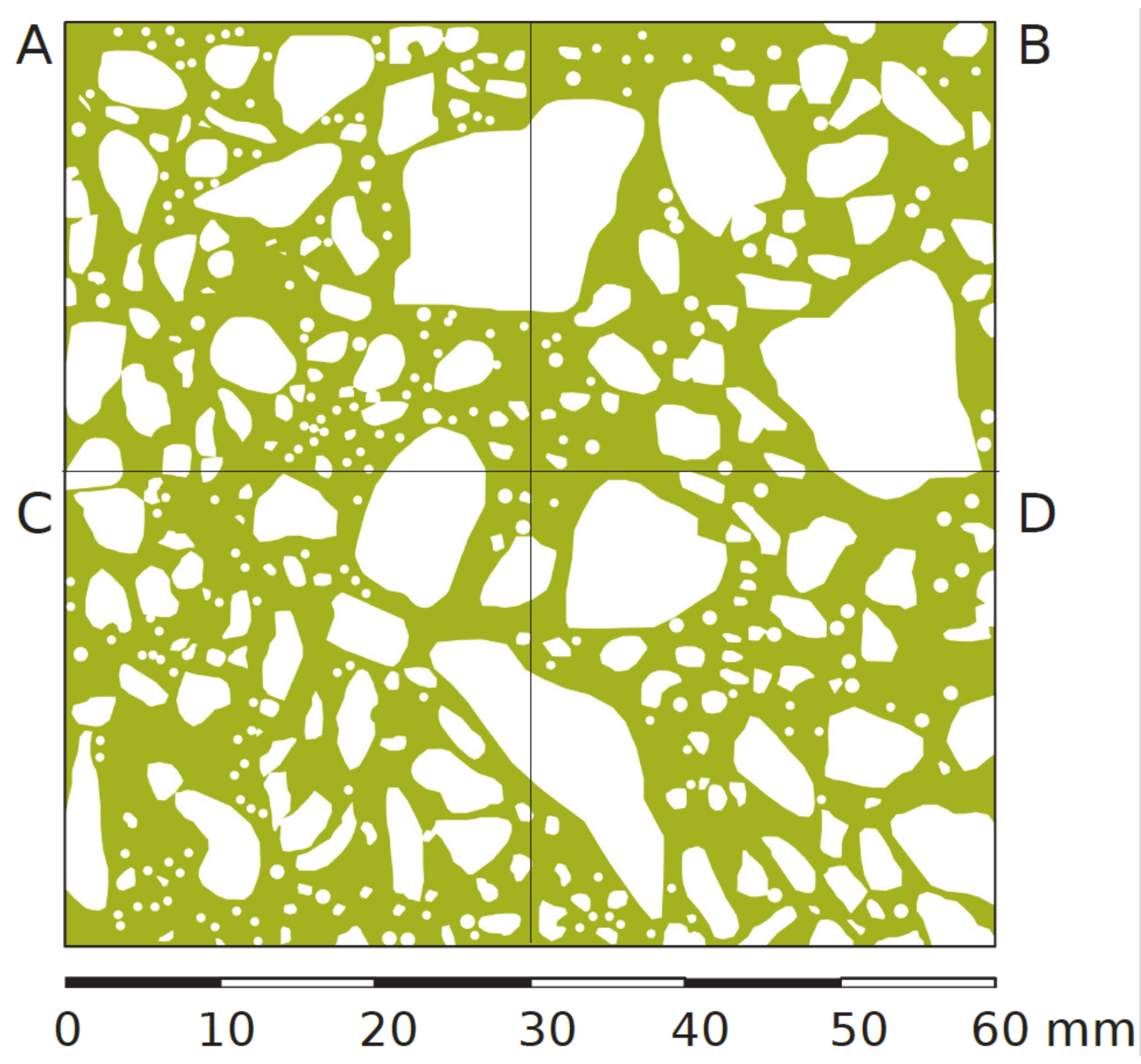
| Area | Unit | Concrete Area | Aggregates Area | Cement Matrix Area |
|---|---|---|---|---|
| A | [mm2] | 900 | 433 | 467 |
| [%] | 100 | 48.12 | 51.88 | |
| B | [mm2] | 900 | 445 | 455 |
| [%] | 100 | 49.48 | 50.52 | |
| C | [mm2] | 900 | 376 | 524 |
| [%] | 100 | 41.81 | 58.19 | |
| D | [mm2] | 900 | 416 | 484 |
| [%] | 100 | 46.22 | 53.78 | |
| A + B + C + D | [mm2] | 3600 | 1671 | 1929 |
| [%] | 100 | 46.41 | 53.59 |
| Model Name | Semivariogram | Equation No. |
|---|---|---|
| nugget | (3) | |
| linear with sill | (4) | |
| spherical | (5) | |
| exponential | (6) | |
| logarithmic | (7) |
| Parameter | Sample Number | ||||
|---|---|---|---|---|---|
| P0 | P20 | P21 | P22 | P23 | |
| Number of photos | 31 | 32 | 26 | 23 | 22 |
| Number of tie points | 191,205 | 185,801 | 184,875 | 126,506 | 146,182 |
| Total error of markers in mm | 0.26 | 0.30 | 0.32 | 0.27 | 0.26 |
| Total error of scale bars in mm | 0.16 | 0.16 | 0.14 | 0.16 | 0.15 |
| Original density of point model of concrete sample surface obtained from CRP after cutting to the size of 110 mm × 110 mm (points/mm2)/(points/inch2) | 225/145,161 | 282/181,935 | 269/173,548 | 263/169,677 | 250/161,290 |
| Sample Number | Semivariogram Type | Sill mm2 | Range mm | Method | Surface Type |
|---|---|---|---|---|---|
| P0 | Spherical | 0.0102 | 4.4744 | each pair from surface | not processed, mold touching |
| P0 | Spherical | 0.0980 | 4.513 | cop-x 1 | not processed, mold touching |
| P0 | Spherical | 0.0112 | 4.941 | cop-x45 2 | not processed, mold touching |
| P0 | Spherical | 0.0110 | 5.012 | cop-y 3 | not processed, mold touching |
| P20 | Spherical | 0.2536 | 10.675 | each pair from surface | sandblasting |
| P20 | Spherical | 0.2551 | 11.710 | cop-x 1 | sandblasting |
| P20 | Spherical | 0.2510 | 9.913 | cop-x45 2 | sandblasting |
| P20 | Spherical | 0.2548 | 12.017 | cop-y 3 | sandblasting |
| P21 | Expotential | 0.4832 | 8.6369 | each pair from surface | sandblasting |
| P21 | Expotential | 0.4838 | 8.6367 | cop-x 1 | sandblasting |
| P21 | Expotential | 0.4831 | 8.6353 | cop-x45 2 | sandblasting |
| P21 | Expotential | 0.4827 | 8.6367 | cop-y 3 | Sandblasting |
| P22 | Logarithmic | 0.0791 | 0.5139 | each pair from surface | Sandblasting |
| P23 | Exponential | 0.2366 | 10.4068 | each pair from surface | Sandblasting |
| Factor/ Parameter | B | A | C | Residual Sum-of- Squares | Number of Iterations to Convergence | Achieved Convergence Tolerance |
|---|---|---|---|---|---|---|
| Rvm | 0.752192 | 0.472575 | −0.008818 | 0.006090 | 8 | 5.463 × 10⁻⁸ |
| c | 0.58668 | 0.04188 | −0.216210 | 0.000370 | 10 | 2.483 × 10⁻⁶ |
| μ | 1.76614 | −0.01068 | 2.78001 | 0.0003032 | 6 | 1.009 × 10⁻⁶ |
© 2020 by the authors. Licensee MDPI, Basel, Switzerland. This article is an open access article distributed under the terms and conditions of the Creative Commons Attribution (CC BY) license (http://creativecommons.org/licenses/by/4.0/).
Share and Cite
Kozubal, J.; Wróblewski, R.; Muszyński, Z.; Wyjadłowski, M.; Stróżyk, J. Non-Deterministic Assessment of Surface Roughness as Bond Strength Parameters between Concrete Layers Cast at Different Ages. Materials 2020, 13, 2542. https://doi.org/10.3390/ma13112542
Kozubal J, Wróblewski R, Muszyński Z, Wyjadłowski M, Stróżyk J. Non-Deterministic Assessment of Surface Roughness as Bond Strength Parameters between Concrete Layers Cast at Different Ages. Materials. 2020; 13(11):2542. https://doi.org/10.3390/ma13112542
Chicago/Turabian StyleKozubal, Janusz, Roman Wróblewski, Zbigniew Muszyński, Marek Wyjadłowski, and Joanna Stróżyk. 2020. "Non-Deterministic Assessment of Surface Roughness as Bond Strength Parameters between Concrete Layers Cast at Different Ages" Materials 13, no. 11: 2542. https://doi.org/10.3390/ma13112542