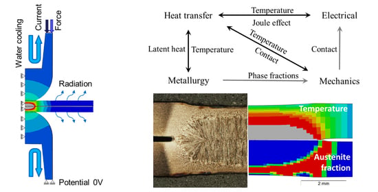
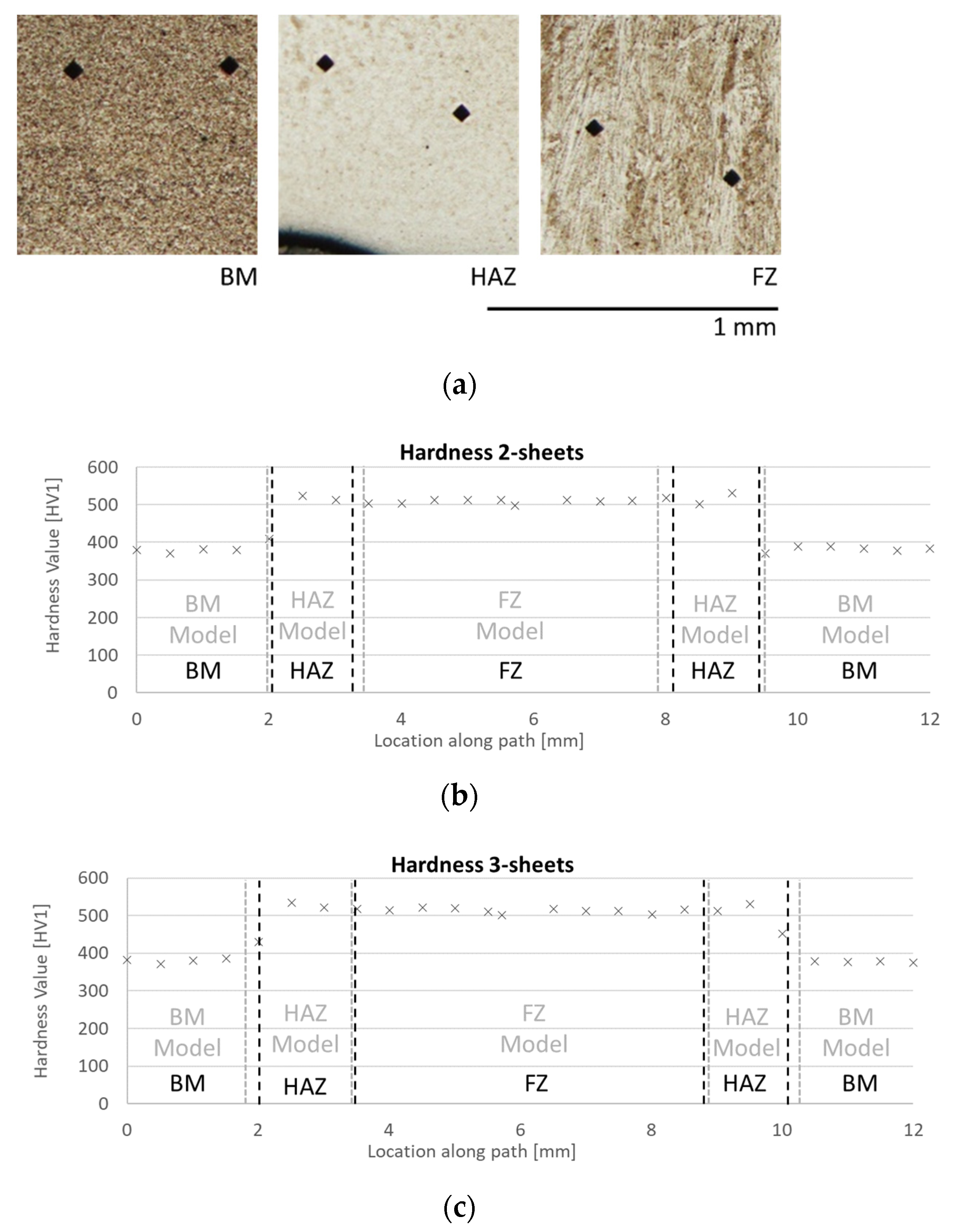
2.3.2. Material Model
The multi-physical material model couples the electrical-, thermal-, metallurgical- and mechanical problems. The electrical and thermal problem was solved with the built-in model capabilities of the commercial software package ABAQUS/Standard (version 2018, Dassault Systèmes, Vélizy-Villacoublay, France) whereas the metallurgical and mechanical material model equations were implemented by means of user-defined subroutines.
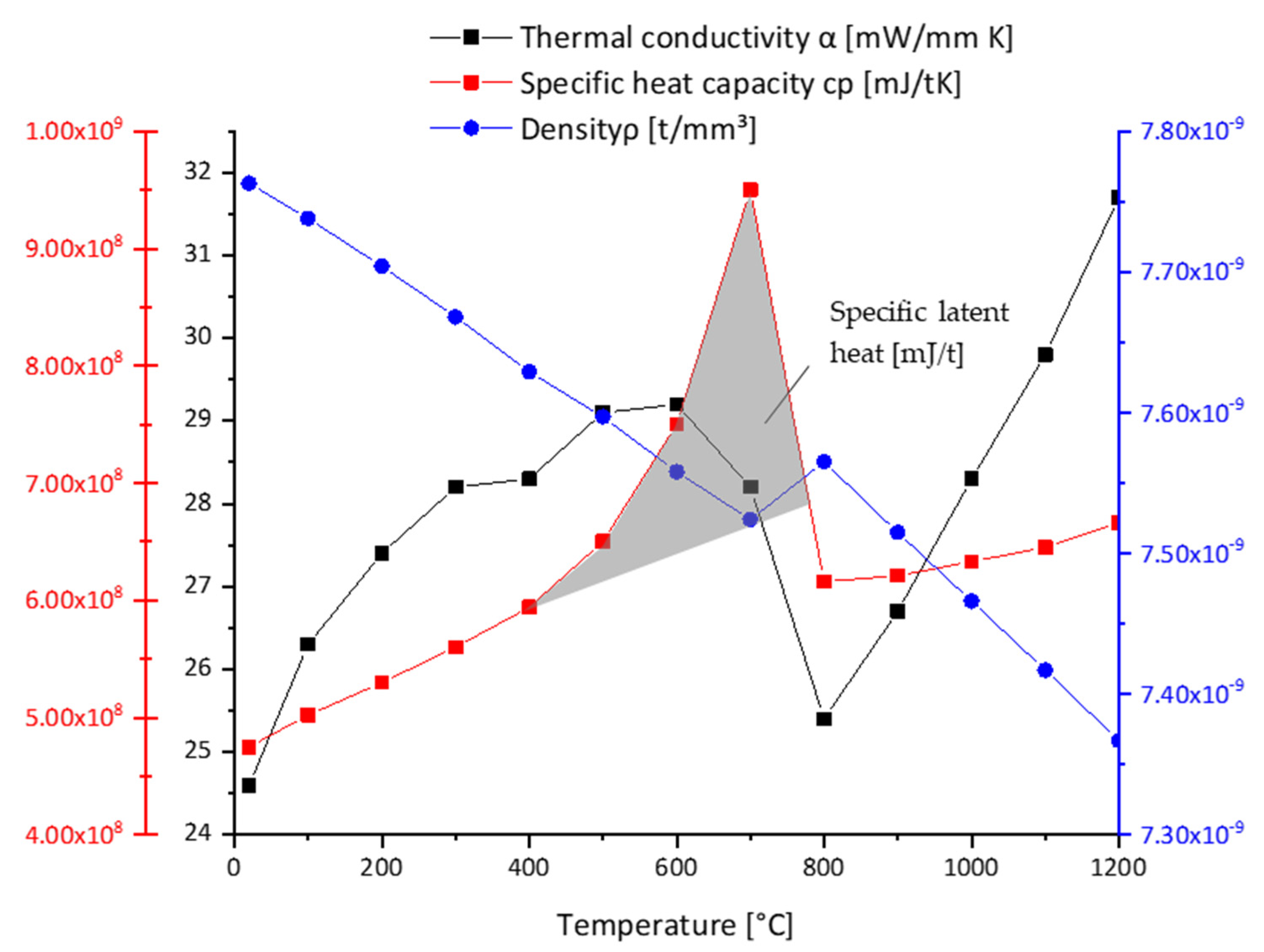
The measured temperature dependent thermal conductivity
λ, the specific heat capacity
cp, and the density
ρ are documented in
Figure 3 and a list of the implemented phase dependent values is provided in
Table 4.
For the sake of simplicity, the same material properties were applied for the base material and the martensitic phase and both are in this respect referred to as low temperature phase. The specific latent heat for the solid-to-solid phase transformation
LS was extracted from the calorimetric (DSC) measurement by calculating the area under the
cp–
T curve relative to the linearly extrapolated
cp–
T curve of the parent phase (see shaded area in
Figure 3). The so-calculated specific latent heat
LS was 9.1 × 10
10 mJ/t. The specific latent heat for the solid to liquid phase transformation
LL was taken based on the literature as 20.5 × 10
10 mJ/t [
39]. It was assumed that for all phase transformations the specific latent heat fraction scales linearly with the transformed phase fraction. The electrical conductivity
σe of the base material was calculated from the thermal conductivity
λ using the Wiedemann–Franz law [
27] given in Equation (1), where
T is the temperature and
L is the Lorentz number = 0.0244 mWmΩ/K
2. This data was then used as the initial guess in a first calculation run and subsequently adjusted by means of inverse parameter optimization. The temperature dependent electrical material conductivity
is summarized in
Table 5.
Since the difference between the electrical conductivity around the phase transformation temperature of the low temperature phase and austenite turned out to be similar a dependency on the phase state was omitted.
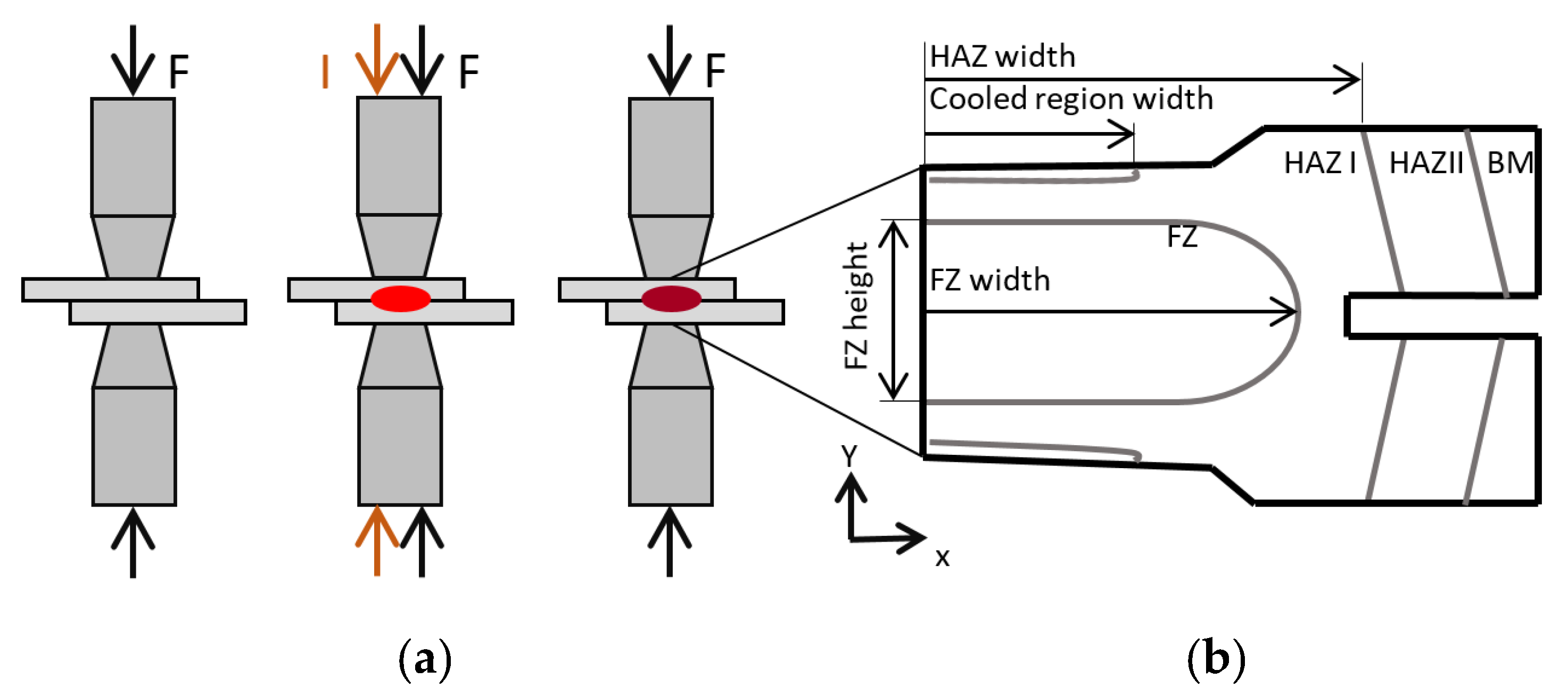
As described, joule heating causes the formation of a fusion zone between the sheets. The joule heating follows Equation (2), where
QW stands for the created thermal energy,
I for the current,
R for the electrical material resistance, and
t for time [
2]. For contact heating the electrical contact resistance
Rc, which is significantly higher than the electrical contact resistance
R, has to be considered in the calculation instead of
R.
A special focus of this work was set on the phase transformation model and its thermal and mechanical consequences based on strain rate and phase dependent material data, since this has not been treated in the literature in a similar rigorous form to that presented here. The phase transformation model was implemented by means of a set of user-defined Fortran 77 subroutines that combine four main aspects: (1) the phase transformation kinetics, (2) the latent heat generation, (3) the metallurgical strain caused by phase transformation, and (4) the formation of transformation induced plasticity. Furthermore, the thermal and mechanical material properties are modelled to be dependent on the phase fractions. The considered phases are the low temperature phase representing the base material and the martensitic state, the austenitic phase, and the liquid phase. The material properties of phase mixtures are calculated by means of a linear rule of mixture.
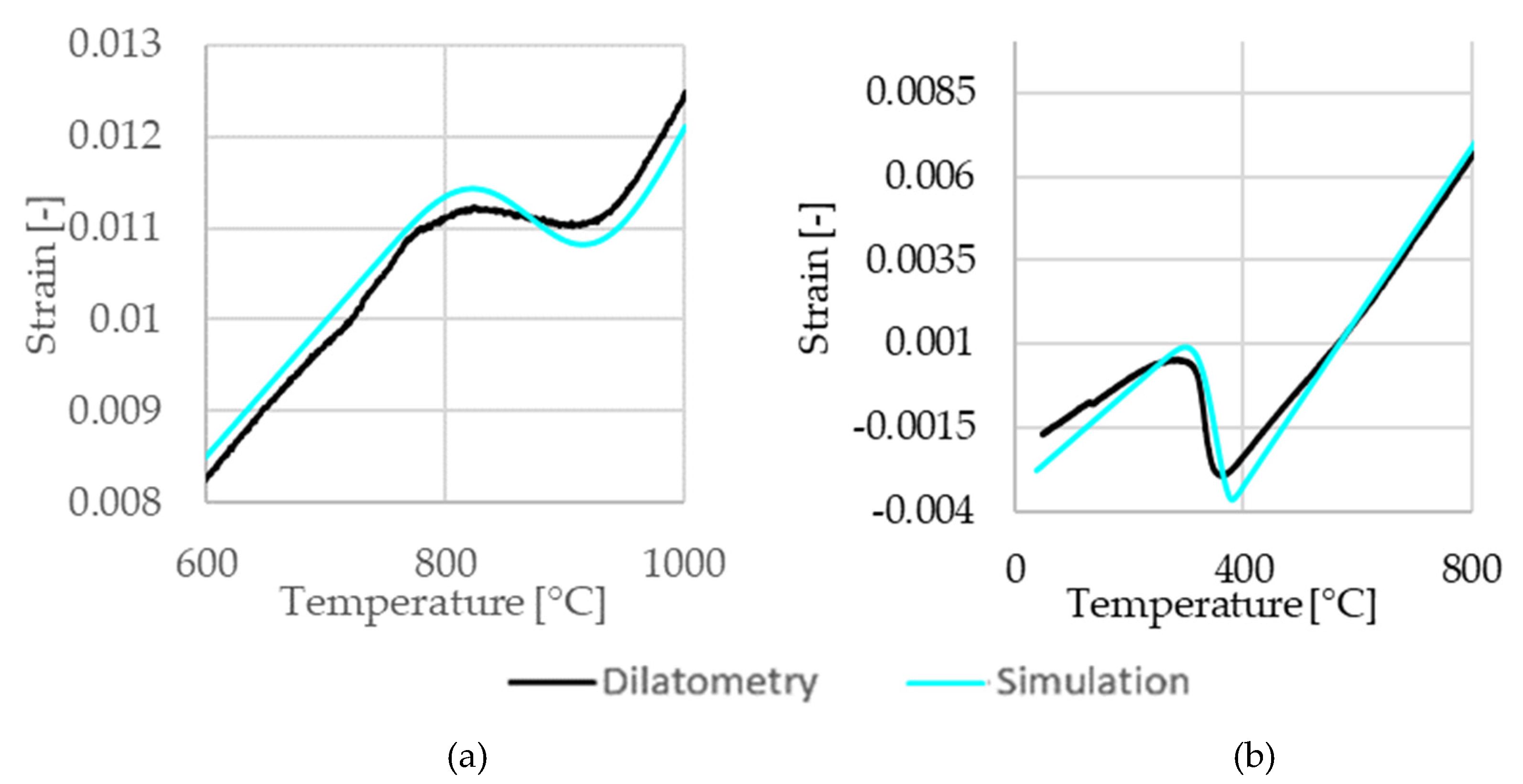
The phase transformation kinetics model for the solid-to-solid phase transformations is calibrated based on dilatometric tests with temperature rates of 3 °C/S, 100 °C/s and 400 °C/s.
Figure 4 shows the heating and cooling sequence of the experiment with a heating and cooling rate of 100 °C/s. Black lines indicate measured data and cyan lines indicate the respective simulation results. The phase changes of base material to austenite, austenite to liquid, and liquid to austenite are treated as diffusive phase transformations. The Scheil [
29] approach was used to convert the data obtained from isothermal TTT diagrams to continuous cooling conditions as prevalent in the actual welding process. Additionally, the Johnson–Mehl–Avrami–Kolomogorov (JMAK) [
40] kinetics given in Equation (3) was used, where
fx is the phase fraction of the newly created phase,
t is the time of isothermal holding,
k accounts for an overall rate constant, and
n is the Avrami coefficient.
The parameters applied for the JMAK model for solid-to-solid phase transformation from base material to austenite were k = 6.65 × 10³ and n = 2 at a rate of 1000 °C/s, for austenite–liquid transformation k = 5 × 10³ and n = 2 and for liquid–solid transformation k = 6.65 and n = 2. The kinetics parameters of the latter two phase transformations were determined based on ThermoCalc 2017 (Thermo-Calc Software AB, Solna, Sweden) calculations.
The Koistinen–Marburger kinetics [
41], shown in Equation (4), was chosen to describe the solid state transformation from austenite to martensite.
fM is the volume fraction of martensite,
MS is the martensite start temperature,
T describes the current temperature,
fγ is the volume fraction of austenite, and
a is the Koistinen–Marburger parameter [
41]. A Koistinen–Marburger parameter of 0.011 led to a good match between the experimental results and the model. Due to rapid cooling no other phases besides martensite are formed.
The mechanical problem is formulated in the small strain regime. Hence, the total strain tensor
can be decomposed into different strain contributions as seen in Equation (5). In the present case these strain contributions are elastic strain
, thermal strain
, metallurgical strain
, plastic strain
(due to classical plasticity), and transformation induced plasticity strain
.
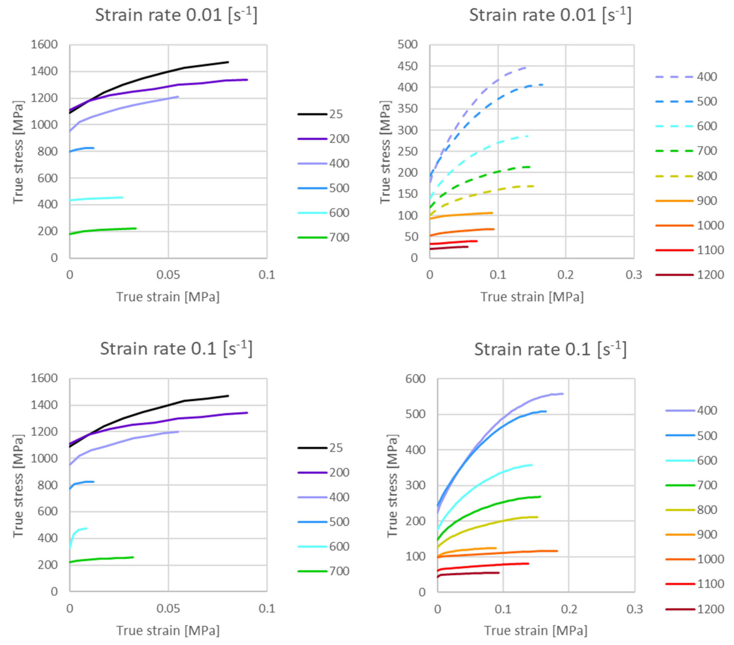
The elastic material properties were defined for both the low temperature phase and the austenitic phase in a temperature dependent form. The Young’s moduli and the Poissons’s ratios were taken from [
42] and [
25], respectively. For the liquid phase a quasi-solid elastic body with a Poisson’s ratio of 0.48 and a Young’s modulus of 1 GPa was assumed. The elastic properties are summarized in
Table 6.
The mean coefficient of thermal expansion
αCTE was measured to be 1.478 × 10
5 K
−1 between 20 °C and 500 °C for the base material and 2.52 × 10
5 K
−1 for temperatures ranging from 900 °C to 1200 °C for austenite. For the liquid steel melt which appears above about 1500 °C the thermal expansion coefficient was taken from the literature as 4.0 × 10
5 K
−1 [
43]. The metallurgical strain between the low temperature phase and the austenitic phase accounts for the transformation dilatational strain, however, corrected for the thermal expansion in the transformation window [
44]. The plastic yield stress and the isotropic hardening evolution were defined by means of tabular data depending on temperature, strain rate and phase type. The plastic flow curves were measured for the low temperature phase (base material) and austenite for temperatures up to 700 °C and 1200 °C, respectively, and for four strain rates between 0.01 s
−1 to 10 s
−1. The set of implemented flow curves is shown in
Figure 5. The dashed lines indicate extrapolated data for the metastable austenite following the procedure proposed in [
25].
The rate of the accumulated strain is abbreviated as strain rate. The transformation induced plasticity strain tensor
is in the current case only relevant for the austenite to martensite transformation. It was calculated according to Equation (6), with
as the stress deviator,
as the saturation function with a maximum of 1,
describes the time derivative of the volume fraction of the product phase and
denotes the time increment [
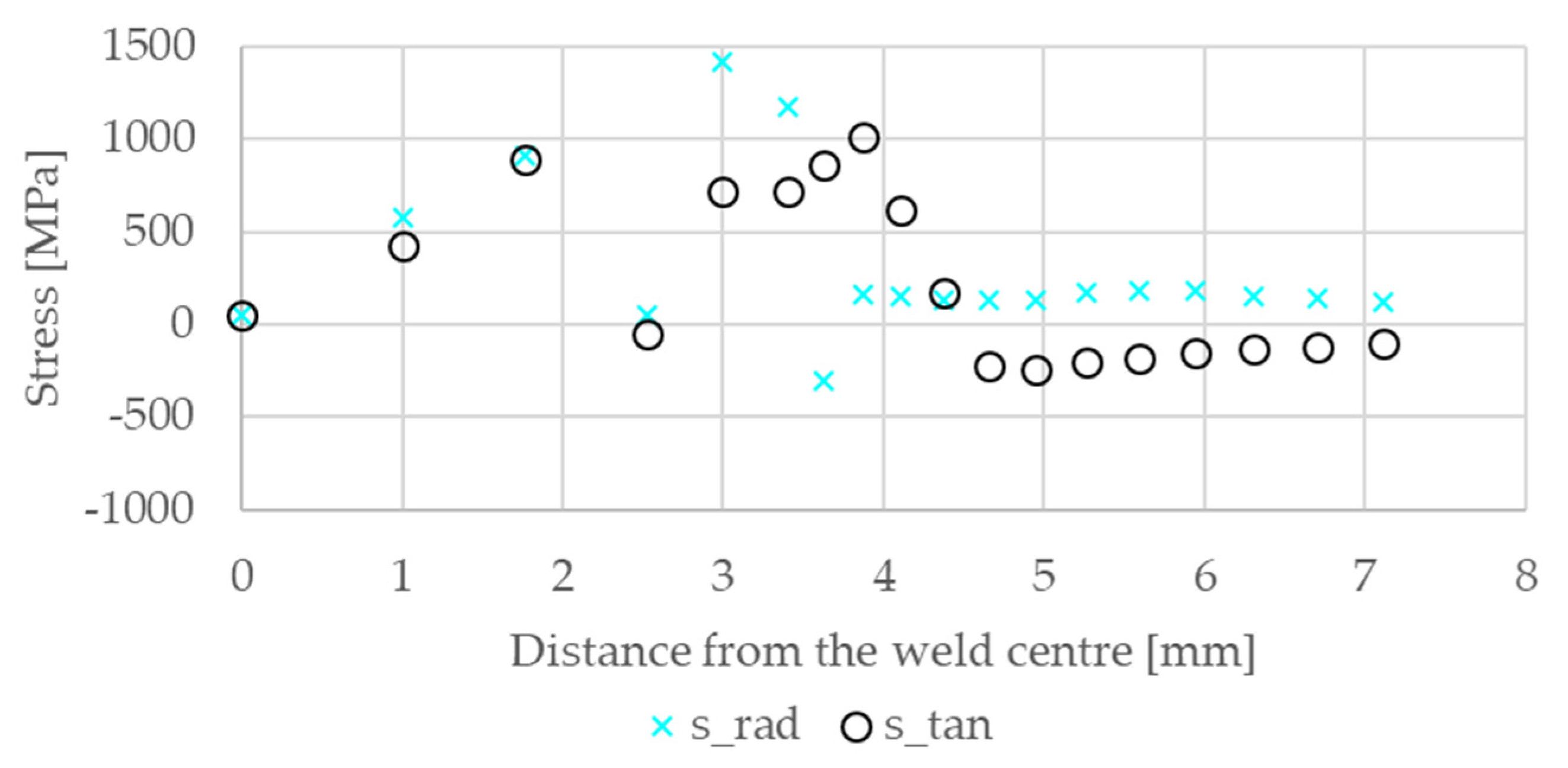
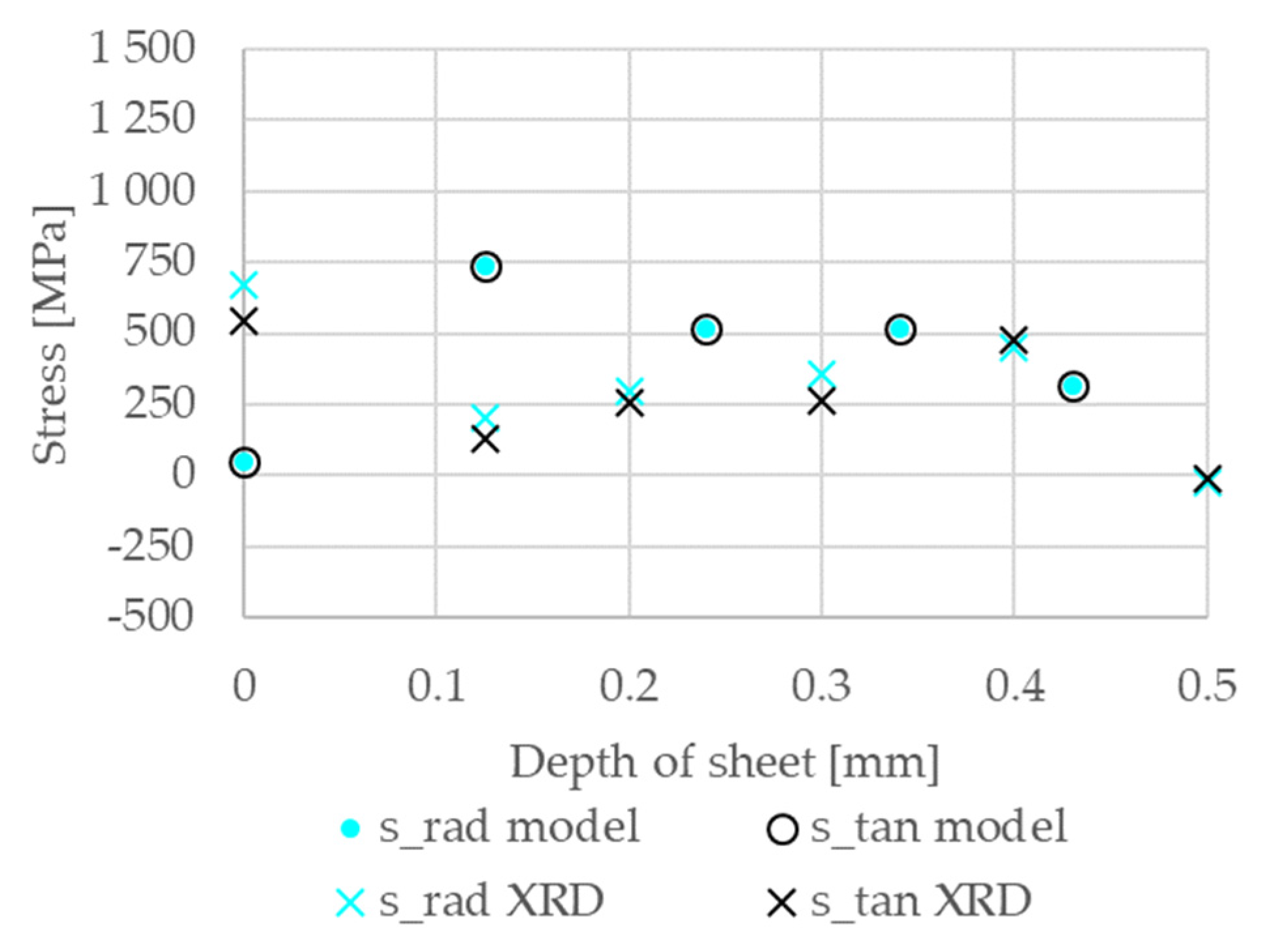
44]. The Greenwood-Johnson parameter was determined experimentally from dilatometry under load to be
× 10
5 MPa
−1.
The material data for the copper–chrome–zircon electrodes were taken from the literature [
45,
46].
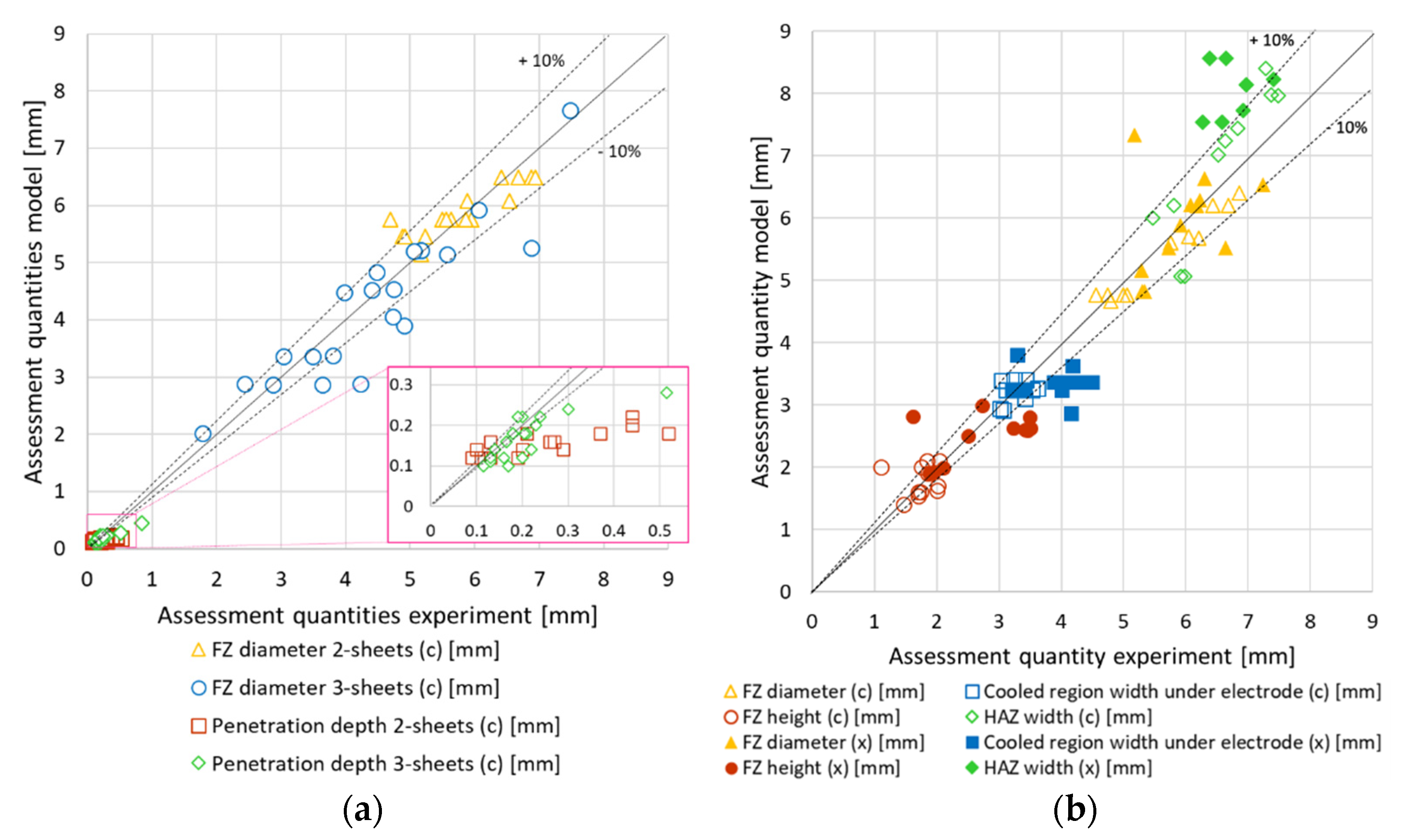
The full set of mainly experimentally determined model parameters and the consideration of the evolution of the metallurgical fields and their related quantities governed by phase transformation kinetics models allow a realistic model description of the RSW process and the evolution of the local quantity fields.


