
Comparison of CAD and Voxel-Based Modelling Methodologies for the Mechanical Simulation of Extrusion-Based 3D Printed Scaffolds

 ,
,  , and
, and
Abstract
:1. Introduction
2. Materials and Methods
2.1. Materials
2.2. Geometries and Manufacturing Parameters
2.3. Modelling Methods
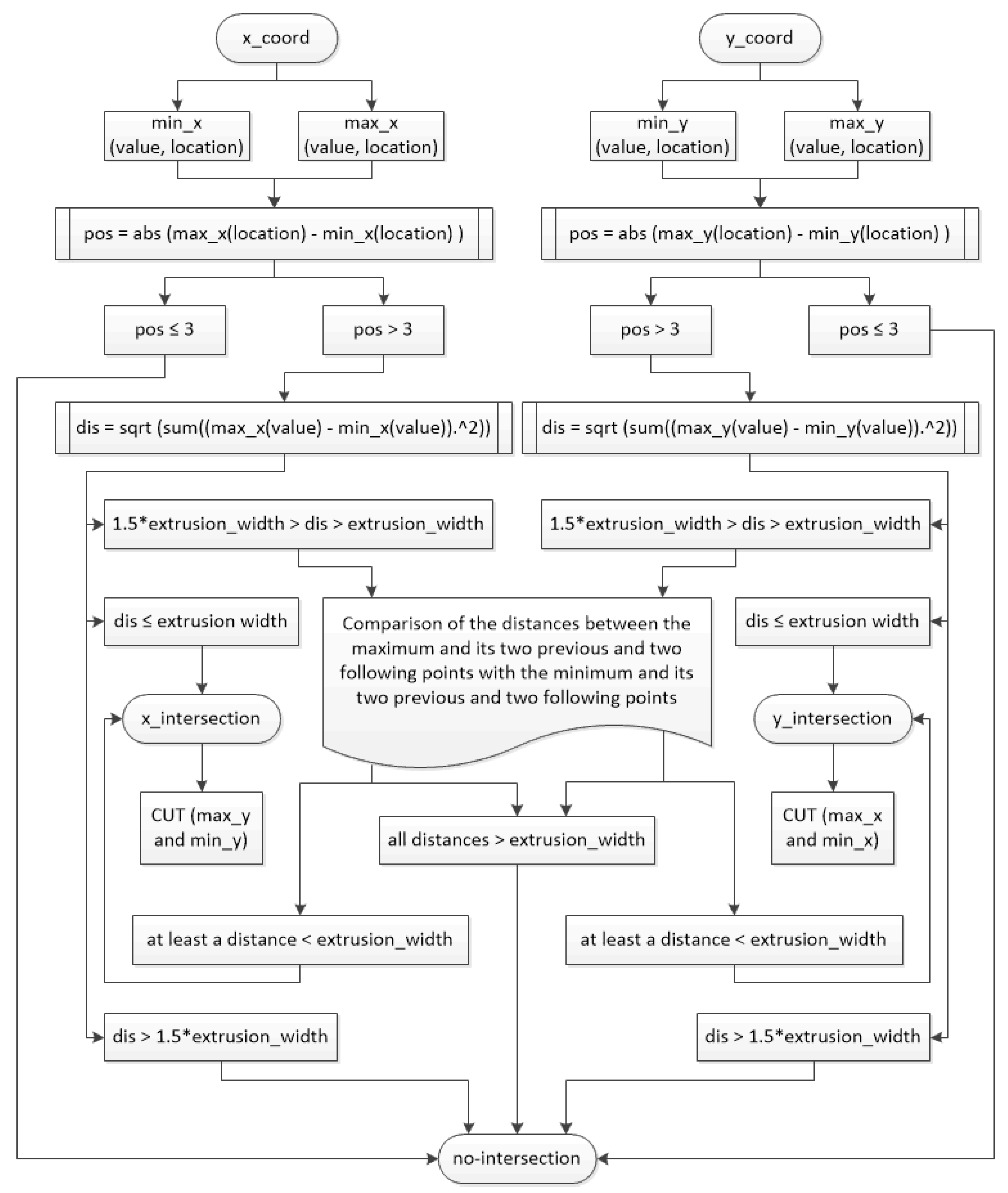
2.3.1. G-Code Conditioning
2.3.2. Voxel-Based Modelling (VOLCO)
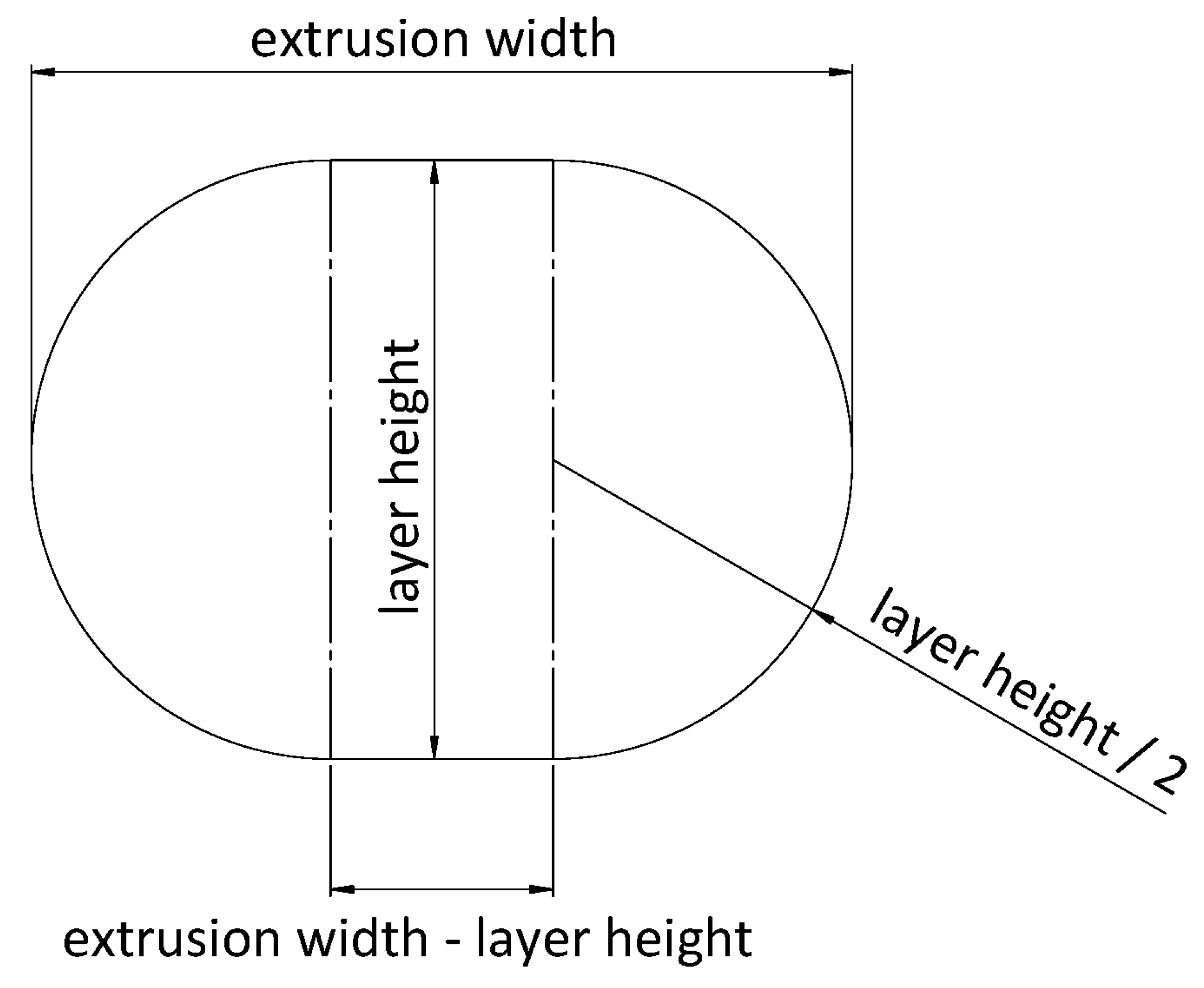
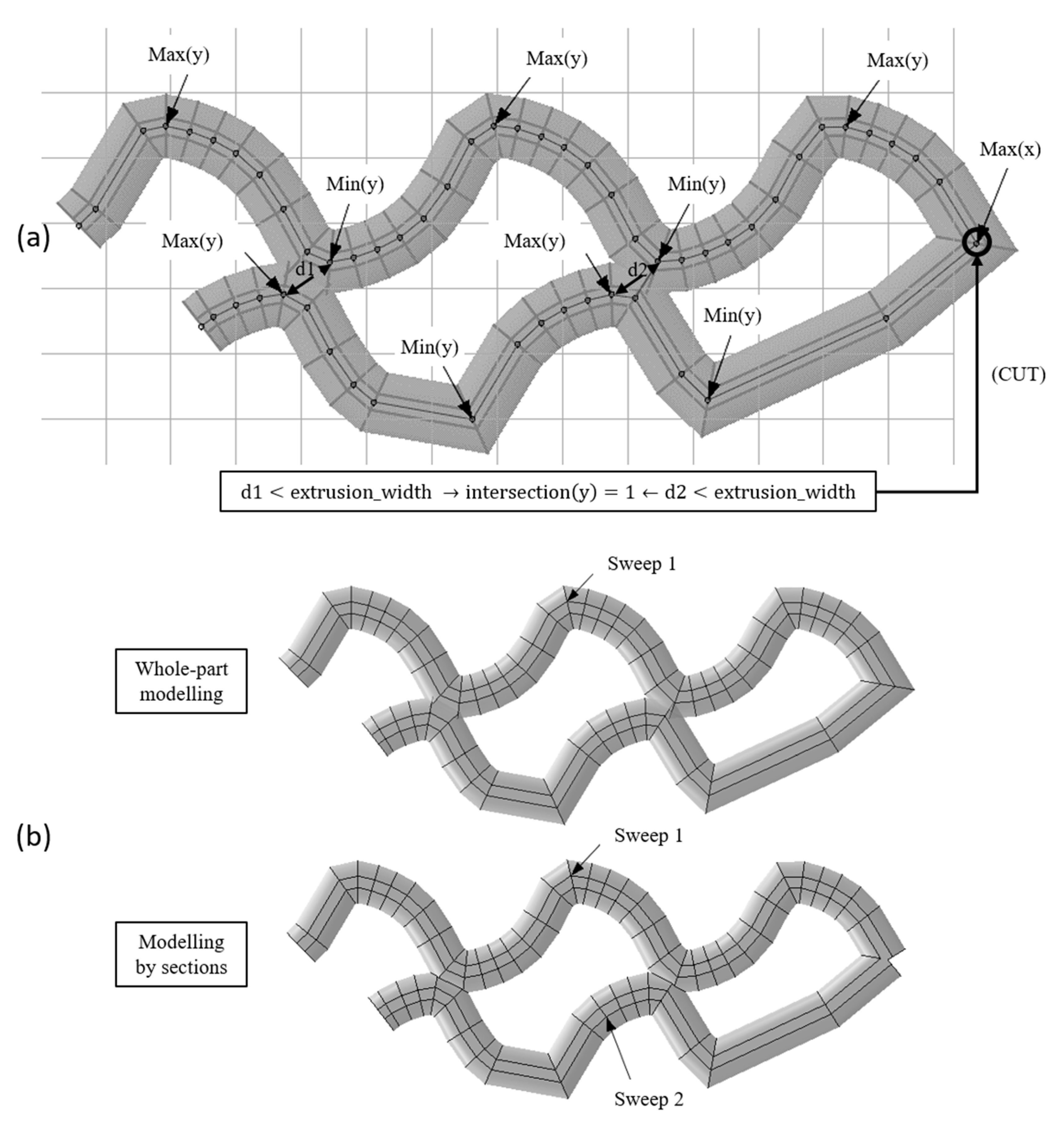
2.3.3. Geometry-Based Modelling
- 1.
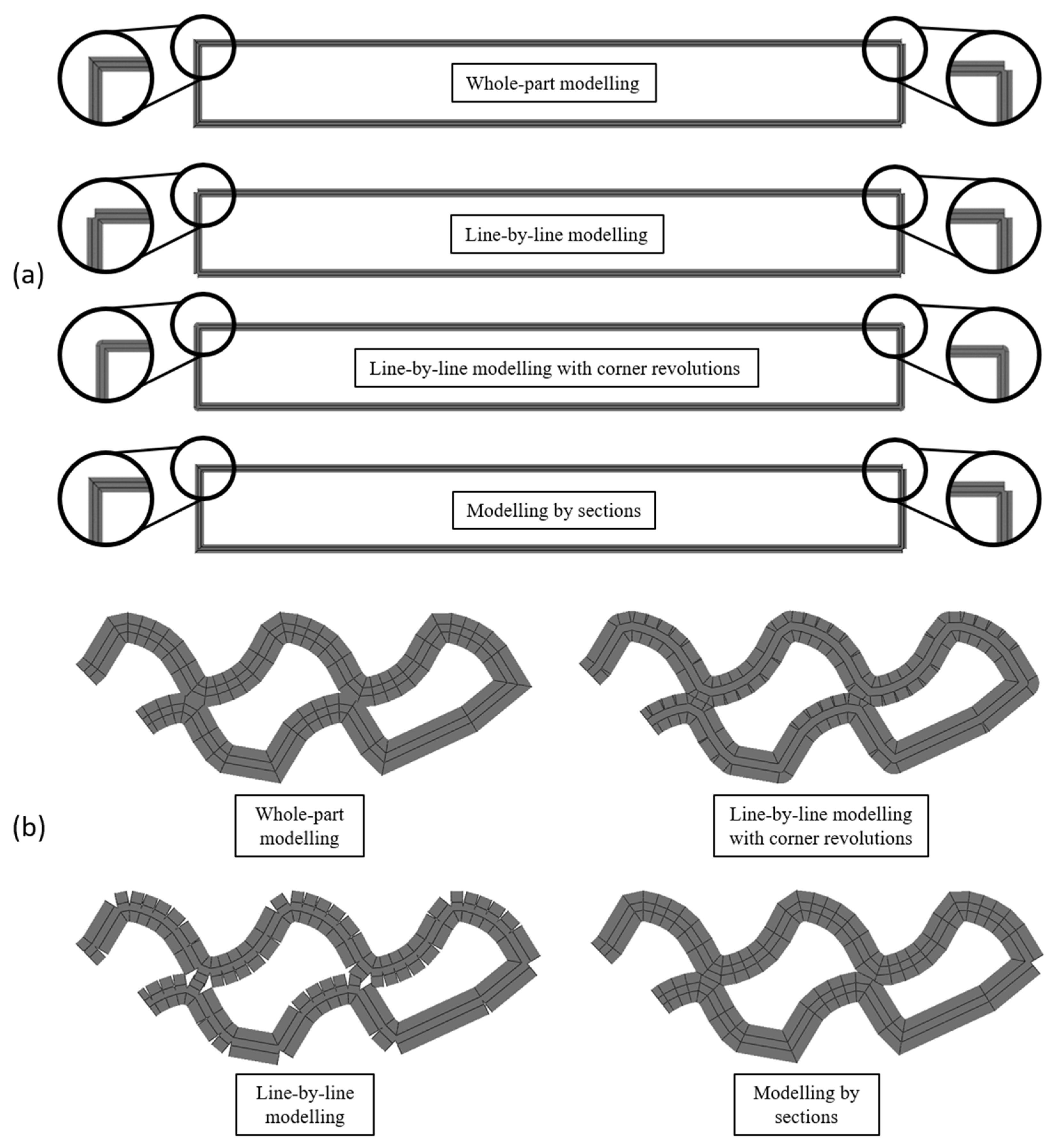
- Whole-Part Modelling
- 2.
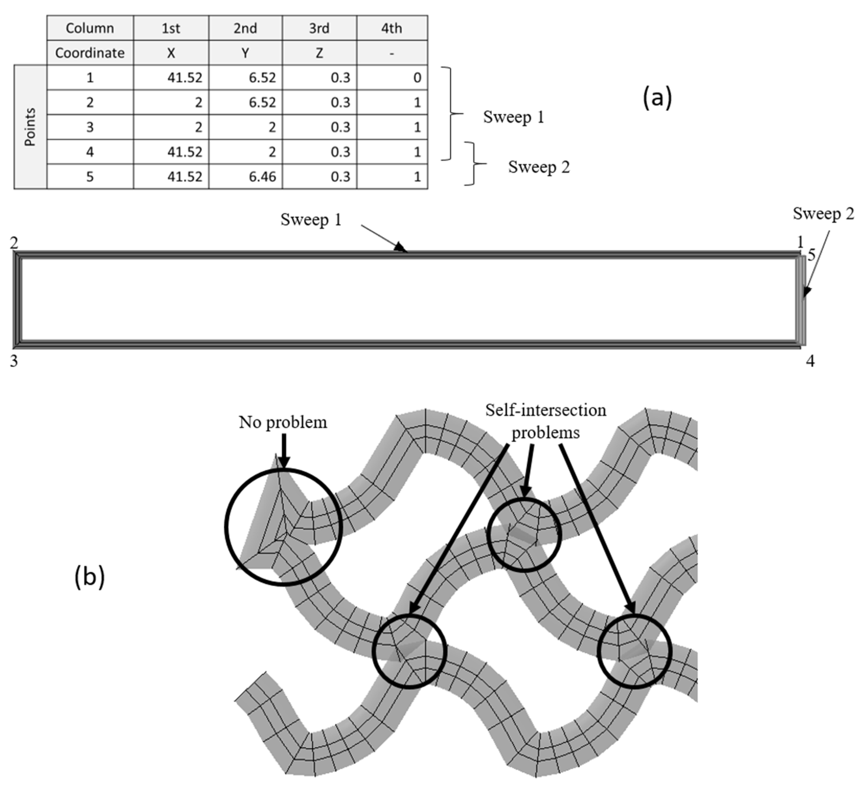
- Line-by-Line Modelling
- 3.
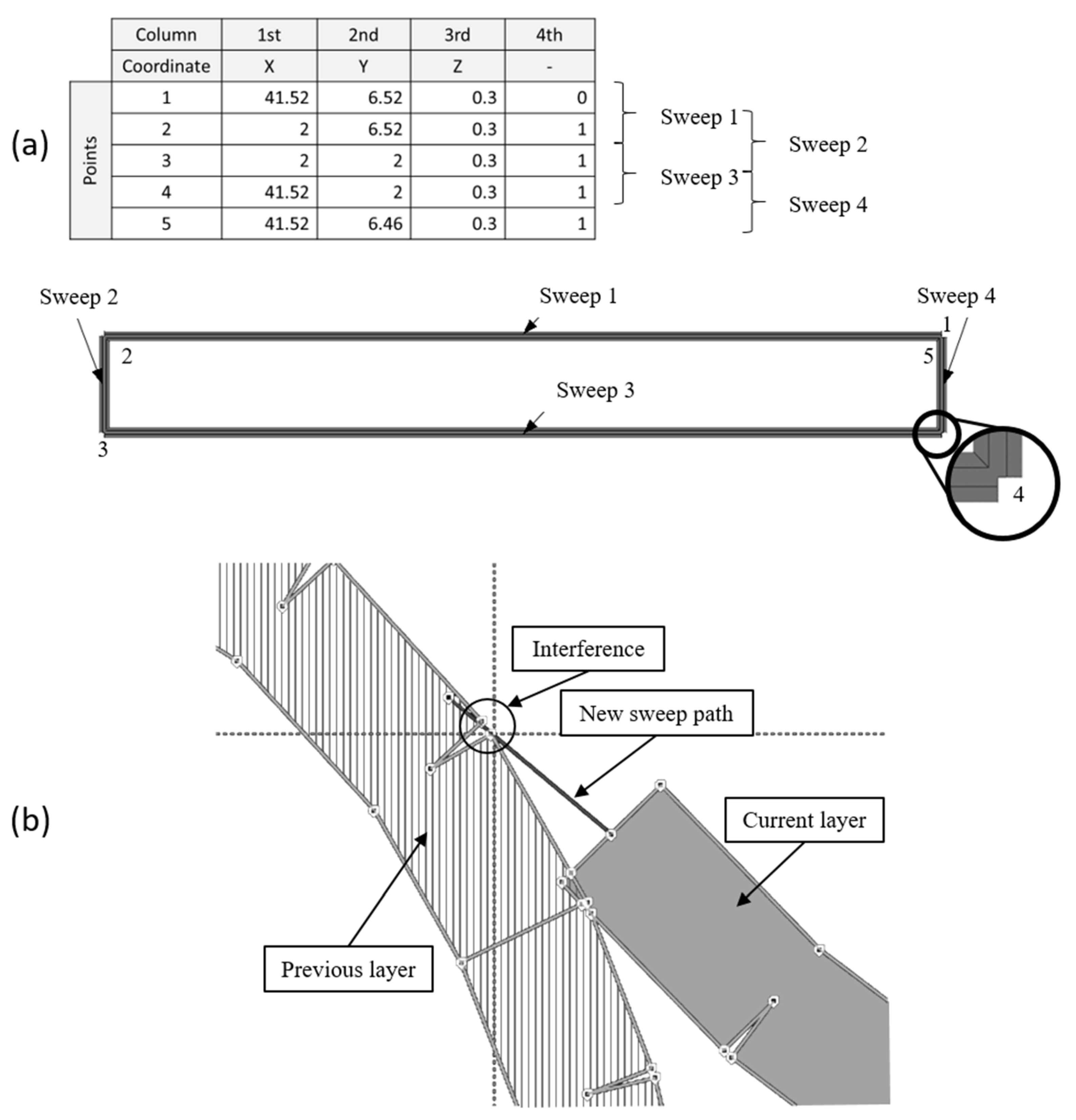
- Line-by-Line Modelling with Corner Revolutions
- 4.
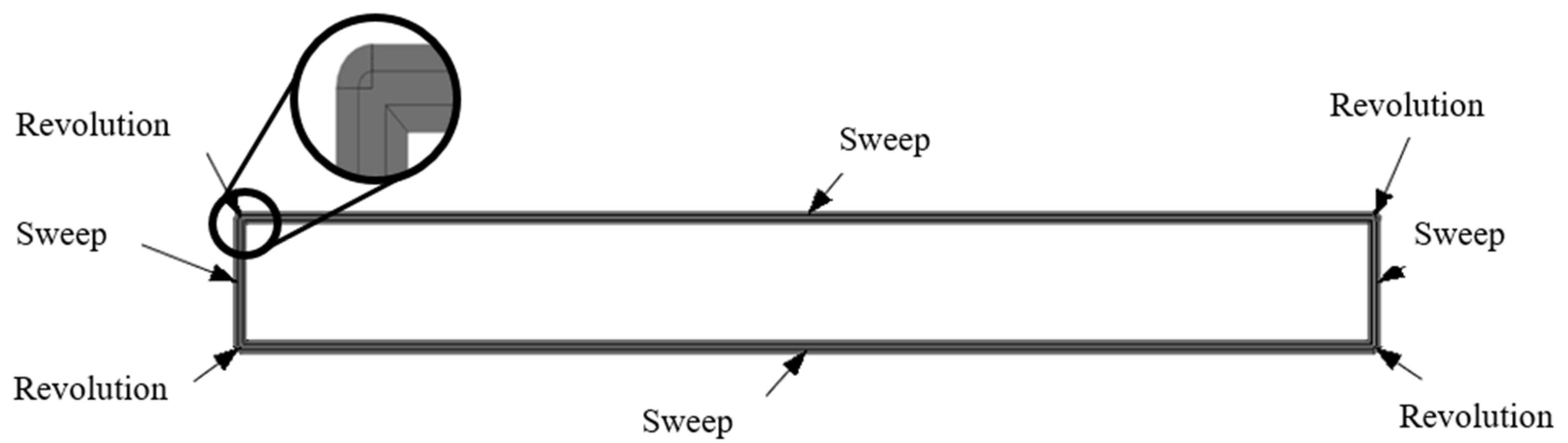
- Modelling by Sections
- 5.
- Comparison of Modelling Strategies
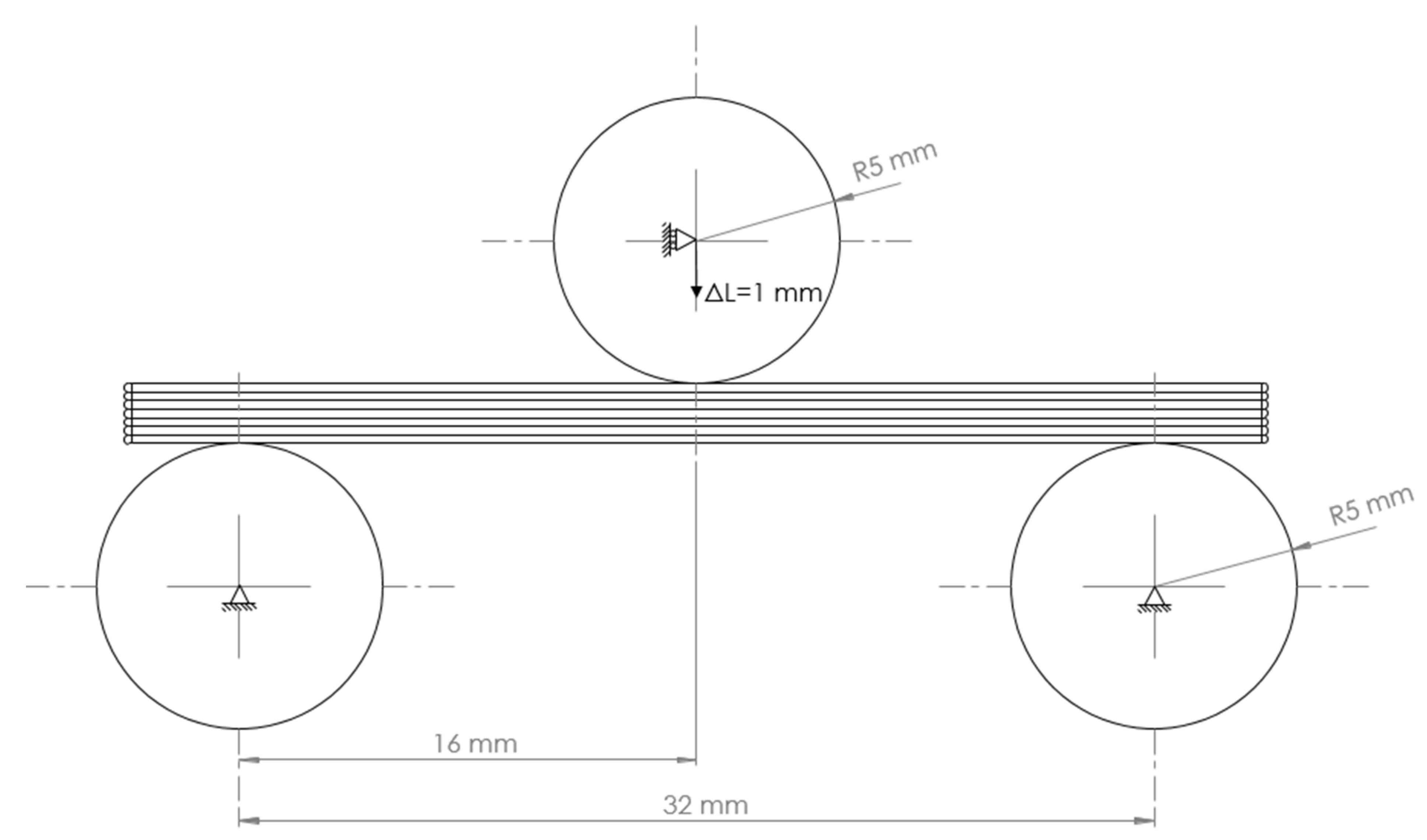
2.3.4. Compression Simulation by Finite Element Analysis
2.4. Scaffold Manufacturing and Compression Tests
2.5. Morphological Characterisation
3. Results and Discussion
3.1. Modelling Efficiency
3.1.1. Scaffold Modelling Efficiency
3.1.2. Modelling Limitations
3.2. Dimensional Accuracy
3.2.1. Volume
3.2.2. Dimensions and Shape
3.3. Equivalent Elastic Modulus
4. Conclusions
Supplementary Materials
Author Contributions
Funding
Institutional Review Board Statement
Informed Consent Statement
Data Availability Statement
Conflicts of Interest
References
- Perez, R.A.; Mestres, G. Role of pore size and morphology in musculo-skeletal tissue regeneration. Mater. Sci. Eng. C 2016, 61, 922–939. [Google Scholar] [CrossRef]
- Chuenjitkuntaworn, B.; Inrung, W.; Damrongsri, D.; Mekaapiruk, K.; Supaphol, P.; Pavasant, P. Polycaprolactone/Hydroxyapatite composite scaffolds: Preparation, characterization, and in vitro and in vivo biological responses of human primary bone cells. J. Biomed. Mater. Res. Part A 2010, 10. [Google Scholar] [CrossRef]
- Gómez-Lizárraga, K.K.; Flores-Morales, C.; Del Prado-Audelo, M.L.; Álvarez-Pérez, M.A. Polycaprolactone-and polycaprolactone/ceramic-based 3D-bioplotted porous scaffolds for bone regeneration: A comparative study. Mater. Sci. Eng. C 2017, 79, 326–335. [Google Scholar] [CrossRef] [PubMed]
- Chen, S.; Guo, Y.; Liu, R.; Wu, S.; Fang, J.; Huang, B.; Li, Z.; Chen, Z.; Chen, Z. Tuning surface properties of bone biomaterials to manipulate osteoblastic cell adhesion and the signaling pathways for the enhancement of early osseointegration. Colloids Surfaces B Biointerfaces 2018, 164, 58–69. [Google Scholar] [CrossRef] [PubMed]
- Karageorgiou, V.; Kaplan, D. Porosity of 3D biomaterial scaffolds and osteogenesis. Biomaterials 2005, 26, 5474–5491. [Google Scholar] [CrossRef] [PubMed]
- Agrawal, C.M.; Mckinney, J.S.; Lanctot, D.; Athanasiou, K.A. Effects of fluid flow on the in vitro degradation kinetics of biodegradable scaffolds for tissue engineering. Biomaterials 2000, 21, 2443–2452. [Google Scholar] [CrossRef]
- Bosworth, L.A.; Downes, S. Physicochemical characterisation of degrading polycaprolactone scaffolds. Polym. Degrad. Stab. 2010, 95, 2269–2276. [Google Scholar] [CrossRef]
- Hendrikson, W.J.; van Blitterswijk, C.A.; Rouwkema, J.; Moroni, L. The Use of Finite Element Analyses to Design and Fabricate Three-Dimensional Scaffolds for Skeletal Tissue engineering. Front. Bioeng. Biotechnol. 2017, 5, 1–13. [Google Scholar] [CrossRef] [PubMed] [Green Version]
- Velasco, M.A.; Narváez-Tovar, C.A.; Garzón-Alvarado, D.A. Design, Materials, and Mechanobiology of Biodegradable Scaffolds for Bone Tissue Engineering. Biomed Res. Int. 2015, 2015. [Google Scholar] [CrossRef] [PubMed]
- Naghieh, S.; Karamooz Ravari, M.R.; Badrossamay, M.; Foroozmehr, E.; Kadkhodaei, M. Numerical investigation of the mechanical properties of the additive manufactured bone scaffolds fabricated by FDM: The effect of layer penetration and post-heating. J. Mech. Behav. Biomed. Mater. 2016, 59, 241–250. [Google Scholar] [CrossRef] [Green Version]
- Seol, Y.-J.; Kang, H.-W.; Lee, S.J.; Atala, A.; Yoo, J.J. Bioprinting technology and its applications. Eur. J. Cardio-Thoracic Surg. 2014, 46, 342–348. [Google Scholar] [CrossRef] [Green Version]
- Ribeiro, J.F.M.; Oliveira, S.M.; Alves, J.L.; Pedro, A.J.; Reis, R.L.; Fernandes, E.M.; Mano, J.F. Structural monitoring and modeling of the mechanical deformation of three-dimensional printed poly (ε-caprolactone) scaffolds. Biofabrication 2017, 9, 025015. [Google Scholar] [CrossRef] [Green Version]
- Qu, H. Additive manufacturing for bone tissue engineering scaffolds. Mater. Today Commun. 2020, 24, 1–16. [Google Scholar] [CrossRef]
- Saygili, E.; Dogan-Gurbuz, A.A.; Yesil-Celiktas, O.; Draz, M.S. 3D bioprinting: A powerful tool to leverage tissue engineering and microbial systems. Bioprinting 2020, 18, e00071. [Google Scholar] [CrossRef]
- Singh, D.; Babbar, A.; Jain, V.; Gupta, D.; Saxena, S.; Dwibedi, V. Synthesis, characterization, and bioactivity investigation of biomimetic biodegradable PLA scaffold fabricated by fused filament fabrication process. J. Brazilian Soc. Mech. Sci. Eng. 2019, 41, 1–13. [Google Scholar] [CrossRef]
- Temple, J.P.; Hutton, D.L.; Hung, B.P.; Huri, P.Y.; Cook, C.A.; Kondragunta, R.; Jia, X.; Grayson, W.L. Engineering anatomically shaped vascularized bone grafts with hASCs and 3D-printed PCL scaffolds. J. Biomed. Mater. Res. Part A 2014, 102, 4317–4325. [Google Scholar] [CrossRef] [PubMed]
- Roopavath, U.K.; Malferrari, S.; Van Haver, A.; Verstreken, F.; Rath, S.N.; Kalaskar, D.M. Optimization of extrusion based ceramic 3D printing process for complex bony designs. Mater. Des. 2019, 162, 263–270. [Google Scholar] [CrossRef]
- Sahai, N.; Saxena, K.K.; Gogoi, M. Modelling and simulation for fabrication of 3D printed polymeric porous tissue scaffolds. Adv. Mater. Process. Technol. 2020, 1–10. [Google Scholar] [CrossRef]
- Souness, A.; Zamboni, F.; Walker, G.M.; Collins, M.N. Influence of scaffold design on 3D printed cell constructs. J. Biomed. Mater. Res. Part B 2018, 106B, 533–545. [Google Scholar] [CrossRef]
- Soufivand, A.A.; Abolfathi, N.; Hashemi, S.A.; Lee, S.J. Prediction of mechanical behavior of 3D bioprinted tissue-engineered scaffolds using finite element method (FEM) analysis. Addit. Manuf. 2020, 33, 2214–8604. [Google Scholar] [CrossRef]
- Schipani, R.; Nolan, D.R.; Lally, C.; Kelly, D.J. Integrating finite element modelling and 3D printing to engineer biomimetic polymeric scaffolds for tissue engineering. Connect. Tissue Res. 2020, 61, 174–189. [Google Scholar] [CrossRef]
- Miranda, P.; Pajares, A.; Guiberteau, F. Finite element modeling as a tool for predicting the fracture behavior of robocast scaffolds. Acta Biomater. 2008, 4, 1715–1724. [Google Scholar] [CrossRef]
- Entezari, A.; Fang, J.; Sue, A.; Zhang, Z.; Swain, M.V.; Li, Q. Yielding behaviors of polymeric scaffolds with implications to tissue engineering. Mater. Lett. 2016, 184, 108–111. [Google Scholar] [CrossRef]
- Melancon, D.; Bagheri, Z.S.; Johnston, R.B.; Liu, L.; Tanzer, M.; Pasini, D. Mechanical characterization of structurally porous biomaterials built via additive manufacturing: Experiments, predictive models, and design maps for load-bearing bone replacement implants. Acta Biomater. 2017, 63, 350–368. [Google Scholar] [CrossRef]
- Kadkhodapour, J.; Montazerian, H.; Darabi, A.C.; Anaraki, A.P.; Ahmadi, S.M.; Zadpoor, A.A.; Schmauder, S. Failure mechanisms of additively manufactured porous biomaterials: Effects of porosity and type of unit cell. J. Machanical Behav. Biomed. Mater. 2015, 50, 180–191. [Google Scholar] [CrossRef] [PubMed]
- Campoli, G.; Borleffs, M.S.; Amin Yavari, S.; Wauthle, R.; Weinans, H.; Zadpoor, A.A. Mechanical properties of open-cell metallic biomaterials manufactured using additive manufacturing. Mater. Des. 2013, 49, 957–965. [Google Scholar] [CrossRef]
- Ravari, M.R.K.; Kadkhodaei, M.; Badrossamay, M.; Rezaei, R. Numerical investigation on mechanical properties of cellular lattice structures fabricated by fused deposition modeling. Int. J. Mech. Sci. 2014, 88, 154–161. [Google Scholar] [CrossRef]
- Gleadall, A.; Ashcroft, I.; Segal, J. VOLCO: A predictive model for 3D printed microarchitecture. Addit. Manuf. 2018, 21, 605–618. [Google Scholar] [CrossRef]
- Sanz-Herrera, J.A.; García-Aznar, J.M.; Doblaré, M. On scaffold designing for bone regeneration: A computational multiscale approach. Acta 2009, 5, 219–229. [Google Scholar] [CrossRef]
- Rupal, B.S.; Mostafa, K.G.; Wang, Y.; Qureshi, A.J. A Reverse CAD Approach for Estimating Geometric and Mechanical A Reverse CAD Approach for Estimating Geometric and Mechanical Behavior of FDM Conference Printed Parts Behavior of FDM Printed Parts Costing models for capacity optimization Trade-off between. Procedia Manuf. 2019, 34, 535–544. [Google Scholar] [CrossRef]
- Sukindar, N.A.; Dahan, A.A.A.; Halim, N.F.H.A.; Kamaruddin, S.; Sulaiman, M.H.; Ariffin, M.K.A.M. The Effect of Printing Parameters on Scaffold Structure Using Low-cost 3D Printer. Test Eng. Manag. 2020, 82, 8255–8263. [Google Scholar]
- Hollister, S.J. Porous scaffold design for tissue engineering. Nat. Mater. 2005, 4, 518–524. [Google Scholar] [CrossRef]
- Giannitelli, S.M.; Accoto, D.; Trombetta, M.; Rainer, A. Current trends in the design of scaffolds for computer-aided tissue engineering. Acta Biomater. 2014, 10, 580–594. [Google Scholar] [CrossRef] [PubMed]
- Gómez, S.; Vlad, M.D.; López, J.; Fernández, E. Design and properties of 3D scaffolds for bone tissue engineering. Acta Biomater. 2016, 42, 341–350. [Google Scholar] [CrossRef] [PubMed]
- Wang, G.; Shen, L.; Zhao, J.; Liang, H.; Xie, D.; Tian, Z.; Wang, C. Design and Compressive Behavior of Controllable Irregular Porous Scaffolds: Based on Voronoi-Tessellation and for Additive Manufacturing. ACS Biomater. Sci. Eng. 2018, 4, 719–727. [Google Scholar] [CrossRef] [PubMed]
- Bellehumeur, C.; Li, L.; Sun, Q.; Gu, P. Modeling of bond formation between polymer filaments in the fused deposition modeling process. J. Manuf. Process. 2004, 6, 170–178. [Google Scholar] [CrossRef]
- Park, S.; Rosen, D.W. Quantifying effects of material extrusion additive manufacturing process on mechanical properties of lattice structures using as-fabricated voxel modeling. Addit. Manuf. 2016, 12, 265–273. [Google Scholar] [CrossRef] [Green Version]
- Wan, C.; Chen, B. Reinforcement and interphase of polymer/graphene oxide nanocomposites. J. Mater. Chem. 2012, 22, 3637–3646. [Google Scholar] [CrossRef]
- Iannace, S.; De Luca, N.; Nicolais, L.; Carfagna, C.; Huang, S.J. Physical characterization of incompatible blends of polymethylmethacrylate and polycaprolactone. J. Appl. Polym. Sci. 1990, 41, 2691–2704. [Google Scholar] [CrossRef]
- Northcutt, L.A.; Orski, S.V.; Migler, K.B.; Kotula, A.P. Effect of processing conditions on crystallization kinetics during materials extrusion additive manufacturing. Polymer 2018, 154, 182–187. [Google Scholar] [CrossRef]
- Sood, A.K.; Ohdar, R.K.; Mahapatra, S.S. Improving dimensional accuracy of Fused Deposition Modelling processed part using grey Taguchi method. Mater. Des. 2009, 30, 4243–4252. [Google Scholar] [CrossRef]
- Sebe, I.; Kállai-Szabó, B.; Oldal, I.; Zsidai, L.; Zelkó, R. Development of laboratory-scale high-speed rotary devices for a potential pharmaceutical microfibre drug delivery platform. Int. J. Pharm. 2020, 588, 119740. [Google Scholar] [CrossRef] [PubMed]
- Savandaiah, C.; Maurer, J.; Gall, M.; Haider, A.; Steinbichler, G.; Sapkota, J. Impact of processing conditions and sizing on the thermomechanical and morphological properties of polypropylene/carbon fiber composites fabricated by material extrusion additive manufacturing. J. Appl. Polym. Sci. 2021, 138. [Google Scholar] [CrossRef]


| Material Properties of PCL-Regemat 3D | |
|---|---|
| Molecular weight | 50,000 g/mol |
| Density | 1.1 g/cm3 |
| Tensile strength | 45 MPa |
| Elongation at yield | 15% |
| Tensile modulus | 350 MPa |
| IZOD impact strength (notched) | 8 kJ/m2 |
| Shore D hardness | 46 |
| Heat deflection temperature (0.45 MPa) | 57 °C |
| Print Settings | ||
|---|---|---|
| Common Settings to All the Parts | ||
| External perimeter extrusion width | 0.44 mm (0.39 mm3/s) | |
| Perimeter extrusion width | 0.48 mm (0.88 mm3/s) | |
| Infill extrusion width | 0.48 mm (2.51 mm3/s) | |
| Filament diameter | 1.75 mm | |
| Infill speed | 20 mm/s | |
| Nozzle diameter | 0.4 mm | |
| Temperature | 190 °C | |
| First layer height | 0.35 mm | |
| Fill angle | 90° | |
| Particular Settings | ||
| 50_rect | Fill density | 50% |
| Fill pattern | Rectilinear | |
| 60_rect | Fill density | 40% |
| Fill pattern | Rectilinear | |
| 50_gyr | Fill density | 50% |
| Fill pattern | Gyroid | |
| Print Settings | |
|---|---|
| External perimeter extrusion width | 0.48 mm (1.87 mm3/s) |
| Perimeter extrusion width | 0.48 mm (3.74 mm3/s) |
| Infill extrusion width | 0.48 mm (3.74 mm3/s) |
| Filament diameter | 1.75 mm |
| Infill speed | 30 mm/s |
| Nozzle diameter | 0.4 mm |
| Temperature | 200 °C |
| Layer height | 0.3 mm |
| First layer height | 0.3 mm |
| Number of perimeters/solid layers | 1 |
| Fill angle | 0° |
| Fill density | 20% |
| Fill pattern | Concentric |
| Modelling Strategy | Reaction Force (N) |
|---|---|
| Whole-part modelling | 13.4898 |
| Line-by-line modelling | 13.4721 |
| Line-by-line modelling with corner revolutions | 13.4759 |
| Modelling by sections | 13.4898 |
| Part | Modelling Technique | Mesh Type | Seed Size (mm) | Virtual Topology |
|---|---|---|---|---|
| 50_rect | DECODE | C3D10 | 0.3 | Yes |
| C3D4 | 0.4 | No | ||
| VOLCO | C3D4 | 0.05 | No | |
| 60_rect | DECODE | C3D10 | 0.1 | No |
| C3D4 | 0.1 | No | ||
| VOLCO | C3D4 | 0.05 | No | |
| 50_gyr | DECODE | C3D10 | - | - |
| C3D4 | 0.05 | No | ||
| VOLCO | C3D4 | 0.05 | No |
| Part | Modelling Technique | Mesh Type | Coordinates Generation (s) | Modelling Process (s) | Simulation Process (s) | Total Time (h:mm:ss) | Minimum Memory Required (MB) |
|---|---|---|---|---|---|---|---|
| 50_rect | DECODE | C3D10 | 10 | 55 | 255 | 0:05:10 | 1925 |
| C3D4 | 477 | 0:08:52 | 326 | ||||
| VOLCO | C3D4 | 2339 | 4967 | 2:01:46 | 9549 | ||
| 60_rect | DECODE | C3D10 | 7 | 33 | 1559 | 0:26:32 | 7491 |
| C3D4 | 319 | 0:05:52 | 1238 | ||||
| VOLCO | C3D4 | 959 | 2955 | 1:05:14 | 7985 | ||
| 50_gyr | DECODE | C3D10 | 7 | 338 | - | - | - |
| C3D4 | 2970 | 0:55:08 | 6905 | ||||
| VOLCO | C3D4 | 920 | 2280 | 0:53:20 | 6901 |
| Type | Dimensions (mm) | Voxel Size (μm) | Min. No. Voxels (Memory Required) vs. Max. No. Elements (Memory Available) |
|---|---|---|---|
| Specimen | 80 × 10 × 4 | 100 | 3.2 × 10⁶ (24.41 MB) < 5.86 × 10⁹ (44,713 MB) |
| Specimen | 80 × 10 × 4 | 5 | 2.56 × 10¹⁰ (190.73 GB) > 5.86 × 10⁹ (43.66 GB) |
| Large part | 200 × 250 × 500 | 100 | 2.5 × 10¹⁰ (186.26 GB) > 5.86 × 10⁹ (43.66 GB) |
| Corner part | 181 × 181 × 181 | 100 | 5.93 × 10¹⁰ (44.18 GB) > 5.86 × 10⁹ (43.66 GB) |
| Part | VOLCO | DECODE | ||||||
|---|---|---|---|---|---|---|---|---|
| STL Generation | Abaqus/CAE 6.14-1 | PY Generation | Abaqus/CAE 6.14-1 | |||||
| Importation | Meshing | FEA | Importation | Meshing | FEA | |||
| Specimen | ✓ | ✓ | ✓ | ✓ | ✓ | ✓ | ✓ | ✓ |
| Large part | ✓ | |||||||
| Corner part | ✓ | ✓ | ||||||
| Rectilinear scaffolds | ✓ | ✓ | ✓ | ✓ | ✓ | ✓ | ✓ | ✓ |
| Gyroid scaffold | ✓ | ✓ | ✓ | ✓ | ✓ | ✓ | ||
| Mini specimen | ✓ | ✓ | ✓ | ✓ | ✓ | ✓ | ✓ | ✓ |
| Part | Theoretical Volume (mm3) | Experimental Volume (mm3) | Modelling Technique | Model Volume (mm3) | Theoretical Deviation | Experimental Deviation |
|---|---|---|---|---|---|---|
| Vt | Ve | Vm | |Vm − Vt|/Vt × 100 | |Vm − Ve|/Ve × 100 | ||
| 50_rect | 278.8 | 274.91 | DECODE | 278.46 | 0.12% | 1.29% |
| VOLCO | 278.8 | 0% | 1.42% | |||
| 60_rect | 231.16 | 224.18 | DECODE | 230.95 | 0.09% | 3.02% |
| VOLCO | 231.15 | 0% | 3.11% | |||
| 50_gyr | 188.83 | 183.64 | DECODE | 188.81 | 0% | 2.82% |
| VOLCO | 188.83 | 0% | 2.83% |
| Part | Dimension | Theoretical (mm) | Real (mm) | Modelling Technique | Model (mm) | Theoretical Deviation | Real Deviation |
|---|---|---|---|---|---|---|---|
| T | R | M | |M − T|/T × 100 | |M − R|/R × 100 | |||
| 50_rect | Diameter | 10 | 7.06 | DECODE | 10.104 | 1.04% | 43.12% |
| VOLCO | 10.025 | 0.25% | 42.00% | ||||
| Height | 7 | 6.04 | DECODE | 6.95 | 0.71% | 15.07% | |
| VOLCO | 6.95 | 0.71% | 15.07% | ||||
| 60_rect | Diameter | 10 | 6.83 | DECODE | 10.098 | 0.98% | 47.85% |
| VOLCO | 10.05 | 0.50% | 47.14% | ||||
| Height | 7 | 5.91 | DECODE | 6.95 | 0.71% | 17.60% | |
| VOLCO | 6.95 | 0.71% | 17.60% | ||||
| 50_gyr | Diameter | 10 | 7.42 | DECODE | 10.832 | 8.32% | 45.98% |
| VOLCO | 10.075 | 0.75% | 35.78% | ||||
| Height | 7 | 5.63 | DECODE | 6.954 | 0.66% | 23.52% | |
| VOLCO | 6.95 | 0.71% | 23.45% |
| Part | Experimental Young Modulus (MPa) | Modelling Technique | Mesh Type | Model Young Modulus (MPa) | Deviation |
|---|---|---|---|---|---|
| Er | Em | |Em − Er|/Er × 100 | |||
| 50_rect | 58.88 | DECODE | C3D10 | 49.16 | 16.52% |
| C3D4 | 85.19 | 44.68% | |||
| VOLCO | C3D4 | 103.4 | 75.61% | ||
| 60_rect | 55.58 | DECODE | C3D10 | 28.93 | 47.95% |
| C3D4 | 40.56 | 27.03% | |||
| VOLCO | C3D4 | 71.09 | 27.91% | ||
| 50_gyr | 39.21 | DECODE | C3D10 | - | - |
| C3D4 | 11.88 | 69.70% | |||
| VOLCO | C3D4 | 41.71 | 6.37% |
Publisher’s Note: MDPI stays neutral with regard to jurisdictional claims in published maps and institutional affiliations. |
© 2021 by the authors. Licensee MDPI, Basel, Switzerland. This article is an open access article distributed under the terms and conditions of the Creative Commons Attribution (CC BY) license (https://creativecommons.org/licenses/by/4.0/).
Share and Cite
Vega, G.; Paz, R.; Gleadall, A.; Monzón, M.; Alemán-Domínguez, M.E. Comparison of CAD and Voxel-Based Modelling Methodologies for the Mechanical Simulation of Extrusion-Based 3D Printed Scaffolds. Materials 2021, 14, 5670. https://doi.org/10.3390/ma14195670
Vega G, Paz R, Gleadall A, Monzón M, Alemán-Domínguez ME. Comparison of CAD and Voxel-Based Modelling Methodologies for the Mechanical Simulation of Extrusion-Based 3D Printed Scaffolds. Materials. 2021; 14(19):5670. https://doi.org/10.3390/ma14195670
Chicago/Turabian StyleVega, Gisela, Rubén Paz, Andrew Gleadall, Mario Monzón, and María Elena Alemán-Domínguez. 2021. "Comparison of CAD and Voxel-Based Modelling Methodologies for the Mechanical Simulation of Extrusion-Based 3D Printed Scaffolds" Materials 14, no. 19: 5670. https://doi.org/10.3390/ma14195670
APA StyleVega, G., Paz, R., Gleadall, A., Monzón, M., & Alemán-Domínguez, M. E. (2021). Comparison of CAD and Voxel-Based Modelling Methodologies for the Mechanical Simulation of Extrusion-Based 3D Printed Scaffolds. Materials, 14(19), 5670. https://doi.org/10.3390/ma14195670