Author Contributions
Conceptualization, F.E.B., N.H. and B.K.; methodology, F.E.B., S.K., N.H. and B.K.; validation, F.E.B. and S.K.; resources, N.H. and B.K.; data curation, F.E.B. and S.K.; formal analysis, F.E.B., S.K. and N.H.; software, F.E.B. and S.K.; writing—original draft preparation, F.E.B.; writing—review and editing, F.E.B., S.K., N.H., B.K.; visualization, F.E.B. and S.K.; supervision, N.H. and B.K.; project administration, B.K. All authors have read and agreed to the published version of the manuscript.
Figure 1.
Pressure pulse over time including its uniquely defining parameters: Maximum pressure , time of maximum pressure and pulse duration . As additional information, the full width at half maximum is given by .
Figure 1.
Pressure pulse over time including its uniquely defining parameters: Maximum pressure , time of maximum pressure and pulse duration . As additional information, the full width at half maximum is given by .
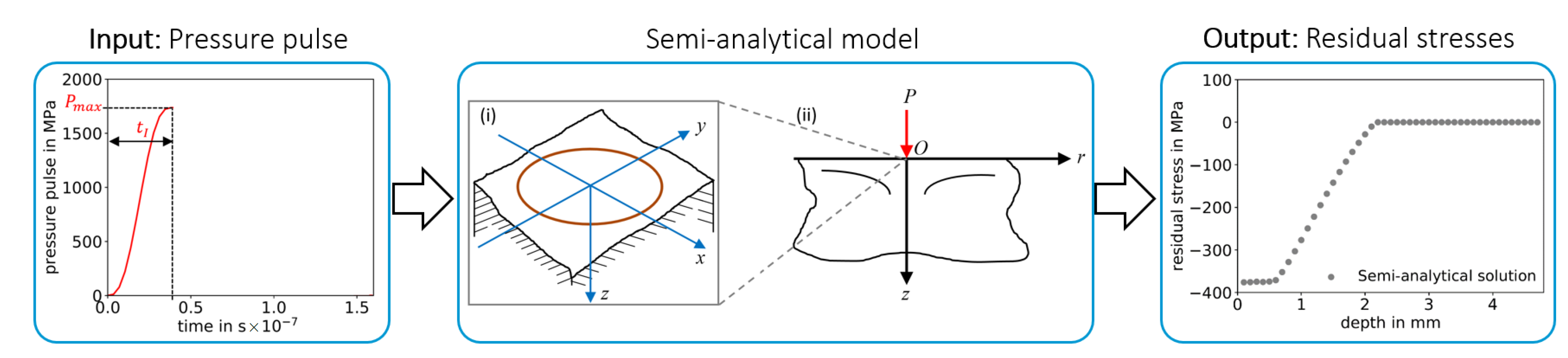
Figure 2.
Illustration of the semi-analytical model by Hu et al. [
23] for computing residual stresses induced by pressure pulse from
Figure 1. Circular pressure pulse area (i) (in red) on the half-space model, which is simplified in (ii) as a concentrated normal load (in red) in the axisymmetric half-space model. Figures (i) and (ii) are republished with permission of the American Society of Mechanical Engineers ASME from [
23].
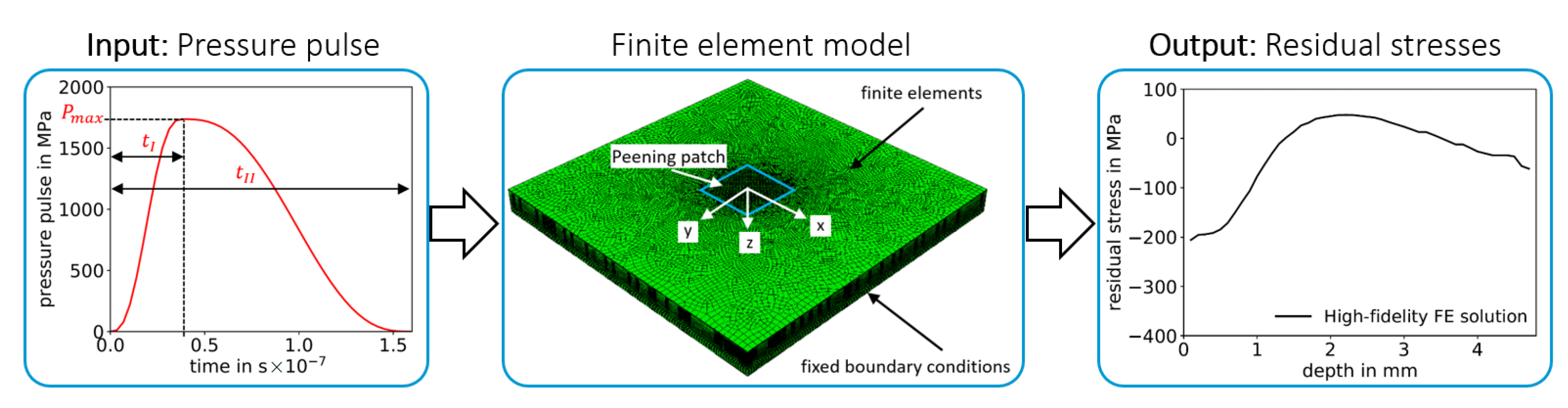
Figure 3.
Finite element process model for computing residual stresses induced by pressure pulse from
Figure 1.
Figure 3.
Finite element process model for computing residual stresses induced by pressure pulse from
Figure 1.
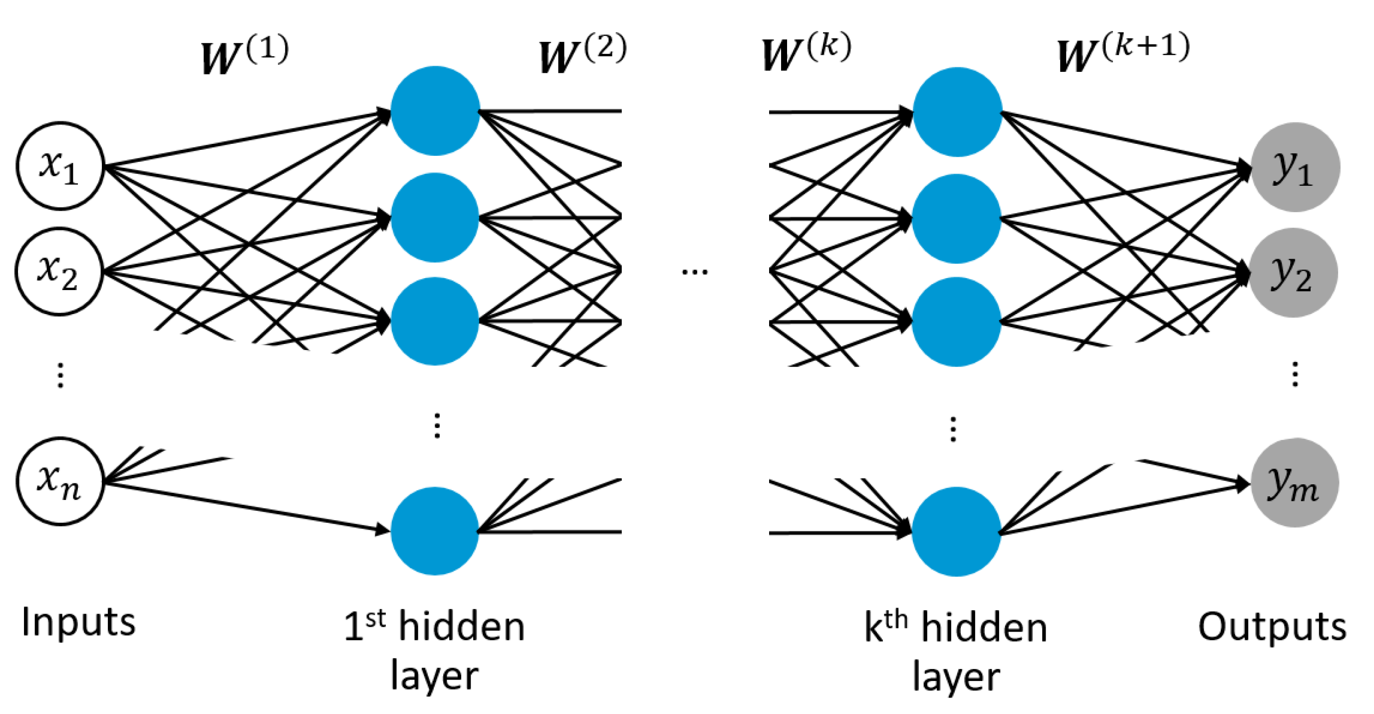
Figure 4.
Schematic of a multi-layered neural network with input layer, k hidden layer and output layer, including weight vectors of edge connections between neurons of adjacent layers for correlating n number of inputs to m number of outputs .
Figure 4.
Schematic of a multi-layered neural network with input layer, k hidden layer and output layer, including weight vectors of edge connections between neurons of adjacent layers for correlating n number of inputs to m number of outputs .
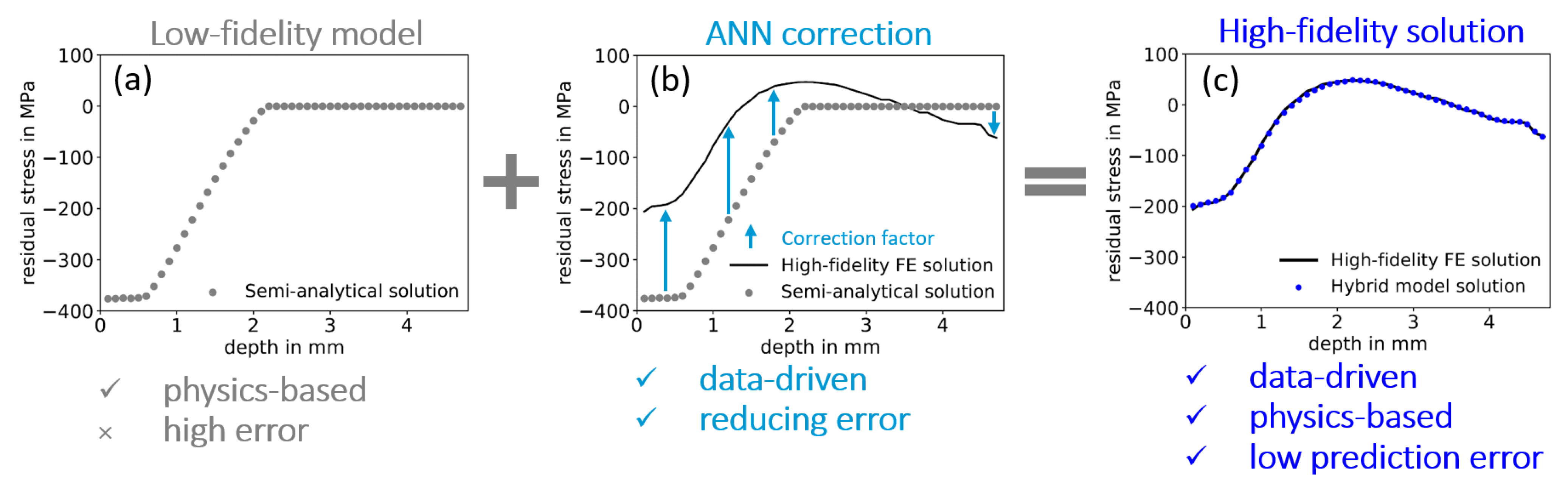
Figure 5.
Schematic of hybrid model implementation for prediction of laser shock peening (LSP)-induced residual stresses: (a) Residual stresses predicted by the semi-analytical model exhibiting relatively high prediction errors compared to the high fidelity FE solution which is compensated by (b) a correction factor “learned” by an artificial neural network (ANN), leading to (c) the validated high-fidelity prediction with low errors, i.e., the hybrid model solution.
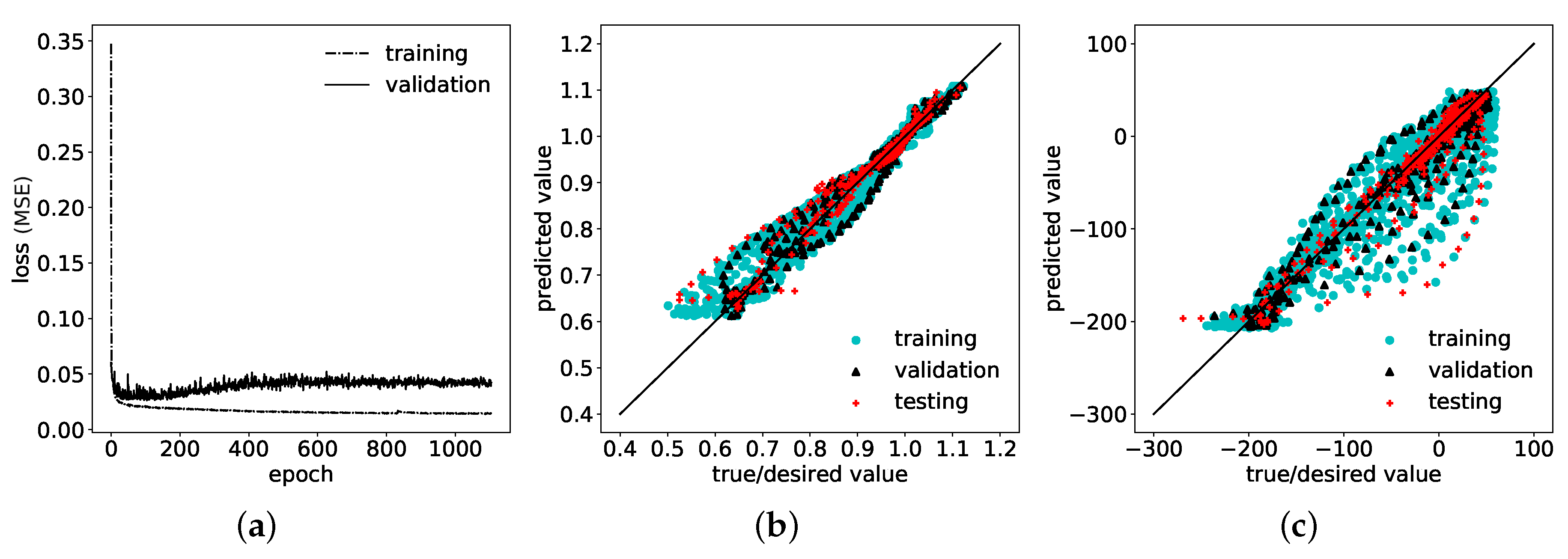
Figure 6.
(a) Learning curves: Mean squared error (MSE)-loss function values minimized via weight adjustment of the ANN on training set and simultaneous MSE for predictions on validation set with training-set weights over number of epochs during training. (b) Determination coefficient for correction factor (ANN output) achieved by ANN on training, validation and test data sets. (c) Determination coefficient for related residual stresses attained by ANN on training, validation and test data sets.
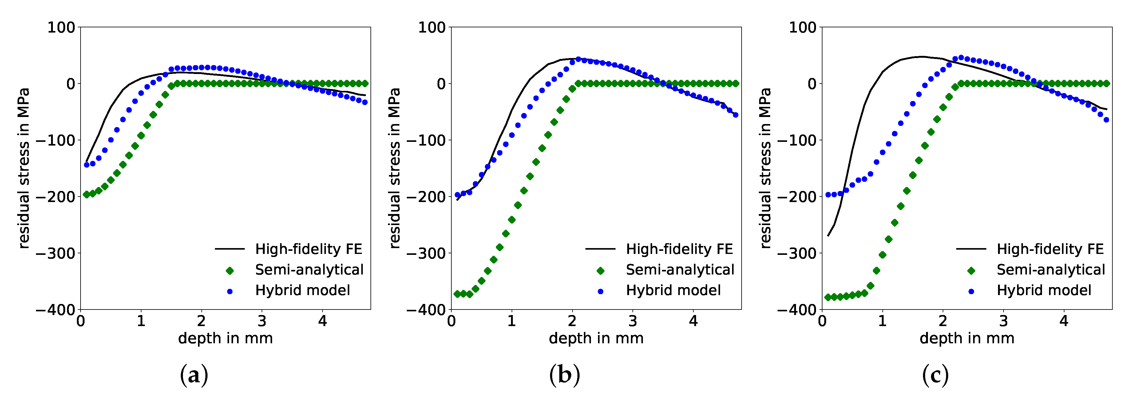
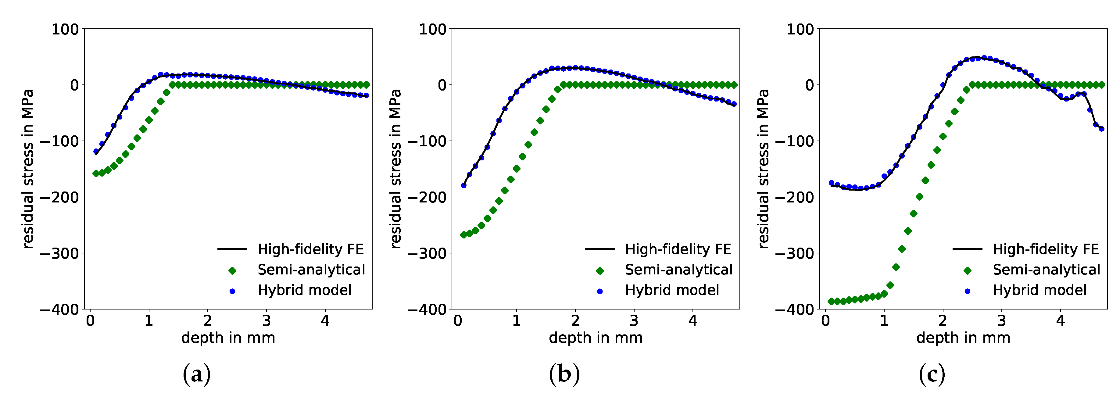
Figure 7.
Comparison of residual stress distributions over depth predicted by the FE model, semi-analytical model and hybrid model for three exemplary test samples with pulse parameters maximum pressure , time of maximum pressure and pulse duration of (a) 1236 MPa, 15.1 ns, 85 ns; (b) 1639 MPa, 37.7 ns, 145 ns; and (c) 1820 MPa, 13 ns, 65.7 ns.
Figure 8.
(a) Super-imposed but indistinguishable residual stress distributions over depth predicted by the semi-analytical model for different pressure pulses, i.e., identical inputs for the corrective ANN-model. (b) Corresponding output targets: Eight unique residual stress distributions over depth predicted by the FE model and (c) corresponding distinctive pressure pulses over time that were used as input for both models, exhibiting different pulse durations but identical maximum pressures and times of respective maximum pressures.
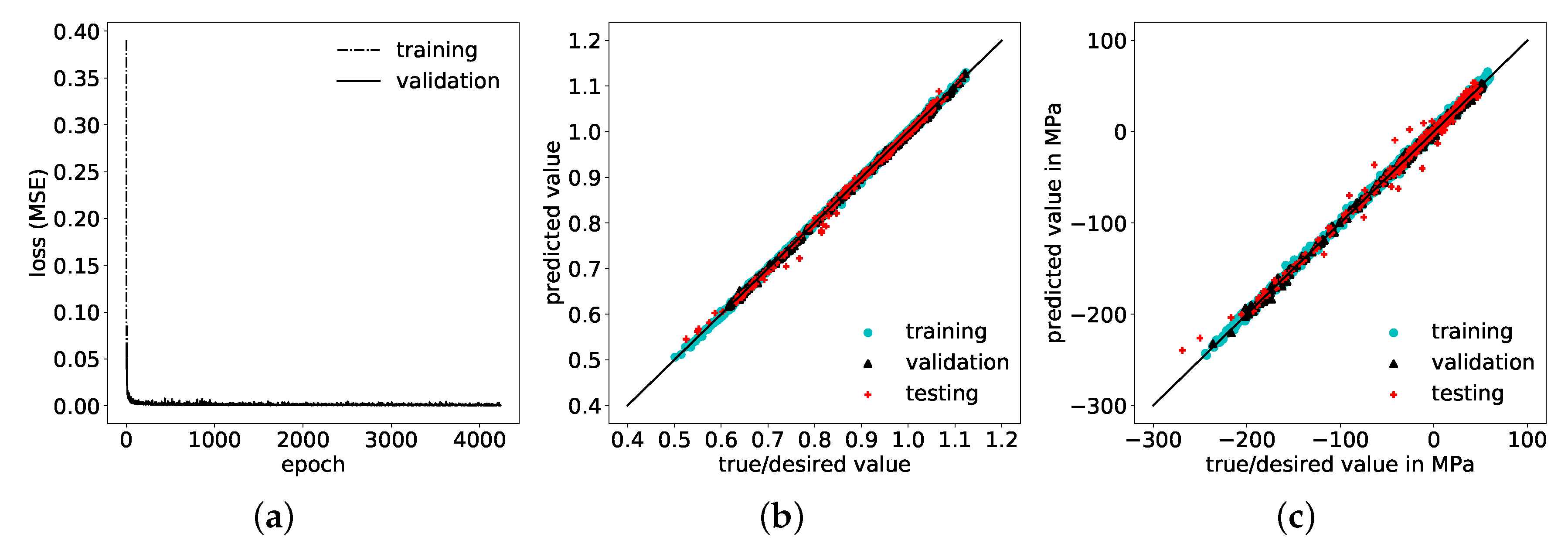
Figure 9.
(a) Learning curves: MSE-loss function values on training and validation data sets over number of epochs during training and (b) corresponding prediction values of the correction factor versus true values, and of (c) the corresponding residual stresses.
Figure 9.
(a) Learning curves: MSE-loss function values on training and validation data sets over number of epochs during training and (b) corresponding prediction values of the correction factor versus true values, and of (c) the corresponding residual stresses.
Figure 10.
Comparison of residual stress distributions over depth predicted by the FE model, semi-analytical model and hybrid model for three test samples with maximum pressure , time of maximum pressure and pulse duration of (a) 1144 MPa, ns, 137 ns; (b) 1390 MPa, ns, 140 ns; and (c) 2039 MPa, ns, 243 ns, respectively.
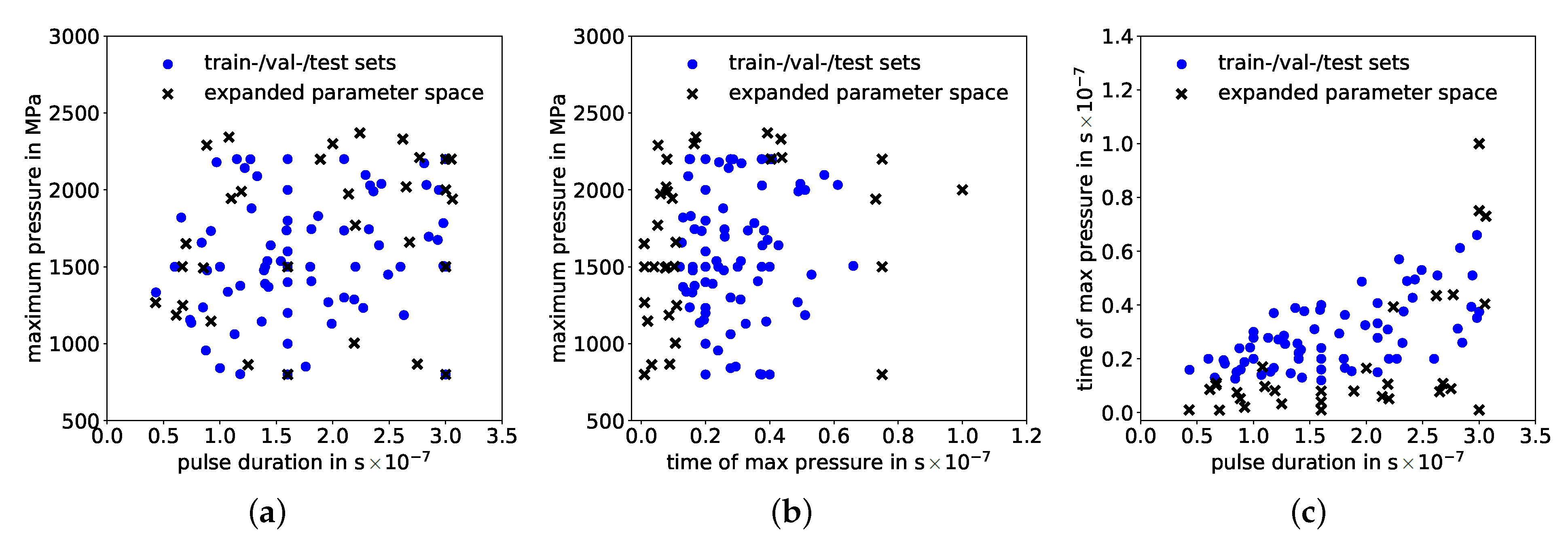
Figure 11.
Sample positioning in the expanded parameter space: Maximum pressure over (a) pulse duration and over (b) time of maximum pressure as well as (c) time of maximum pressure over pulse duration.
Figure 11.
Sample positioning in the expanded parameter space: Maximum pressure over (a) pulse duration and over (b) time of maximum pressure as well as (c) time of maximum pressure over pulse duration.
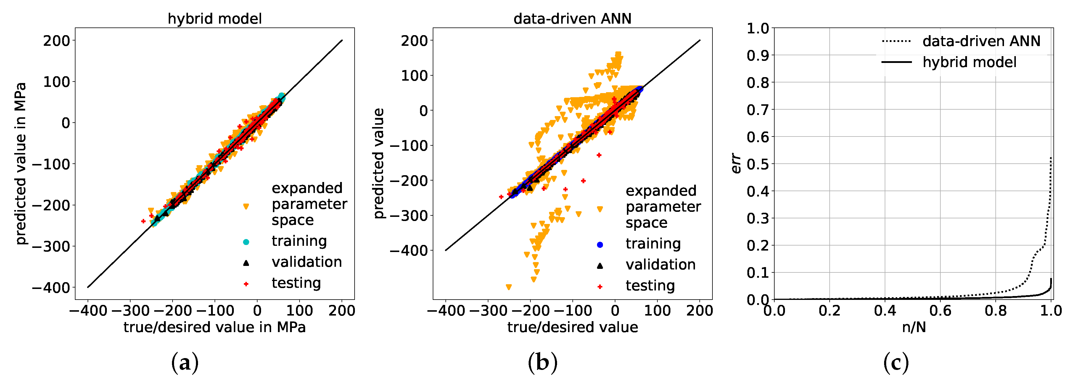
Figure 12.
Juxtaposition of predicted values and true/desired values on training, validation, test sets and expanded parameter space data set, achieved by (a) the physics-based hybrid model and (b) the purely data-driven ANN, respectively. (c) shows the relative error of samples n normalized with the total number of samples N, sorted from low to high values on the data set with expanded parameter space generated by hybrid model and data-driven ANN.
Figure 13.
Comparison of prediction performances of hybrid model and direct ANN with respect to the average mean squared error (MSE) and standard deviation achieved on (a) the test data set and (b) the extrapolation data set, while reducing the amount of the total data set (training, validation and test data sets) from 100% to 20% in increments of 10%-steps, respectively. All MSE average values and standard deviations are based on three different MSEs and their respective standard deviations that are achieved on dissimilar data splits implemented by changing pseudo-random-states.
Table 2.
Pressure pulse parameter ranges of maximum pressure , time of maximum pressure and pulse duration for training, validation and test data sets.
Table 2.
Pressure pulse parameter ranges of maximum pressure , time of maximum pressure and pulse duration for training, validation and test data sets.
| | [MPa] | [ns] | [ns] |
|---|
| Min. | 800 | 12 | 43 |
| Max. | 2200 | 66 | 300 |
Table 3.
Prediction metrics of trained ANN via Approach 1: (determination coefficient) and MSE (mean squared error) for correction coefficients as well as for corresponding residual stresses on training, validation and test data sets, respectively.
Table 3.
Prediction metrics of trained ANN via Approach 1: (determination coefficient) and MSE (mean squared error) for correction coefficients as well as for corresponding residual stresses on training, validation and test data sets, respectively.
| | Correction Factor | Residual Stresses |
|---|
| Data Set | in % | | in % | in MPa |
|---|
| Training | | | | |
| Validation | | | | |
| Test | | | | |
Table 4.
Prediction metrics of the trained ANN via Approach 2: Determination coefficient and MSE for correction coefficients as well as corresponding residual stresses achieved on training, validation and test data sets, respectively.
Table 4.
Prediction metrics of the trained ANN via Approach 2: Determination coefficient and MSE for correction coefficients as well as corresponding residual stresses achieved on training, validation and test data sets, respectively.
| | Correction Factor | Residual Stresses |
|---|
| Data Set | in % | | in % | in MPa |
|---|
| Training | | | | |
| Validation | | | | |
| Test | | | | |
Table 5.
Expanded pressure pulse parameter ranges of maximum pressure
, time of maximum pressure
and pulse duration
as extrapolated parameter space in comparison to the ranges in the data set used for training, validation and testing, see
Table 2.
Table 5.
Expanded pressure pulse parameter ranges of maximum pressure
, time of maximum pressure
and pulse duration
as extrapolated parameter space in comparison to the ranges in the data set used for training, validation and testing, see
Table 2.
| | | in MPa | in ns | in ns |
|---|
| Training, validation, test | Min. | 800 | 12 | 43 |
| Max. | 2200 | 66 | 300 |
| Expanded parameter space | Min. | 800 | 1 | 43 |
| Max. | 2400 | 100 | 306 |
Table 6.
Prediction metrics of the hybrid model and purely data-driven ANN: and MSE for residual stresses of samples in training, validation, test and expanded parameter space data sets.
Table 6.
Prediction metrics of the hybrid model and purely data-driven ANN: and MSE for residual stresses of samples in training, validation, test and expanded parameter space data sets.
| | Hybrid Model | Data-Driven ANN |
|---|
| Data Set | in % | | in % | in MPa |
|---|
| Training | | | | |
| Validation | | | | |
| Test | | | | |
| Expanded space | | | | |


