2.1. Instrumented Indentation Testing
While many implementations of IIT exist, they all involve an indentation process during which a shaped indenter is brought into contact with the material of interest through one or more load and unload cycles. The normal force and displacement are recorded throughout the indentation process, and the tested materials’ mechanical properties are estimated from the load-depth response. As described in the international standard governing IIT [
27], IIT sets itself apart from traditional hardness testing through this continuous recording of load and depth. Doing so enables extraction of a multitude of mechanical properties and obviates the need for subsequent optical inspection of the indent.
The Frontics AIS 2100 IIT instrument, which was originally developed by engineers at Seoul National University (SNU, Seoul, Korea) (see [
28,
29,
30,
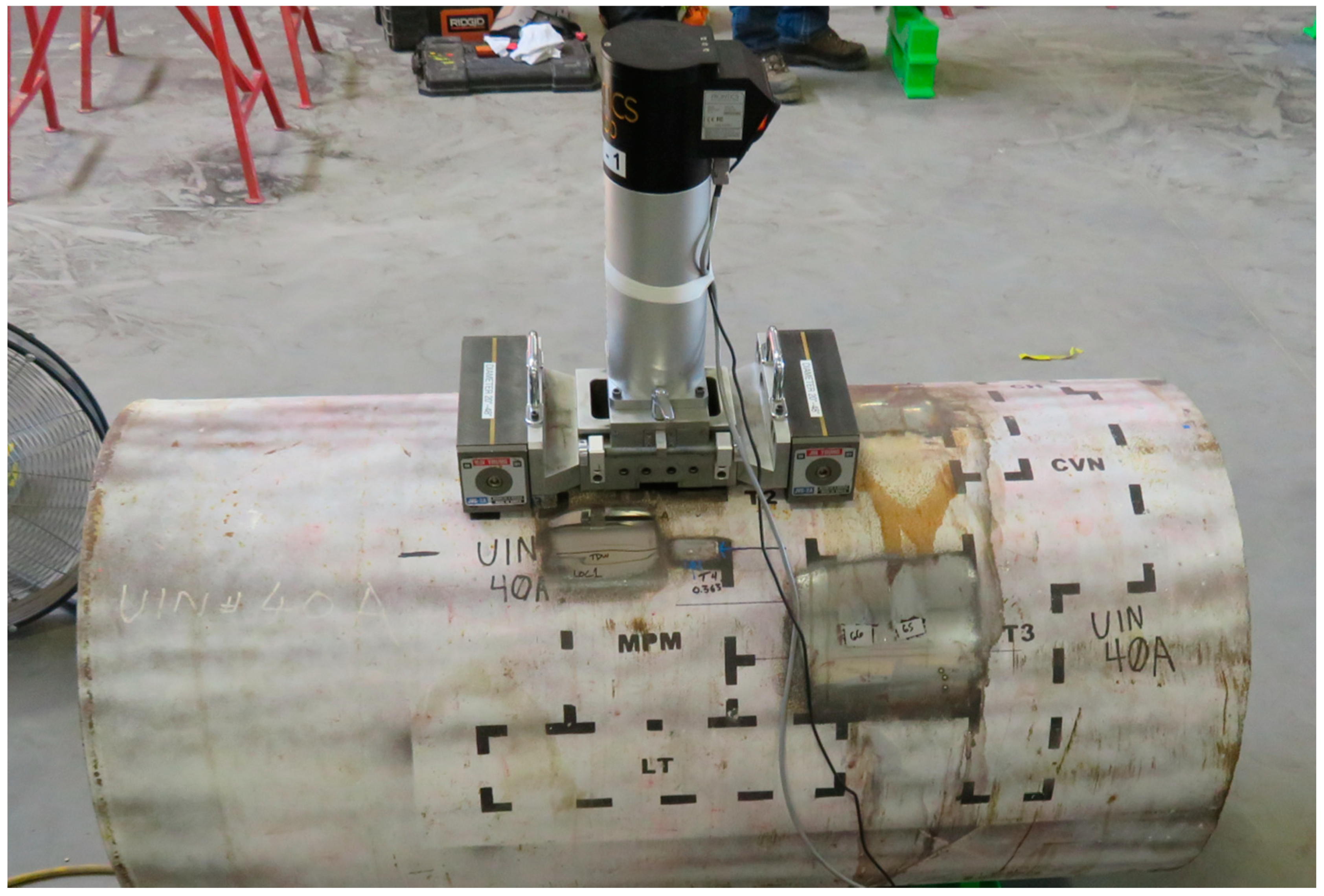
31]), was used in this work, and their loading scheme, as described below, was adopted. This tool employed a 0.5-mm diameter spherical indenter. A photograph of the Frontics AIS 2100 tool, mounted to a pipe sample, is shown in
Figure 1. The instrument is shown mounted to a 24-inch diameter (61-cm; note that the pipelines tested in this effort were manufactured in the United States according to imperial units of measure) pipe by means of a magnetic mounting stand; the instrument was secured to the stand on flat ground, and then, the whole fixture was secured to the pipe by engaging the magnets. For pipes with outer diameters (OD) between 8 and 24 inches (20 and 61 cm), the instrument is mounted via a heavy-duty roller chain that is tightened to a specific torque. Secure mounting of the instrument is critical to ensure a sufficiently stiff test setup.
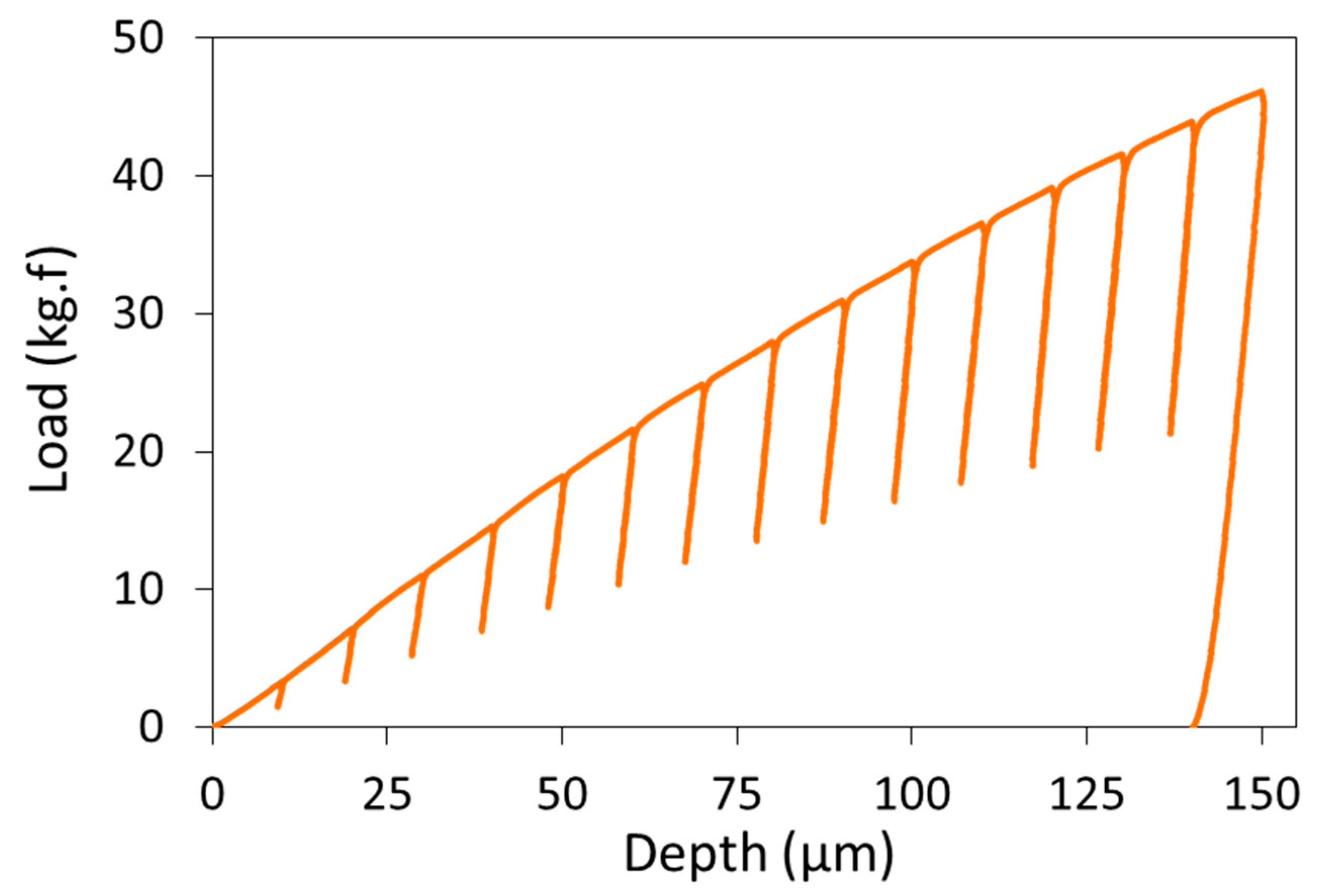
The tool was operated in displacement control and indented the sample surface to a maximum depth of 150 μm, through a series of 15 sequential load/partial-unload cycles, in increments of 10 μm. In each cycle, the indenter reached its target depth (e.g., 50 μm during the 5th load cycle) and unloaded to 50% of the force, corresponding to the target depth, before commencing the next load cycle and re-loading to the next target depth (e.g., 60 μm). As described below, these 15 discrete points of the load-depth response are used to obtain the stress and strain at these times, as well as the complete work hardening response. The resulting load-depth curve, at the conclusion of 15 cycles from a representative IIT measurement, is depicted in
Figure 2.
The algorithm for extracting stress and strain, and subsequently YS and UTS, from this load-depth response is detailed in [
28] through [
31], and it is presented here in summary form. However, it is noted that those authors also relied on the pioneering work of Tabor [
32].
The representative stress of indentation,
, is a function of the applied load,
, and the projected contact area of the indentation,
, as shown in Equation (3).
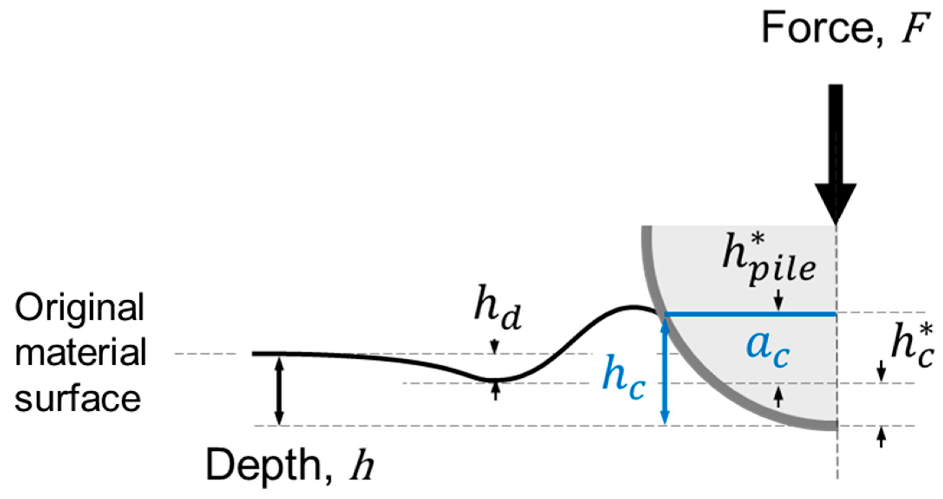
can be calculated from the chordal radius
of the indentation (see Equation (4) and
Figure 3).
is assigned a value of 3.0 based on the work of Jeon et al. [
30].
The representative strain,
, is calculated according to Equation (5), in which the coefficient,
, is assigned a value of 0.14 based on experiments and analysis. It is worth mentioning that this equation, published in [
28,
30], differs from the relationship first proposed by Tabor in [
32].
Equations (1) through (3) introduce new unknowns: the contact radius
, and the contact depth
. These parameters, themselves, are difficult to measure directly in-situ and are, therefore, estimated afterwards from other measured quantities through an empirical model. The detailed procedure for extracting mechanical properties from the indentation response is presented in [
28,
31]. In brief, a power-law stress-strain relationship is assumed (Equation (6)), and the strain hardening exponent
is empirically related to the pile up around the indenter through Equation (7).
The numerical values of the parameters appearing in Equation (7) were established in [
29] through numerical calibration of the IIT algorithm on a range of metallic materials. These parameters are presented here in
Table 1.
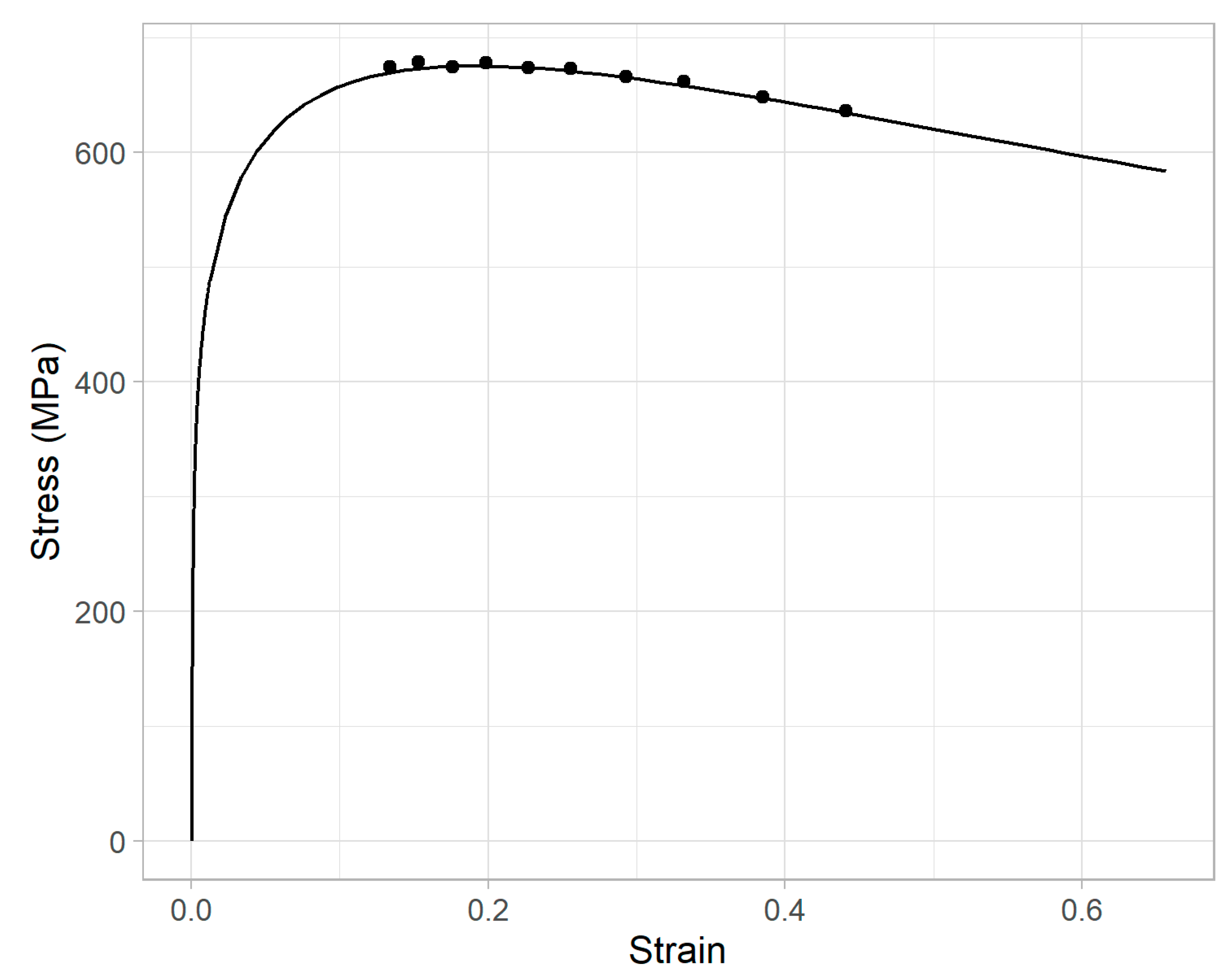
An initial trial value for the hardening exponent n is assumed and used to update the contact parameters and through Equation (7). This new ratio subsequently changes the estimated representative stress and strain ( and ) at the 15 load maxima points from the IIT measurement. A power-law is fit to the final 10 of these updated points, and the process is repeated until the exponent n converges. Note that only the final 10 of the 15 stress-strain points are used in this study since, from the authors’ experience, the first 5 exhibit greater variability due to the very small loads achieved in those load cycles.
The instrument records the time of each instance of load and depth, and therefore, the strain rate can be established from the strain at the 10 discrete points. While the rate varies depending on strains achieved in each test, the typical strain rate over the final 10 of the 15 load maxima was between and . This rate, however, is not fully analogous to the strain rate under uniaxial tensile loading. First, in general, the state of strain beneath the indenter in an IIT test is compressive and multiaxial. Second, the strains achieved just beneath the indenter during IIT exceed the strains reached in tensile tests due to the early onset of necking in tensile tests.
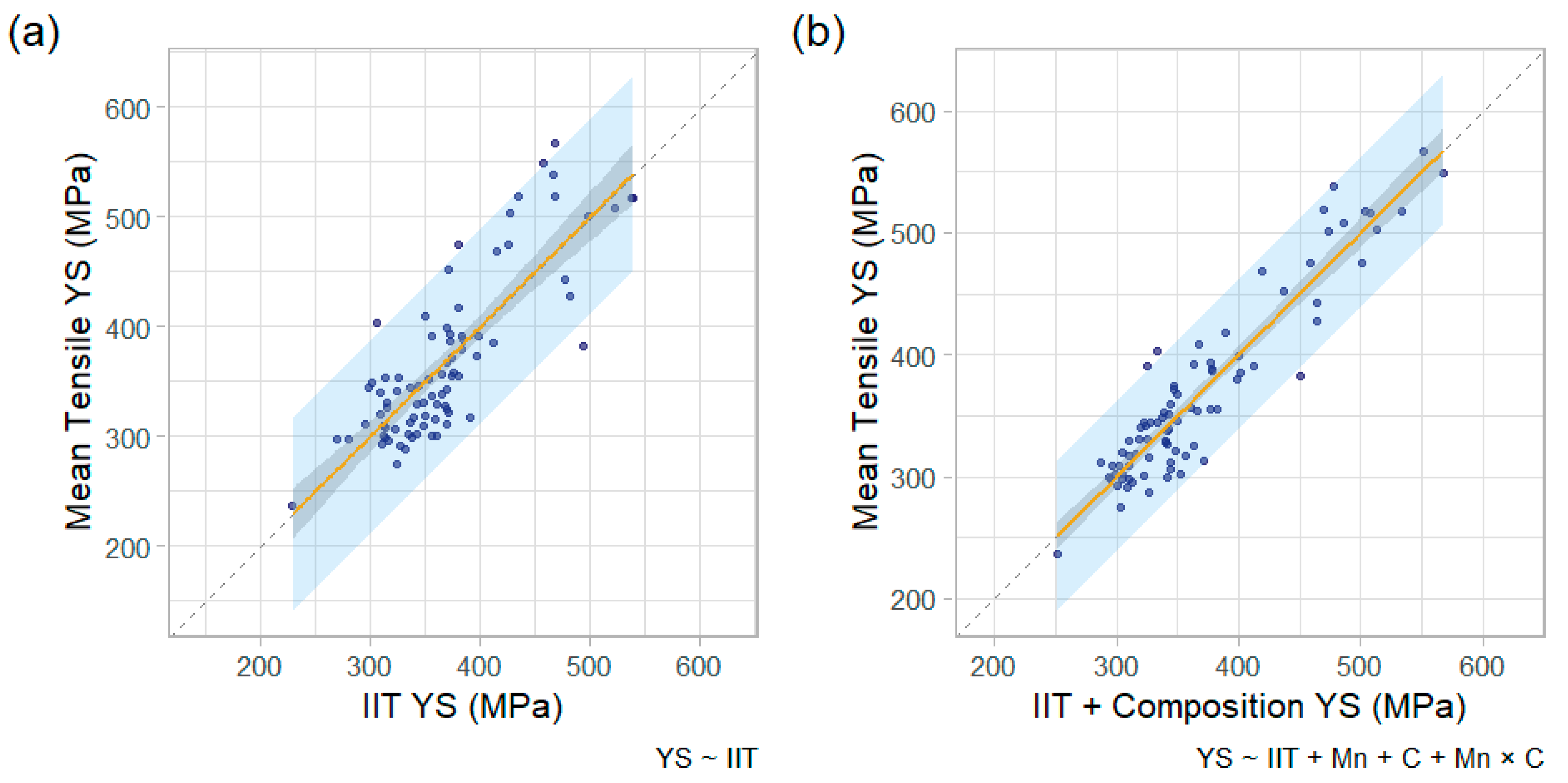
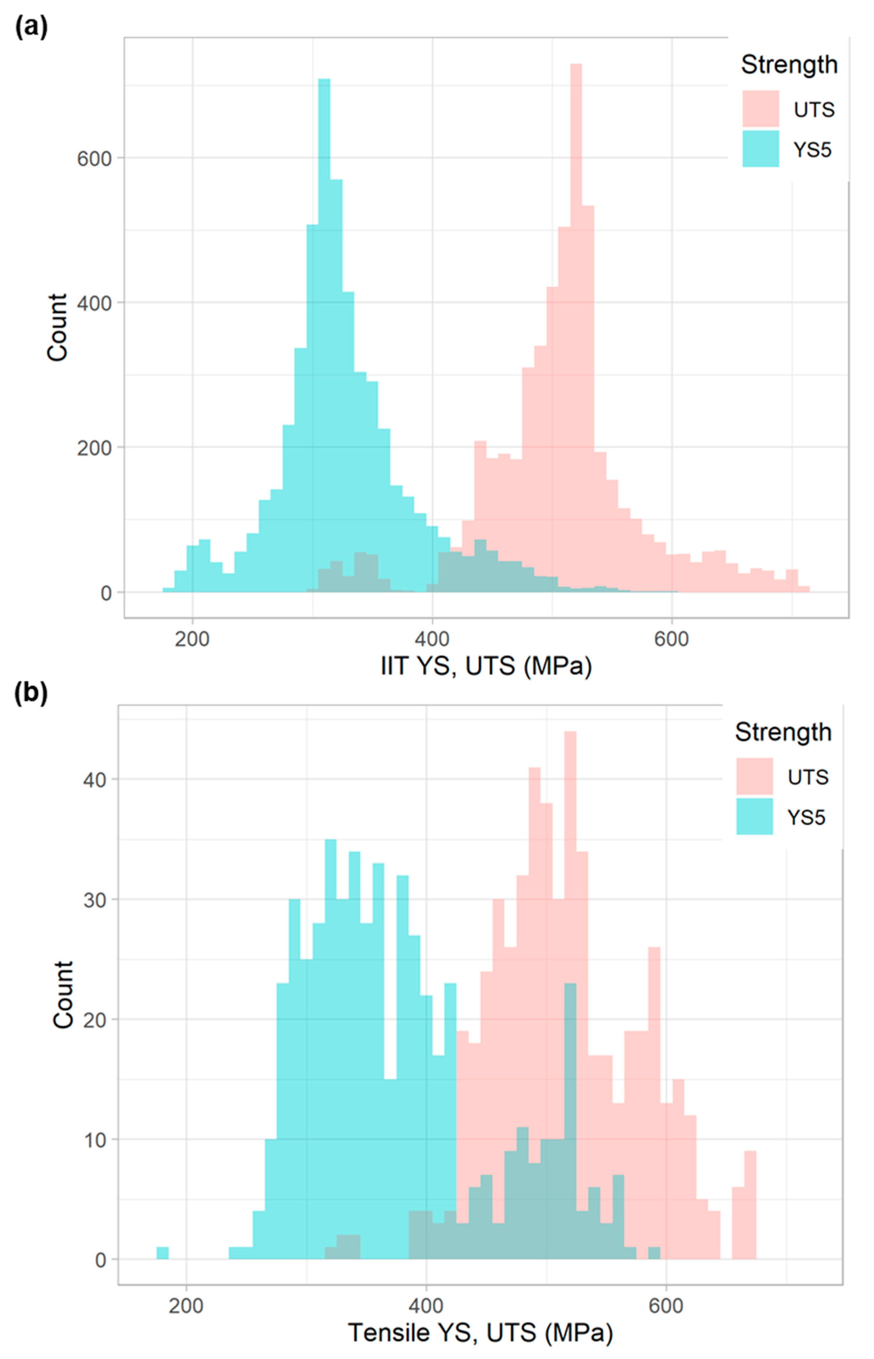
YS and UTS are then computed from the power-law stress-strain curve. In this work, YS is defined as
where YS, corresponding to a total strain of 0.5%, is consistent with the definition adopted for line pipe steels in [
2]. This definition of YS has an advantage over alternatives, such as the 0.2% offset yield stress, in that it can be computed without first measuring Young’s Modulus. By the same token, this definition is only acceptable for materials with Young’s Modulus within a certain range—for example, some aluminum alloys may not have begun to yield at 0.5% strain. However, for the line pipe steels under consideration in this work, 0.5% strain is always beyond the elastic limit.
The UTS is taken as the stress at a strain numerically equal to the computed power-law hardening exponent, i.e.,
. This equality is derived from the Considère analysis of an incompressible, power-law material under uniaxial loading. Therefore, this approach assumes the deformation beneath the indenter is approximated by a uniaxial strain state. Thus, with the power-law stress-strain relationship established:
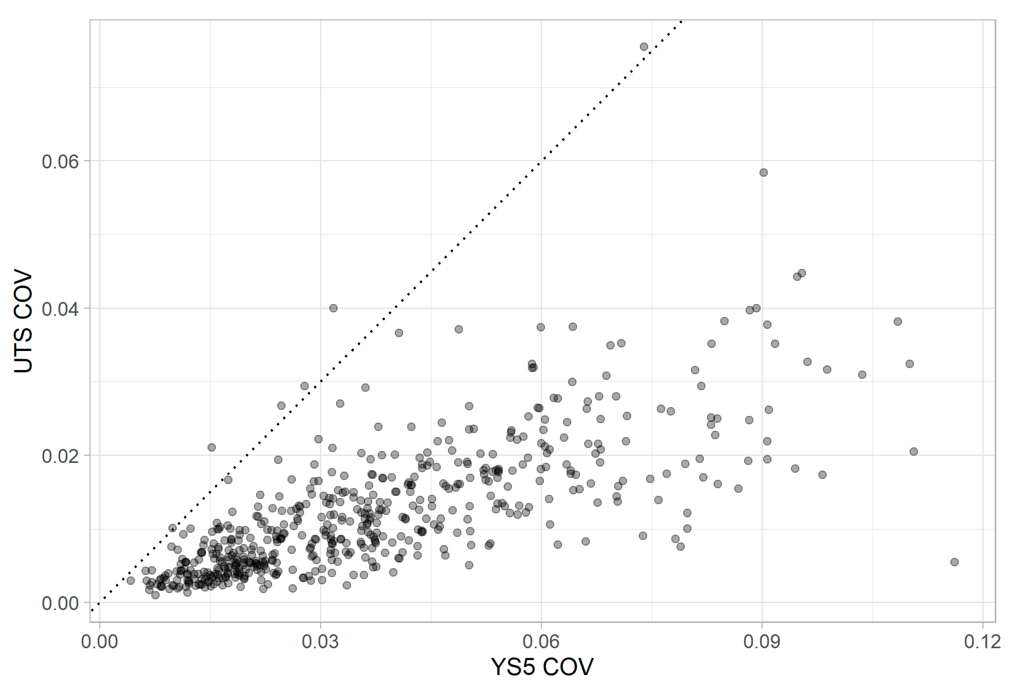
Typically, at least eight measurements, in each of two different locations on the same pipe sample, are taken. This is partly motivated by regulatory requirements [
1], but it is also done to permit detailed analysis of the uncertainty in the technique, which stems from the physical measurements and the iterative IIT algorithm that was adopted. Random error was further mitigated by this replicate sampling.
Through years of experience with this methodology, PG&E has developed several criteria that are used to filter out erroneous measurements. Several of these criteria are detailed in [
33] and include, for example, a method for detecting poor fixturing of the instrument to the pipe by scanning load-depth curves for indications of excessive compliance.
2.4. Materials
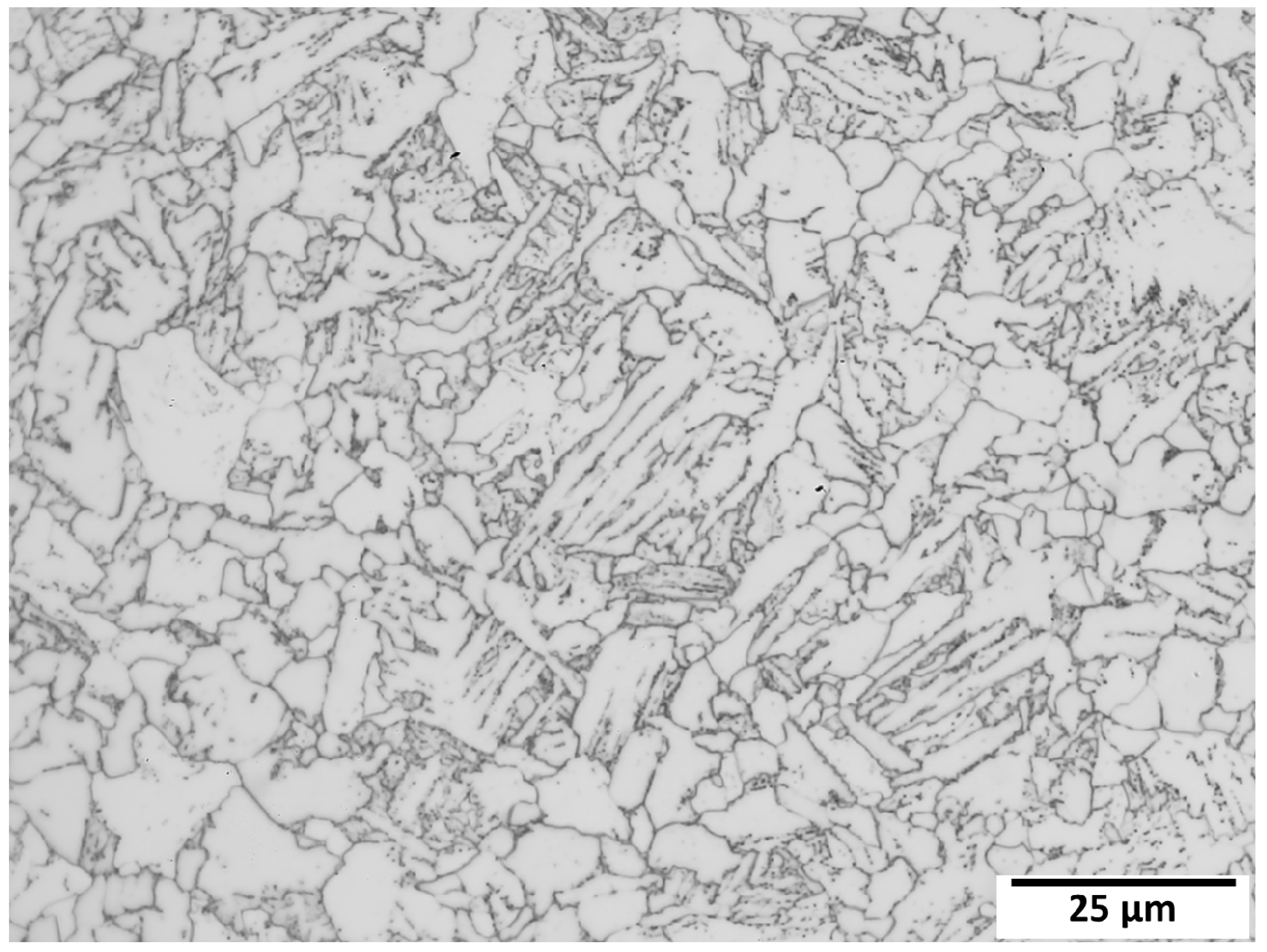
The samples in this study consisted of 197 steel pipe features, including line pipe and fittings. The feature materials included mostly traditional, low-carbon, moderate-strength steel, as well as 3–5 thermomechanically controlled processed (TMCP) steel pipes and 3–5 quenched and tempered (Q&T) steel pipes. As will be described below, the carbon content ranged from about 0.05% to 0.25% in the steels in this study. YS typically ranged between 275 and 415 MPa (40 and 60 ksi), and UTS was between 415 and 550 MPa (60 and 80 ksi). IIT measurements were obtained on site on either active or decommissioned pipeline segments, ranging in diameter from 10.2 cm (4 in.) to 91.4 cm (36 in.), and wall thickness from 4.8 mm (0.188 in.) to 19 mm (0.75 in.).
Prior to indentation, the pipeline surface was carefully prepared to a “mirror finish.” The surface was ground with successively finer-grit sandpaper, using a handheld mechanical sander to a final pass of 2000 grit. The orientation of the sander, relative to the surface, was changed with each successive pass to mitigate groove-in. This entire process is designed to remove a minimum of 10 μm of wall thickness from the OD and, therefore, minimize the presence of any decarburization layer that may exist in the pipe sample.


