Article

Vapor Pressure versus Temperature Relations of Common Elements

1
Department of Materials Science and Engineering, The Pennsylvania State University, University Park, PA 16802, USA
2
Department of Engineering Science and Mechanics, The Pennsylvania State University, University Park, PA 16802, USA
*
Author to whom correspondence should be addressed.
Materials 2023, 16(1), 50; https://doi.org/10.3390/ma16010050
Submission received: 24 November 2022 / Revised: 17 December 2022 / Accepted: 19 December 2022 / Published: 21 December 2022

Abstract

:
The vapor pressure values of common elements are available in the literature over a limited temperature range and the accuracy and reliability of the reported data are not generally available. We evaluate the reliability and uncertainty of the available vapor pressure versus temperature data of fifty common pure elements and recommend vapor pressure versus temperature relations. By synthesizing the vapor pressure values from measurements reported in the literature with the values computed using the Clausius Clapeyron relation beyond the boiling point, we extend the vapor pressure range from 10−8 atm to 10 atm. We use a genetic algorithm to optimize the fitting of the vapor pressure data as a function of temperature over the extended vapor pressure range for each element. The recommended vapor pressure values are compared with the corresponding literature values to examine the reliability of the recommended values.

1. Introduction

The vapor pressures of elements at various temperatures are important for a wide range of scientific and engineering calculations [1,2,3,4,5,6]. Vapor pressure data are important for many metal processing operations and properties of many alloys. They are needed to predict the loss of alloying elements due to vaporization during additive manufacturing and fusion welding and for the deposition of various thin films of commercial interest [1,2,3,4,5,6]. In the keyhole mode welding and additive manufacturing processes, the relationship between temperature and vapor pressure is a requisite to predict the shape, size, and stability of the keyhole [7]. Similarly, in the pyrometallurgical production of metals, vapor pressure and the rates of evaporation of zinc and cadmium are used in the final refining steps of their extraction [8,9]. Accurate knowledge of the vapor pressure is necessary to have a vapor coating of elements [10]. In high-pressure systems such as nuclear reactors, the choice of coolants like liquid sodium or alloys of sodium-potassium and lead-bismuth is affected by their vapor pressures [11]. Therefore, an accurate database of vapor pressure for elements is needed for different scientific and technological applications.
Despite the importance of vapor pressure data, work on the vapor pressure of elements has not advanced much since the 1980s when Hultgren compiled the vapor pressure data of several elements [12]. These vapor pressure data at various temperatures were fitted by Alcock et al. [13] and Gale et al. [14], using linear regression to provide relations between vapor pressure and temperature. However, for most elements, the resulting fitted equations are valid for a narrow temperature range much below the boiling point of the liquid. For example, for Vanadium with a boiling point of 3680 K, the vapor pressure equation from Smithells Metals Handbook is only valid till 2175 K leaving a temperature range of 1505 K below the boiling point with no vapor pressure-temperature data. The second major issue is that these sources provide multiple equations to represent the change in vapor pressure for different temperature ranges. For example, while Gale et al. [14] uses two equations for several elements, Alcock et al. [13] uses two equations for each element. Finally, for several elements, the temperature which corresponds to 1 atm pressure does not match the boiling point of the elements. For example, in the case of calcium, the predicted boiling point using the Gale et al. [14] relation differs from the literature boiling point by 100 K. What is needed and currently not available are vapor pressure values of elements over a wide range of temperatures and the reliability and uncertainty of the data.
We seek to develop a single vapor pressure-temperature relation valid for a wider temperature, i.e., up to a maximum pressure of 10 atm which can also correctly predict the boiling point of the element. This work uses the experimental data reported in the literature and synthesized data using Clausius Clapeyron relation to represent vapor pressure over a large range of temperatures for fifty elements. For each of the fifty elements, the resulting vapor pressure versus temperature data was fitted into an equation. The fitting of the vapor pressure versus temperature data was optimized using a genetic algorithm (GA) and the accuracy of the fitting was evaluated. Finally, the reliability of the recommended pressure versus temperature relation was examined by comparing the recommended values with the corresponding values reported in the literature.

2. Methodology

The experimental data of vapor pressure versus temperature were collected from the literature and where data were not available, the Clausius Clapeyron thermodynamic relation was used to fill in the gaps in the available data. The resulting data were fitted to an equation for each element. The data fitting was optimized using a differential evolution (DE) algorithm [15,16,17]. The methods of data collection and data fitting optimization are discussed below.

2.1. Data Collection

We collected the vapor pressure data ranging from 10−8 atm (1.013 × 10⁻³ Pa) to 10 atm (1.013 × 10⁶ Pa). The data at low pressure and temperatures below the boiling point are available in the literature [12]. These data were collected for all fifty elements [12]. The lowest pressures for which data was collected [12] is 10−8 atm because this pressure corresponds to the ultra-high vacuum achieved by most commercial equipment [18]. At high temperatures, vapor pressure data are not available. We assumed that the vapor behaves as an ideal gas and estimated the vapor pressure using the Clausius-Clapeyron equation [19] as,
ln ( p 1 p 2 ) = Δ H v a p R ( 1 T 2 1 T 1 )    
where Δ H v a p is the enthalpy of vaporization in J/mol and is assumed to be independent of temperature. P 1 and P 2 are pressures in atm, at temperatures T 1 and T 2 in Kelvin, respectively. Using P 1 as 1 atm and T 1 as the normal boiling point of an element, we calculated the pressure P 2 at temperature- T 2 , the temperature of interest. The symbol R represents the gas constant (8.314 J/mol-K). Thus, vapor pressure data at temperatures above the boiling point were generated. Table 1 lists the boiling point and the enthalpy of vaporization of all fifty elements [20,21]. The vapor pressures were calculated using the Clausius-Clapeyron relationship up to 10 atm. The upper limit of 10 atmospheres is considered to limit the uncertainty of the predicted values.
The collected vapor pressure data ranging from 10−8 atm to 10 atm were used as the input data for a genetic algorithm to determine the coefficients A, B, C, and D of an equation of the following form [13,14],
log ( P ) = A T + B + C   · log ( T ) + 10 3 · D · T    
Here, T has units of Kelvin, and P is pressure in atmospheres. Genetic Algorithm optimizes the values of the four coefficients A, B, C, and D to achieve the best data fitting as discussed below.

2.2. Data Fitting Optimization Using the Differential Evolution Genetic Algorithm

The genetic algorithm (GA) used a differential evolution (DE) method that has been demonstrated in many scientific and technological problems like the determination of the ground state of Si-H crystals [16] and the determination of earthquake hypocenter [17].
Figure 1 shows schematically the various steps of the DE optimization algorithm for each element. First, DE randomly selected an initial population of A, B, C and D. Each of the population contained ten vectors to improve the accuracy of the data fitting. Each vector had four elements corresponding to the four coefficients A, B, C, and D in Equation (2). Next, additional vectors were generated through the process of mutation where an additional mutant vector can be expressed as,
V ( i ) m u t a n t = V j ( i ) + m f · ( V k ( i ) V l ( i ) )    
where V j ,     V k , and V l are random initial population vectors, ‘mf’ is the mutation factor that controls the evolution of the population. The index ‘i’ corresponds to the elements in the vector (coefficients A, B, C, and D).
After the mutation, the mutant vectors were combined with the initial population vector to generate a trial vector. This process is called cross-over. The trial vector was tested against the initial population vector using an objective function represented as,
f = 1 n ( l o g P ( A T + B + C   l o g T + 10 3 D T ) ) 2  
where f is the sum of the squared difference between vapor pressure (P), and the values calculated by the coefficients from the differential evolution algorithm, and ‘n’ is the number of data points. ‘f’ also indicates the fitness value for each population. For the comparison of the initial population vector against the trial vector, the vector with the lowest value of f is kept for the next generation. This comparison is repeated for each vector of the population. When the comparison for all population vectors in a generation was concluded, the process was repeated until the total number of generations was completed. The total number of generations was chosen to be 500,000. The above process was repeated for each of the fifty elements to obtain the coefficients A, B, C, and D. The calculation was done using an in-house FORTRAN code compiled using the Intel® Fortran Compiler, ifort version 2021.7.0.

3. Results and Discussion

3.1. Improved Vapor Pressure Relation

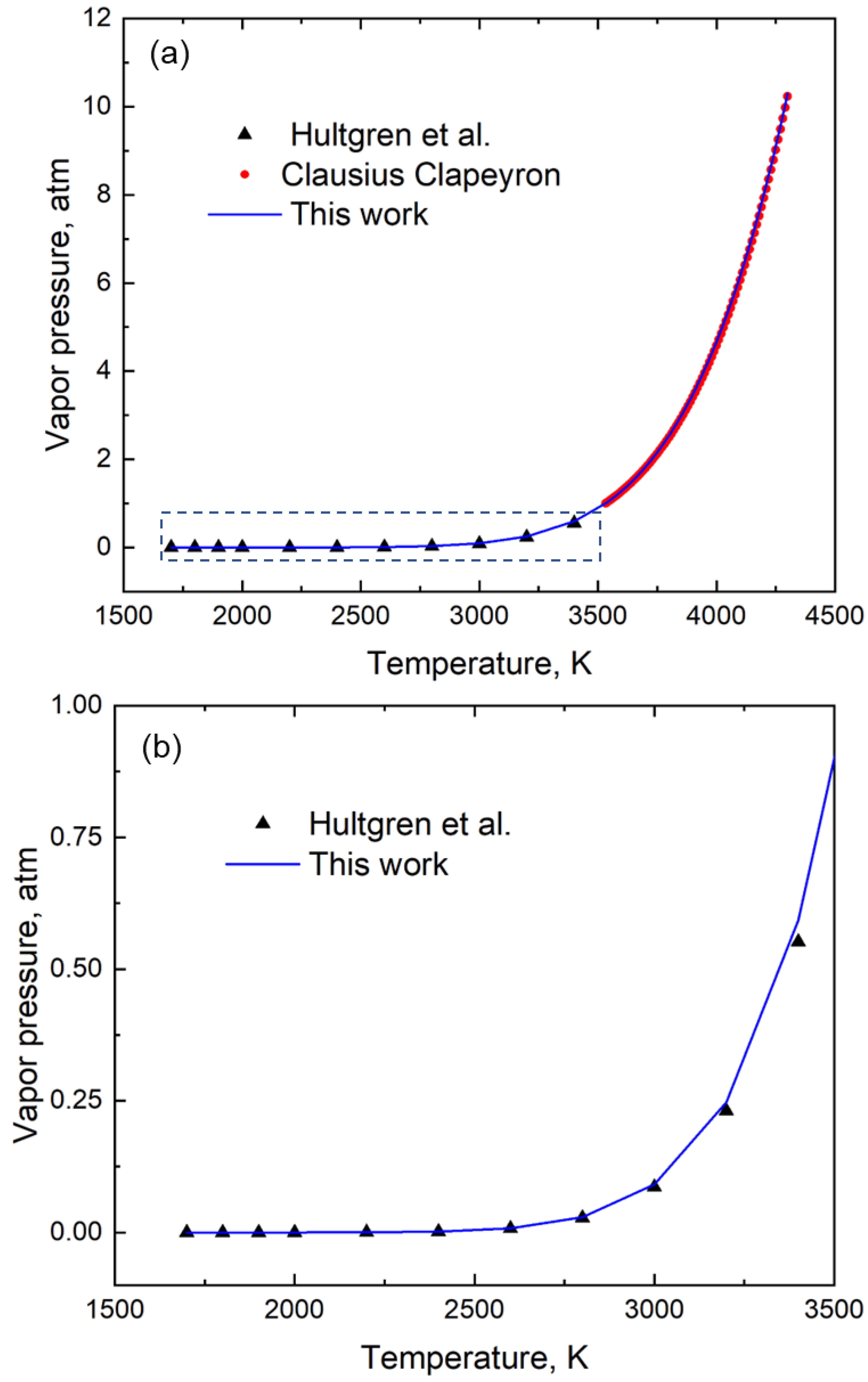
Table 2 reports the coefficients A, B, C, and D of the vapor pressure-temperature relation (shown in Equation (2)) for fifty elements. These coefficients were derived using the genetic algorithm method of optimization as explained earlier. Figure 2 shows an example of the optimization of the fitting using the element silicon. In this figure, the blue line represents the vapor pressure-temperature relation between 1700 K and 4300 K. This blue line is generated from the vapor pressure versus temperature data using its coefficients A, B, C, and D (Table 2) in Equation 2 obtained using a genetic algorithm. The black triangles represent the experimental vapor pressure data between the temperature of 1700 K and 3400 K taken from Hultgren’s handbook [12]. The vapor pressure data synthesized using the Clausius Clapeyron equation and the enthalpy of vaporization and boiling point information [20] is shown by the red circles in the plot (Figure 2). The first red circle represents the boiling point (3533 K) corresponding to 1 atm pressure and the last circle corresponds to a pressure near 10 atm, i.e., a temperature of 4300 K. This combined experimental and synthesized vapor pressure data of Si represented by the black triangles and red circles were used in GA to calculate the coefficients of the equation. The experimental data from Hultgren et al. [12] and the corresponding fitted results using the coefficients of GA is provided in Table A1 of Appendix A. Using the coefficients for element Si, the temperature corresponding to 1 atm pressure is predicted to be the boiling point of the element which is calculated to be 3533 K. The boiling point of Si as reported in the literature [20] is 3533 K. We thus show that our single vapor pressure-temperature relation is valid for a wide temperature while also correctly predicting the boiling point of the element.
To represent the utility of the relation for the entire range of pressure, a root mean square error (RMSE) is provided along with the coefficients in Table 2. RMSE is calculated based on the difference between the vapor pressure versus temperature relation using the optimized coefficients and the pressure that was calculated in data collection stage is represented as
R M S E = 1 n ( P l i t P G A ) 2 n        
where P l i t corresponds to the pressure obtained from literature or using Clausius Clapeyron relation. P G A is the pressure calculated using the coefficients provided by GA and n is the number of data points. RMSE for the fifty elements are provided in Table 2.
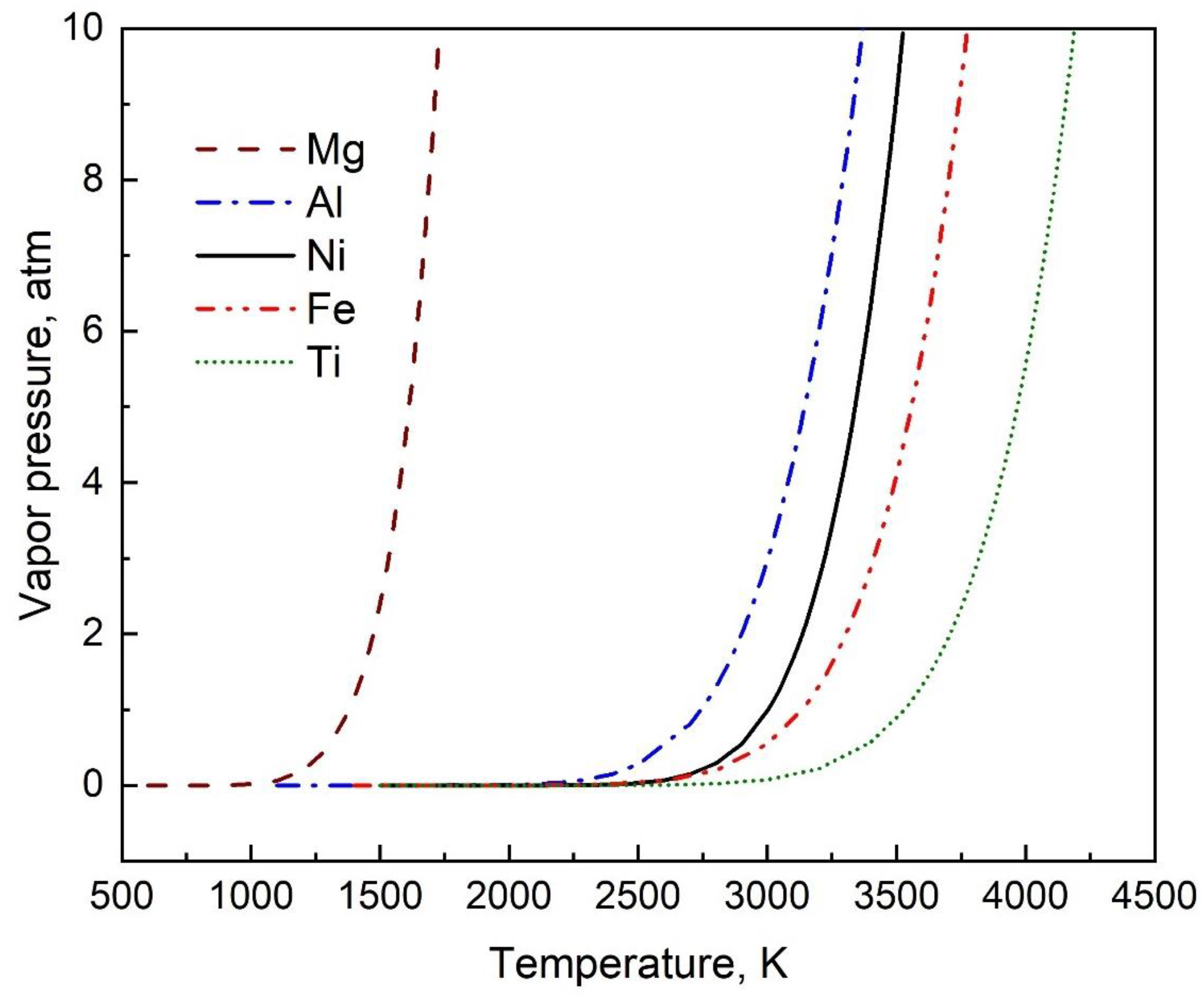
The variation of vapor pressure with temperature for five commonly used elements of Mg, Al, Ni, Fe, and Ti are obtained using the coefficients generated from this study (Table 2) and is shown in Figure 3.
We show that a single relation is sufficient to represent the entire range of vapor pressure even for the elements for which two or more relations were needed. For example, Gale et al. [14] used two equations to define the vapor pressure of Zn between 500 and 1000 K, where one equation was for 473 K to 692.5 K and the other was for 692.5 K to 1000 K. These two relations are represented by the black squares and red circles in Figure 4, respectively. Here, we provide a single equation, represented by the blue line, that can be used to describe the vapor pressure over the entire temperature range of 500 to 1475 K accurately. Thus, the coefficients for Zn derived from GA are valid from 500 K to 1475 K and provide vapor pressure with a mean absolute error of 4.44 × 10⁻⁴ atm (Figure 4).
The average fitness error (F) that represents the soundness of the data fitting by GA for each generation is calculated as
F = 1 N   1 N f  
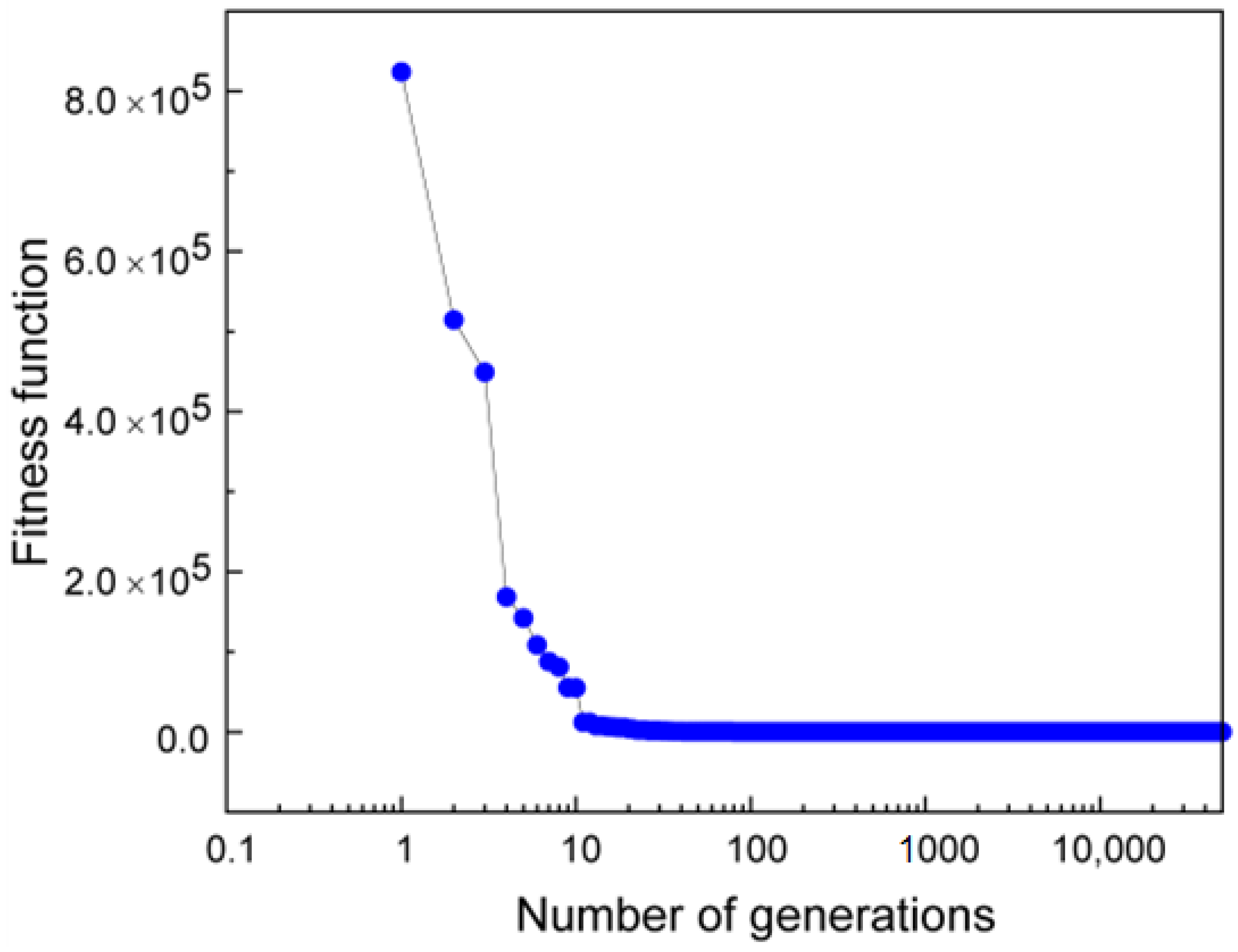
where ‘N’ is the number of populations and ‘f’ is calculated using Equation (4). A plot of the average fitness error as a function of number of generations for Si is shown in Figure 5. Fitness error decreases rapidly from 8 × 10⁵ for the initial population to 922, 16, 0.46, and 0.01 in the 30th, 100th 1000th, and 10,000th generation, respectively, and finally to 0.002 at the end of the 50,000th generation. This indicates that the GA converges rapidly and provides a very good fitting indicated by the low fitness error. The relations provided by GA are tested using independent experimental data as discussed below.

3.2. Verification with Data

To test the results of our approach, independent data (other than the handbook [12]) were also used to examine the accuracy of the relations provided by GA. It is seen that for element Li, the results from GA not only follow the same trend as that reported by Kondo et al. [22], but it can also provide data up to a much higher temperature (Figure 6) with a mean absolute error of 1.25 × 10⁻² atm.

3.3. Quantification of Uncertainty and Reliability of Our Results

Pressure predicted using the coefficients provided by GA is compared with the experimental value. The uncertainty in prediction is represented using the following relation:
U = ( P c a l P e x p ) P e x p × 100  
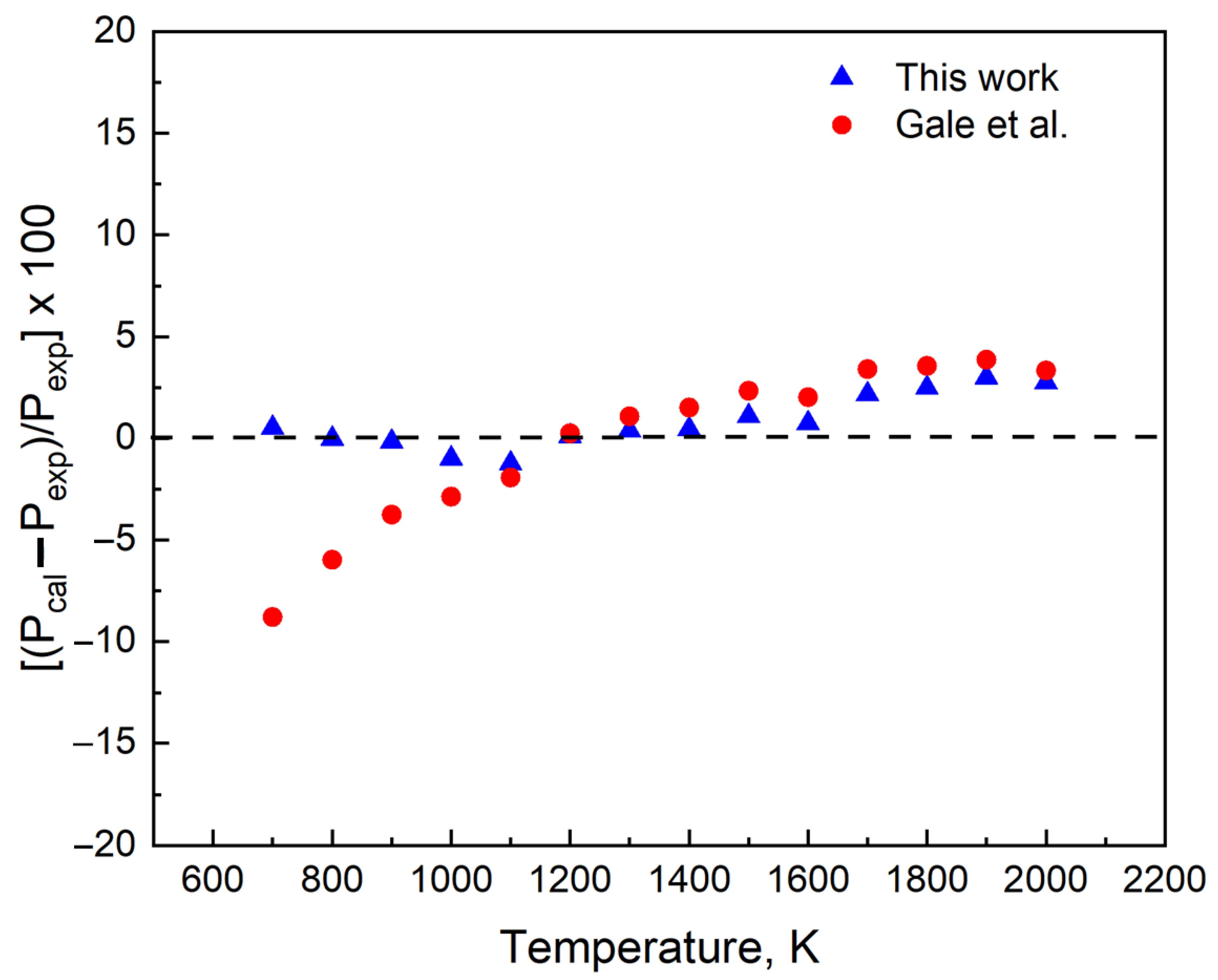
P c a l is the pressure predicted using the coefficients A, B, C, and D in Equation (2) and P e x p is the experimental pressure collected from [12]. Using element Pb as an example (Figure 7), we find that the pressure predicted ( P c a l ) is within 3% of the experimental value.
The reliability of our proposed equation of vapor pressure can be evaluated by comparing the vapor pressure values computed using our equation with the vapor pressure values in the literature. The calculated values of the vapor pressure of Pb (Figure 8) are compared with those computed using the coefficients provided by Alcock et al. [13] and Gale et al. [14]. The data are available between 600 K and 1200 K in Alcock et al. [13]. and from 600 K to 2030 K in Gale et al. [14]. The coefficients are valid between 600 K and 2600 K. Figure 8 shows that our data is within the range of the data available in the literature. Therefore, our data is reliable as well as covers a wider range of temperatures that is not currently available in the literature.

3.4. Sources of Error

GA is a robust tool to fit non-linear, non-differentiable functions, and the accuracy of the fit can depend on various factors such as the number of generations, initial population size, cross-over ratio, and mutation factor. This approach of data fitting using GA may contribute to some errors. We were able to minimize the error from GA by choosing a large number of generations as 50,000. In addition, it is evident from Figure 4 that the fitness error reaches a low value of 0.002 atm at the end of the calculations ensuring a good fit.
Since both experimental data and data from the Clausius Clapeyron relation are used as inputs in GA, incorrect experimental data can also result in errors. Often the experiments for vapor pressure data were not available for high-purity elements. For example, vapor pressure measurements are available for commercially pure elements which often contain impurities. The presence of a substantial level of impurity in the element of interest indicates that the measured vapor pressure may not reflect the correct vapor pressure of the element unless they are corrected [23].

4. Summary and Conclusions

We synthesize vapor pressure data from the literature and use the Clausius Clapeyron relation to provide the vapor pressure versus temperature relations for fifty elements. The relations are applicable for a wide range of temperatures and provide vapor pressure from 10−8 atm (1.013 × 10⁻³ Pa) to 10 atm (1.013 × 10⁶ Pa) with a very low root mean square error in the order of 10−2 atm. We found that the vapor pressure values computed using the relations are consistent with the independent experimental data. In addition, the relations are capable of predicting the boiling points of elements accurately. Finally, the relations are found to be reliable in predicting the vapor pressure with a maximum deviation of 10−3 atm pressure from the existing database.

Author Contributions

Conceptualization, B.M. and T.D.; methodology, B.M.; software, B.M.,T.M., N.W.F., A.S., M.Z.G., T.D.; validation, B.M.,T.M., N.W.F., A.S., M.Z.G.; formal analysis, B.M.,T.M., N.W.F., A.S., M.Z.G.; investigation, B.M., T.M., N.W.F., A.S., M.Z.G.; resources, T.D.; data curation, B.M., T.M., N.W.F., A.S., M.Z.G.; writing—original draft preparation, B.M.; writing—review and editing, B.M.,T.M., N.W.F., and T.D.; visualization, B.M. and T.M.; supervision, T.D.; project administration, T.D., and T.A.P.; All authors have read and agreed to the published version of the manuscript.

Funding

This research received no external funding.

Institutional Review Board Statement

Not applicable.

Informed Consent Statement

Not applicable.

Data Availability Statement

Not applicable.

Conflicts of Interest

The authors declare no conflict of interest.

Appendix A

Table A1 indicates the difference between the experimental data [12] and the fitting results in Figure 2 between 1700 K and 3400 K. The coefficients A = 17,250, B = −15.97, C = 6.403 and D = −0.5281 shown in Table 2 are used in Equation (2) to generate the fitting results. A good agreement between the experimental data and the fitting results is observed.
Table A1. Comparison between the experimental data [12] and the fitting results in Figure 2 between 1700 K and 3400 K.
Temperature, KExperimentally Measured Vapor Pressure, AtmVapor Pressure from the Fitted Equation, Atm
17004.5 × 10−74.67 × 10⁻⁷
18002.15 × 10−62.19 × 10⁻⁶
19008.74 × 10−68.74 × 10⁻⁶
20003.07 × 10−53.06 × 10⁻⁵
22002.7 × 10−42.68 × 10⁻⁴
24000.001640.00165
26000.007520.00773
28000.02780.02902
30000.08620.09114
32000.2310.24713
34000.5520.59291

References

  1. DebRoy, T.; Wei, H.L.; Zuback, J.S.; Mukherjee, T.; Elmer, J.W.; Milewski, J.O.; Beese, A.M.; Wilson-Heid, A.; De, A.; Zhang, W. Additive manufacturing of metallic components—Process, structure and properties. Prog. Mater. Sci. 2018, 92, 112–224. [Google Scholar] [CrossRef]
  2. Ahsan, F.; Ladani, L. Temperature profile, bead geometry, and elemental evaporation in laser powder bed fusion additive manufacturing process. JOM 2020, 72, 429–439. [Google Scholar] [CrossRef]
  3. Mundra, K.; DebRoy, T. Toward understanding alloying element vaporization during laser beam welding of stainless steel. Weld. Res. 1993, 72, 1s–9s. [Google Scholar]
  4. Li, G.; Li, X.; Guo, C.; Zhou, Y.; Tan, Q.; Qu, W.; Li, X.; Hu, X.; Zhang, M.X.; Zhu, Q. Investigation into the effect of energy density on densification, surface roughness and loss of alloying elements of 7075 aluminium alloy processed by laser powder bed fusion. Opt. Laser Technol. 2022, 147, 107621. [Google Scholar] [CrossRef]
  5. Liu, T.; Yang, L.J.; Wei, H.L.; Qiu, W.C.; DebRoy, T. Composition change of stainless steels during keyhole mode laser welding. Weld. J. 2017, 96, 258s–270s. [Google Scholar]
  6. Weber, A.; Mainz, R.; Schock, H.W. On the Sn loss from thin films of the material system Cu-Zn-Sn-S in high vacuum. J. Appl. Phys. 2010, 107, 013516. [Google Scholar] [CrossRef] [Green Version]
  7. Kang, Y.; Zhao, Y.; Li, Y.; Wang, J.; Zhan, X. Simulation of the effect of keyhole instability on porosity during the Deep Penetration Laser Welding Process. Metals 2022, 12, 1200. [Google Scholar] [CrossRef]
  8. Sinclair, R. The Extractive Metallurgy of Zinc, 1st ed.; Australasian Institute of Mining and Metallurgy: Carlton Victoria, Australia, 2005. [Google Scholar]
  9. Habashi, F. Handbook of Extractive Metallurgy; Wiley-VCH: Weinheim, Germany, 1997. [Google Scholar]
  10. Liu, F.; Xiao, Q.; Wu, H.B.; Shen, L.; Xu, D.; Cai, M.; Lu, Y. Fabrication of hybrid silicate coatings by a simple vapor deposition method for lithium metal anodes. Adv. Energy Mater. 2018, 8, 1701744. [Google Scholar] [CrossRef]
  11. Week, J.R. Lead, bismuth, tin and their alloys as nuclear coolants. Nucl. Eng. Des. 1971, 15, 363–372. [Google Scholar] [CrossRef]
  12. Hultgren, R.; Desai, P.O.; Hawkins, D.T.; Gleiser, M.; Kelley, K.K.; Wagman, D.D. Selected Values of the Thermodynamic Properties of the Elements; American Society for Metals: Metals Park, OH, USA, 1973. [Google Scholar]
  13. Alcock, C.B.; Itkin, V.P.; Horrigan, M.K. Vapor pressure equations for the metallic elements:298K–2500 K. Can. Metall. Q. 1984, 23, 309–313. [Google Scholar] [CrossRef]
  14. Gale, W.F.; Totemeier, T.C. Smithells Metals Reference Book, 8th ed.; Elsevier Butterworth-Heinemann: Burlington, NJ, USA, 2004. [Google Scholar]
  15. Storn, R.; Price, K. Differential evolution—A simple and efficient heuristic for global optimization over continuous spaces. J. Glob. Optim. 1997, 11, 341–359. [Google Scholar] [CrossRef]
  16. Chakraborti, N.; Misra, K.; Bhatt, P.; Barman, N.; Prasad, R. Tight-binding calculations of Si-H clusters using genetic algorithms and related techniques: Studies using differential evolution. J. Phase Equilibria 2001, 22, 525–530. [Google Scholar] [CrossRef]
  17. Ruzek, B.; Kvasnicka, M. Differential evolution algorithm in the earthquake hypocenter location. Pure Appl. Geophys. 2001, 158, 667–693. [Google Scholar] [CrossRef]
  18. Redhead, P.A. Extreme High Vacuum; Report No. OPEN2000-281; 1999; Available online: https://doi.org/10.5170/CERN-1999-005.213 (accessed on 20 December 2022).
  19. Velasco, S.; Román, F.L.; White, J.A. On the Clausius–Clapeyron Vapor Pressure Equation. J. Chem. Educ. 2009, 86, 106–111. [Google Scholar] [CrossRef]
  20. Zhang, Y.; Evans, J.R.G.; Yang, S. Corrected values for boiling points and enthalpies of vaporization of elements in handbooks. J. Chem. Eng. Data 2011, 56, 328–337. [Google Scholar] [CrossRef] [Green Version]
  21. Boiling Points of the Elements (Data Page). In Wikipedia. Available online: https://en.wikipedia.org/wiki/Boiling_points_of_the_elements_(data_page) (accessed on 5 December 2022).
  22. Kondo, M.; Nakajima, Y. Boiling points of liquid breeders for fusion blankets. Fusion Eng. Des. 2013, 88, 2556–2559. [Google Scholar] [CrossRef]
  23. Bohdansky, J.; Schins, H.E.J. Vapor pressure of different metals in the pressure range of 50 to 400 Torr. J. Phys. Chem. 1967, 71, 215–217. [Google Scholar] [CrossRef]
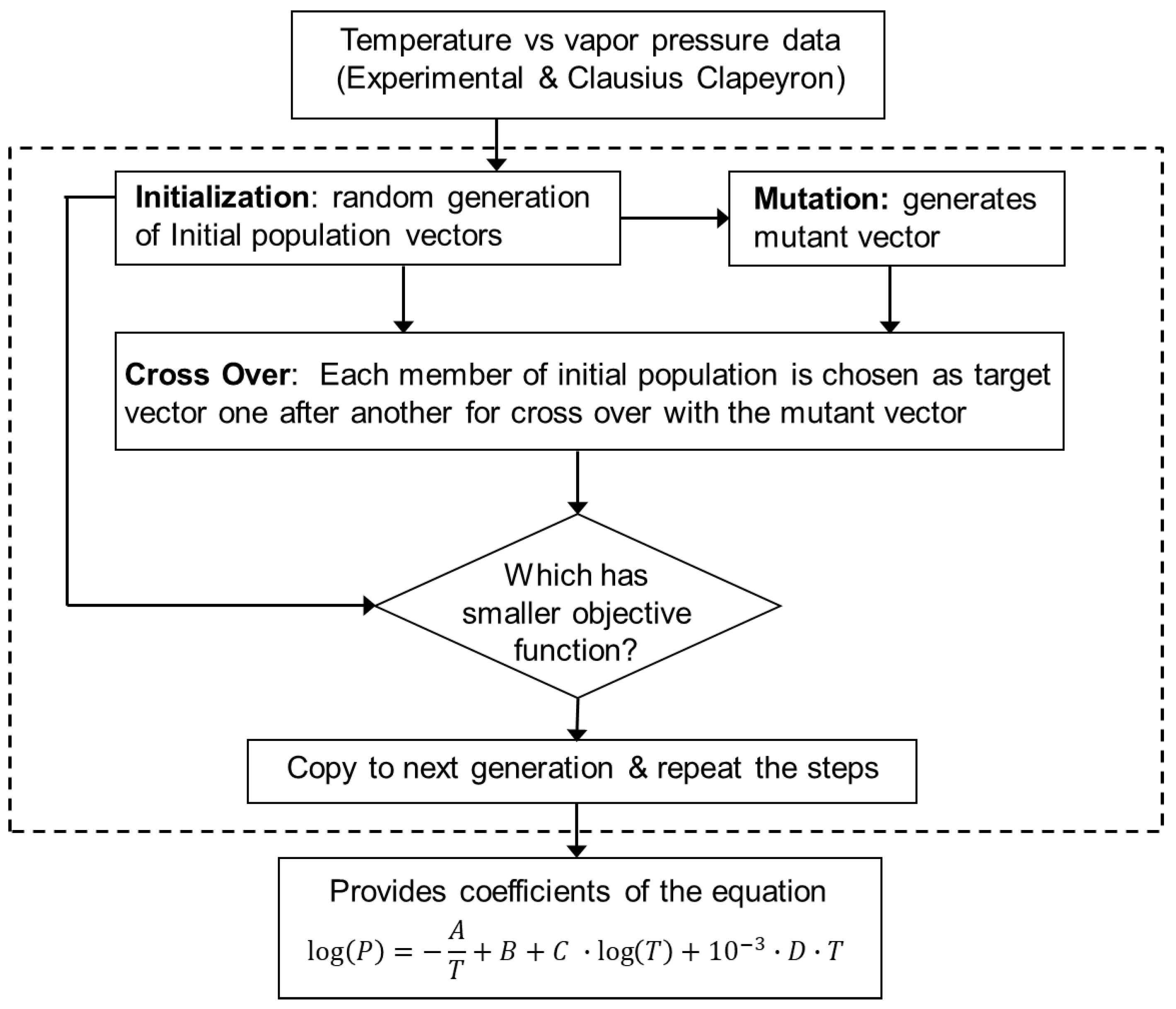
Figure 1. The overall structure of this work. Data collected from experimental work and synthesized using the Clausius Clapeyron equation is fed to a differential evolution genetic algorithm (GA) to provide the coefficients A, B, C, and D of the vapor pressure relation. The dotted box indicates the GA algorithm.
Materials 16 00050 g001
Figure 2. (a) A plot of vapor pressure with temperature for Silicon (Si). The coefficients A = 17,250, B = −15.97, C = 6.403 and D = −0.5281 shown in Table 2 are used in Equation (2) to generate the blue curve in this plot. The region marked by the rectangle is shown separately in 2(b). (b) Enlarged section of the vapor pressure data between 1500 K and 3500 K shows a good fit with the equation. The experimental data from Hultgren et al. [12] and the fitting results between 1700 K and 3400 K are tabulated in the Appendix A.
Materials 16 00050 g002
Figure 3. The variation of vapor pressure with temperature for five commonly used elements of Mg, Al, Ni, Fe, and Ti using the coefficients generated from this study (Table 2) in Equation (2).
Materials 16 00050 g003
Figure 4. (a) A plot of the vapor pressure data of Zn using data from the handbook and the coefficients generated in this study. While Gale et al. [14] provides two different relations denoted by the black squares (between the temperature of 473 K to 692.5 K) and red circles (temperature of 692. K to 1000 K), our work represents the variation in vapor pressure data using a single relation. (b) The enlarged section of the low-temperature vapor pressure data between 400 K and 1000 K shows a good fit with the equation.
Materials 16 00050 g004
Figure 5. A plot showing the decrease in fitness function with the number of generations for Silicon (Si).
Materials 16 00050 g005
Figure 6. (a) A Comparison of the vapor pressure of Li using coefficients generated using our method (GA) and that of Kondo et al. [22]. (b) The enlarged section of the vapor pressure data between 400 K and 1600 K shows the good fit with the equation.
Materials 16 00050 g006
Figure 7. The differences in the vapor pressure data of the recommended relation and that using the previous relation Gale et al. [14] from the experimental data of Hultgren et al. [12] for Pb.
Materials 16 00050 g007
Figure 8. (a) Evaluation of reliability of the proposed equation for calculating vapor pressure. Here, we consider Pb as an example for which data are available between 600 K and 1200 K in works of Alcock et al. [13] and Gale et al. [14] in the range 600 K to 2030 K. (b) A zoomed in version of figure (a) within the temperature range of 600 K to 1200 K and between 0 atm and 1 × 10⁻⁴ atm vapor pressure.
Materials 16 00050 g008
Table 1. Boiling points and enthalpy of vaporization of elements used in the Clausius Clapeyron equation [20,21].
ElementBoiling Point (K)Enthalpy of Vaporization (kJ/mol)
Ag2483254
Al2743284
Au3243342
B4203508
Bi1833179
Ca1760153
Cd1038100
Ce3743398
Co3173390
Cr2945347
Cs963.266.1
Cu2868305
Fe3134354
Ga2673256
Ge3103330
Hf4876648
In2273225
K104779.1
La3743400
Li1603136
Lu3603414
Mg1383132
Mn2373225
Mo4885617
Na116397.4
Nb5017694
Nd3303289
Ni3003379
Os5273678
Pb2017177
Pd3233380
Pt4100510
Rb961.269
Re5903707
Rh4000531
Sc3003310
Se95895.5
Si3533383
Sm2173192
Sn2893290
Sr1653141
Ta5693753
Te1263114
Ti3533427
Tl1733162
V3680444
W6203774
Y3203390
Zn1180115
Zr4650591
Note: The data for Fe were taken from reference 21, while for rest all elements data were taken from ref. [20].
Table 2. Recommended coefficients for the vapor pressure of elements expressed by l o g P = A T + B + C   l o g T + 10 3 D T where P is pressure in atm and T is the temperature in K.
ElementABCDTemperature Range (K)RMSE
Ag21,33065.78−18.161.81100 to 30500.051
Al12,210−27.0610.09−1.161200 to 33700.062
Au29,92085.62−23.531.9131400 to 39750.100
B31,71022.78−4.390.16082000 to 50000.001
Bi10,43010.7−1.5820.079800 to 22800.060
Ca11,61034.36−9.1371.076700 to 22550.024
Cd699428.33−7.6991.57420 to13000.016
Ce22,3909.125−0.869−0.0101600 to 45750.039
Co25,54035.6−8.4610.6521500 to 37500.043
Cr21,79015.86−2.420−0.0241400 to 35250.010
Cs439315.66−3.9730.782400 to 13400.032
Cu21,65046.72−12.261.1241200 to 35000.105
Fe27,18050.1−12.620.85861400 to 37750.003
Ga25,04096.49−27.482.6371050 to 33500.330
Ge82,050386.3−110.78.5991500 to 37500.370
Hf45,98084.44−22.191.4022200 to 56750.093
In6714−44.2415.23−1.7261000 to 27900.365
K494112.69−2.790.436400 to 14100.021
La21,4702.4731.067−0.1471600 to 45750.010
Li6416−17.587.536−1.604700 to 20750.087
Lu29,33058.79−15.471.2141600 to 43250.054
Mg12,04067.15−20.143.482600 to 17300.035
Mn23,60085.49−23.922.1911000 to 30000.118
Mo40,26043.96−10.430.5652200 to 57600.022
Na576411.19 −2.1520.316500 to15100.023
Nb45,52048.26−11.410.6062400 to 58000.051
Nd18,88025.2−5.9370.4271290 to 42250.074
Ni−4552−165.951.135−4.4761500 to 35250.055
Os34,690−21.138.276−0.5872600 to 62000.092
Pb99857.673−0.8340.016800 to 26000.009
Pd25,80055.09−14.6551.3371400 to 38750.028
Pt31,66024.88−5.0160.2351900 to 48500.001
Rb3735−2.6932.567−1.123400 to13250.035
Re50,30052.63−12.510.5212800 to 70250.052
Rh26,6702.4011.319−0.1192000 to 47200.199
Sc16,750−12.215.808−0.8021400 to 37000.121
Se653224.87−6.4641.272500 to 11900.003
Si17,250−15.976.403−0.52811700 to 43000.064
Sm19,14091.49−26.83.113800 to 28000.289
Sn15,9007.795−0.6740.0121200 to 36000.014
Sr965423.6−5.8830.711830 to 21250.010
Ta47,32034.75−7.5340.3262800 to 66500.066
Te12,44073.85−22.013.371600 to 16250.349
Ti26,91028.53−6.3050.4131600 to 41900.080
Tl8591−0.381.895−0.461700 to 22000.012
V37,24073.27−18.971.2211800 to 43750.160
W83,040151.1−38.851.5513000 to73250.262
Y−18,360−246.374.075−5.9681500 to 38000.171
Zn868136.95−10.361.888500 to14750.020
Zr28,580−0.6511.95−0.0762200 to 54750.031
Disclaimer/Publisher’s Note: The statements, opinions and data contained in all publications are solely those of the individual author(s) and contributor(s) and not of MDPI and/or the editor(s). MDPI and/or the editor(s) disclaim responsibility for any injury to people or property resulting from any ideas, methods, instructions or products referred to in the content.