Abstract
Among composites, we can distinguish periodic structures, biperiodic structures, and structures with a functional gradation of material properties made of two or more materials. The selection of the composite’s constituent materials and the way they are distributed affects the weight of the composite, its strength, and other properties, as well as the way it conducts heat. This work is about studying the temperature distribution in composites, depending on the type of component material and its location. For this purpose, the Tolerance Averaging Technique and the Finite Difference Method were used. Differential equations describing heat conduction phenomena were obtained using the Tolerance Averaging Technique, while the Finite Difference Method was used to solve them. In terms of results, temperature distribution plots were produced showing the effect of the structure of the composite on the heat transfer properties.
1. Introduction
Composite materials are materials with specific designed properties. These properties can be obtained by combining certain materials in the relevant way. Composite structures can be characterized by better strength, resistance, or thermal conductivity than their individual component materials. In periodic and biperiodic structures or in those with a functional gradation of properties, it is possible to separate mentally repeatable cells with the same structure. The dimension of such a cell is called the microstructure parameter. Methods that are commonly used in such considerations are certainly the Finite Element Method [1,2]; asymptotic homogenization [3]; the variation of homogenization, introducing additional unknowns called microlocal parameters [4,5]; the higher order theory [6,7]; and the boundary element method [8]. Not all of them take into account the microstructure parameter, in contrast to the Tolerance Averaging Technique, which is used in this work [9,10]. This method is used in the analysis of a variety of structures, such as beams [11,12], plates [13] and shells [14,15]. The main reason for utilizing the Tolerance Averaging Technique in this study was the great alignment of its results to the exact solution when it comes to the stationary problem of heat conduction [16].
The Tolerance Averaging Technique makes it possible to average out the discontinuous coefficients in the heat conduction equation, which result from the different properties of the composite’s constituent materials. The resulting averaged equations, describing the heat flow in the composite structures, were solved numerically using the Finite Difference Method, which was implemented by the authors into MAPLE 2019 software. The proposed FDM algorithm is universal in terms of the dimensions of the composite, its structure, and the type of constituent materials, but not in terms of the assumed boundary conditions of thermal loads, because the number of equations of the Finite Difference Method depends on the number of nodes wherein the sought unknown function is not predetermined.
2. Various Composite Structures of Interest
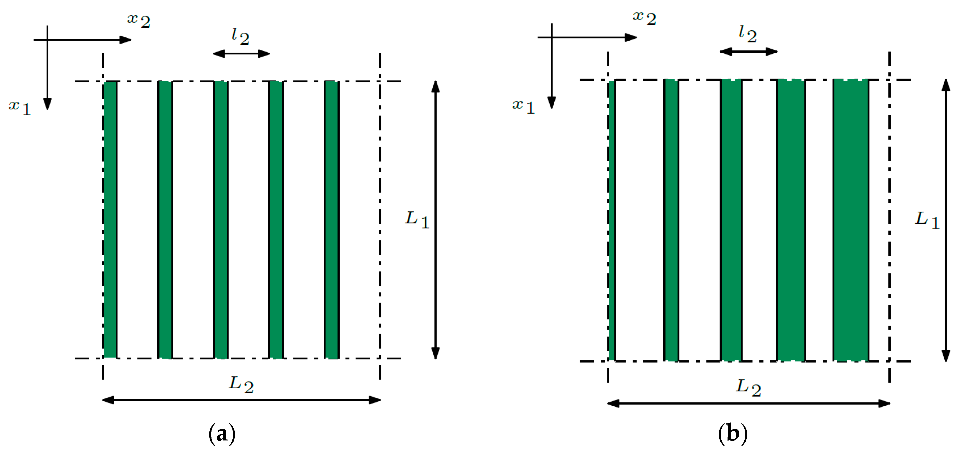
Composite materials are often used in the design of plate and shell structures. Three different structures of this type were analyzed. The first structure is a periodic composite, as shown in Figure 1a. The dimensions of the composite are denoted by L1 and L2 and the material properties change recurrently along the x2-direction.
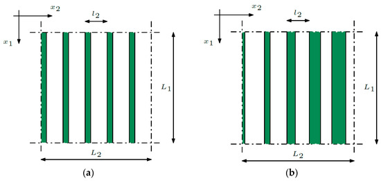
Figure 1.
Composite with (a) periodic structure; (b) functionally graded structure.
The dimension of the mentally separated cell, made of two materials, is denoted by l2. The volume proportion of individual materials in the cell is constant. The volume proportion of the first material is denoted by v1, and the volume share of the second material is denoted by v2, while v1 + v2 = 1.
The second structure is a structure with a functional gradation of properties and is shown in Figure 1b.
The volume proportion of individual materials in the cell is not constant and is determined by a function that depends on the x2-coordinate. Therefore, the volume proportion of the first material is denoted by v1(x2), and the volume share of the second material is denoted by v2(x2).
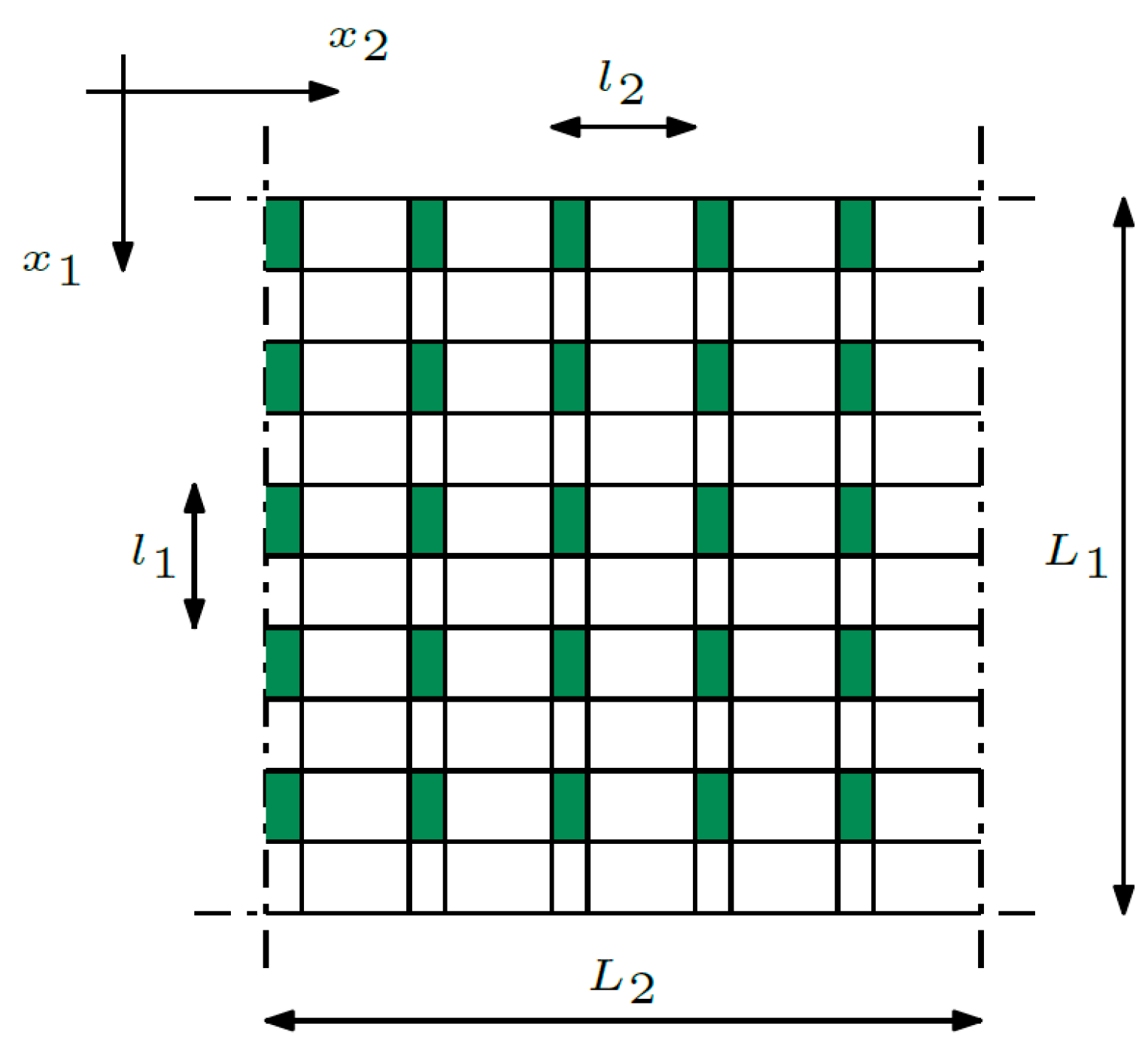
The last one—the third composite—is a biperiodic structure (refer to Figure 2). In the case of this structure, the properties change recurrently along both directions—x1 and x2. The dimensions of the mentally separated cell are denoted by l1 and l2.
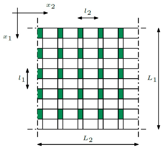
Figure 2.
Biperiodic structure.
The dimension of the cell, called the microstructure parameter, is dependent on the number of composite cells N.
3. Tolerance Averaging Technique
The Tolerance Averaging Technique, mentioned previously, was used to average Equation (1) of the heat transfer issue [17] to replace the terms with discontinuous coefficients:
where θ symbolizes the total temperature field; the components of the tensor of conductivity are denoted by kij (i,j = 1, 2, 3), a specific heat by c and a mass density by ρ. Each cell is composed of two (periodicity) or four (biperiodicity) sub-cells, and the above-mentioned material properties within a given sub-cell are constant.
The technique, used to average the discontinuous coefficients in Equation (1), is constantly developed and used in the analysis of periodic [18,19,20,21,22,23], biperiodic [24,25,26] and functionally graded structures [27,28]. The most relevant assumption of the Tolerance Averaging Technique, from the point of view of the carried-out considerations, is the micro–macro decomposition assumption, according to Equation (2):
where the total temperature field θ is divided into an averaged part ϑ and an oscillating part in the form of product ga·ψa. The average temperature (the so-called macrotemperature) is denoted by ϑ, the fluctuation amplitude of the temperature (the new additional unknowns) is denoted by ψa, and the fluctuation shape functions are denoted by ga. With reference to periodic structures and structures with a functional gradation of properties, index a in (2) is equal to one, and the saw-type function is assumed as the g1-function. The g1-function was chosen based on the available literature and taking into account the specifics of the issue under consideration (the heat conduction issue). This function, shown in Figure 3, provides the continuity of the temperature field and the heat flux between the cells and on interfaces between the first and the second material.
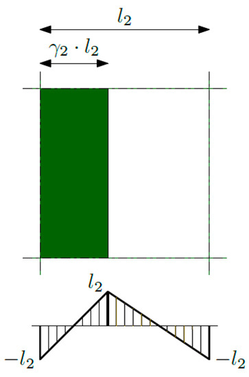
Figure 3.
Fluctuation shape function g1.
With reference to biperiodic structure index, a in (2) runs over 1 and 2. For this structure, which has the fluctuation shape functions g1 and g2, some combination of the saw-type fb and piecewise parabolic hb function was chosen, and it is shown in Figure 4. The fluctuation shape function g1(x1,x2) can be expressed as a product of functions f1(x1) and f2(x2), and the fluctuation shape function g2(x1,x2) can be expressed as a product of functions h1(x1) and h2(x2).
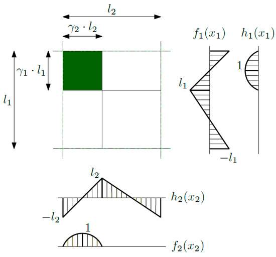
Figure 4.
Fluctuation shape functions g1 and g2.
In addition to the micro–macro decomposition assumption, the Tolerance Averaging Technique also introduces the other assumptions and definitions such as the averaging operation, tolerance-periodic function, slowly varying function (examples include the macro-temperature function ϑ and the fluctuation amplitude ψi) and the highly oscillating function (an example is the fluctuation shape function ga).
By using the above definitions and assumptions of the Tolerance Averaging Technique discussed in [29], the equations with the averaged coefficients describing the heat transfer phenomenon were obtained. The equations in reference to the periodic structure and the structure with a functional gradation of properties (the so-called tolerance model equations) are shown below:
where tensor, whose components are kij, is denoted by K, and is the tensor of conductivity; gradient operator ∇ is expressed as follows (∂1,∂2,∂3); operator ∂ = (∂1,0,0) is a gradient in the x1-direction; and the overlined nabla operator is a gradient in the x2- and x3-directions.
The equations in reference to the biperiodic structure are shown below:
where operator ∂ = (∂1,∂2,0) is a gradient in the x1- and x2-directions and the overlined ∇ operator is a gradient in the x3-direction.
4. Finite Difference Method
It is well-known that the Finite Difference Method, when applied to the differential equation (DE), ordinary equation (ODE) or partial equation (PDE), leads to the system of algebraic linear equations, which is its biggest advantage. The domain of unknown function is narrowed down to a grid of nodes, while the codomain is replaced by set of function values in these nodes. Moreover, every derivative appearing in the DE is approximated by the finite difference quotient, depending very often on function values at adjacent nodes, and that, in particular, may cause a need to temporarily create and use virtual nodes (outside the domain). Function values at virtual nodes are acquired from boundary conditions.
What distinguishes the considered problem from the others is that we actually deal here with the system of PDEs, thus we have more than one unknown function to find. Moreover, each one may have different type of condition in common for all boundaries. Hence, most of the work that has been conducted here was grouping and ordering unknowns and constructing matrix of coefficients for the system. When everything was settled, the MAPLE environment were used in order to implement the Finite Difference Method, and that implementation is further called an algorithm.
To create an algorithm of the Finite Difference Method, it is necessary to divide an analyzed structure into ranges, redefine the tolerance model equations to formulate them in index notation, replace the derivatives appearing in these equations by appropriate differential quotients, and define the boundary conditions, because this affects the number of equations to solve [26]. All of the structures, whether periodic, biperiodic, or with a functional gradation of properties, were discretized along the x1-direction into m ranges, so the number of the nodes along the x1-direction equals m + 1, and analogously along the x2-direction into n ranges, so the number of the nodes along the x2-direction equals n + 1; refer to Figure 5.
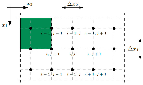
Figure 5.
Discretized composite.
Thus, Δx1 equals L1/m and Δx2 equals L2/n, where L1 and L2 are the dimensions of the composite.
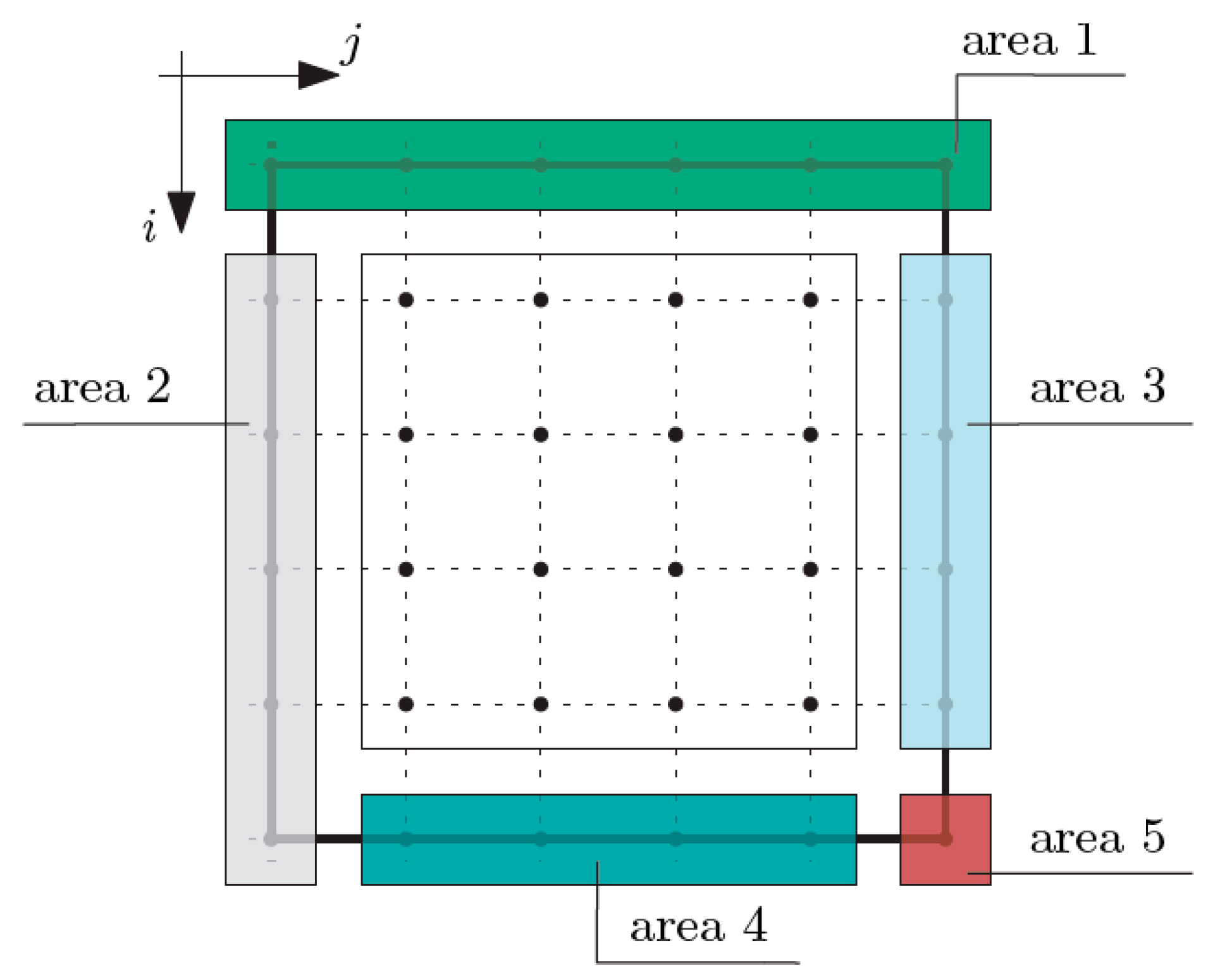
Then, the thermal boundary conditions were formulated, dividing the composite into the areas shown in Figure 6.
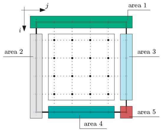
Figure 6.
Areas for the definition of boundary conditions for macro-temperature ϑ.
At the nodes of area 1 (i equals 1 and j is from 1 to n + 1), the total temperature θ is known (defined) and hence the macro-temperature ϑ is also known at these nodes. Analogously, at the nodes of area 2 (i is from 2 to m + 1 and j equals 1), the macro-temperature ϑ is known. The nodes of area 3 (i is from 2 to m and j equals n + 1) and the nodes of area 4 (i equals m + 1 and j is from 2 to n) belong to the right and bottom edges of the composite, which were assumed as thermally insulated, which leads to the following conditions:
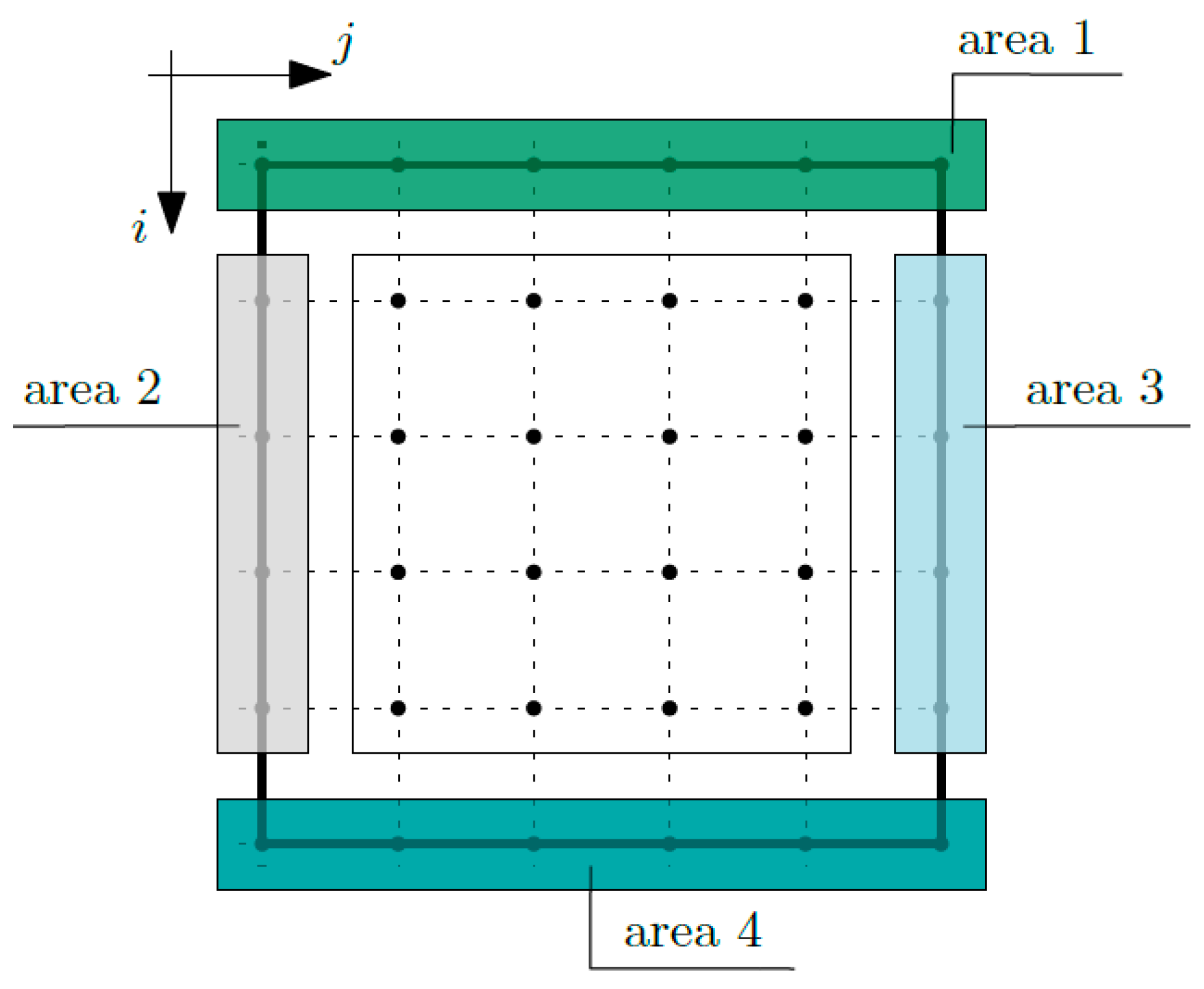
At the nodes of area 5 (i equals m + 1 and j equals n + 1), both conditions expressed by Equations (8)–(9) are defined. Then, the boundary conditions for fluctuation amplitudes of the temperature ψ1 and ψ2 are defined, following the areas shown in Figure 7. At the nodes of area 1 (i equals 1 and j is from 1 to n + 1), the fluctuation amplitudes of the temperature ψ1 and fluctuations amplitudes of the temperature ψ2 are defined. Likewise, the conditions in other areas are: area 2 (i is from 2 to m and j equals 1), area 3 (i is from 2 to m and j equals n + 1) and area 4 (i equals m + 1 and j is from 1 to n + 1).
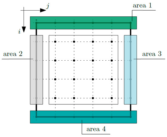
Figure 7.
Areas for the definition of boundary conditions for fluctuation amplitudes ψ1 and ψ2.
After assuming the boundary conditions, the matrix of coefficients appearing in the equations of the tolerance model was defined. These coefficients can be grouped in reference to the equations and individual node areas [25,26]. In an analogous way, the vector of free terms is defined. These terms result from the defined boundary conditions, which are the known values of the macro-temperature ϑ on the top and the left edges of the composite (area 1 and area 2; refer to Figure 6) and the known values of the fluctuation amplitudes of the temperature ψ1 and ψ2 on all of the edges of the composite (areas 1 to 4; refer to Figure 7).
Thus, a system of non-uniform equations was formulated. To solve this system, some variation of the Finite Difference Method was used—the so-called Crank–Nicolson method (the mixed method). The characteristic parameter for this method was assumed to be equal to a half. The Crank–Nicolson method guarantees the convergence of the solution regardless of the division of the structure.
5. Results
Using the created algorithm of the Finite Difference Method [23,25,26,28], calculations were conducted for the three structures described above. The two-dimensional, non-stationary heat-conduction problem of composites with base dimensions equal to L1 = L2 = 1 [m] was analyzed. During the analysis, the composite was assumed to consist of ten cells. In the case of the periodic structure, the dimension of the first sub-cell γ2 is taken initially as equal to 0.25; however, in the case of the structure with a functional gradation of properties, the function of gradation γ2(x2) equals x2/L2. On the other hand, in reference to the biperiodic structure, the volume share of the first sub-cell is originally equal to γ1 · γ2, where γ1 = γ2 = 0.25. The subsequent material properties were preliminarily established for the first sub-cell: c = 500 [J kg−1 K−1], ρ = 7800 [kg m−3], k = 58 [W m−1 K−1] and for the second sub-cell: c = 920 [J kg−1 K−1], ρ = 2720 [kg m−3], k = 200 [W m−1 K−1].
5.1. Periodic and Biperiodic Structure
Firstly, in this section, the approximated results of the Finite Difference Method are presented in the form of 3D-maps of the averaged temperature ϑ and the fluctuation amplitudes ψ1 and ψ2; refer to Figure 8, Figure 9, Figure 10, Figure 11, Figure 12 and Figure 13.
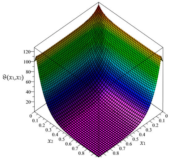
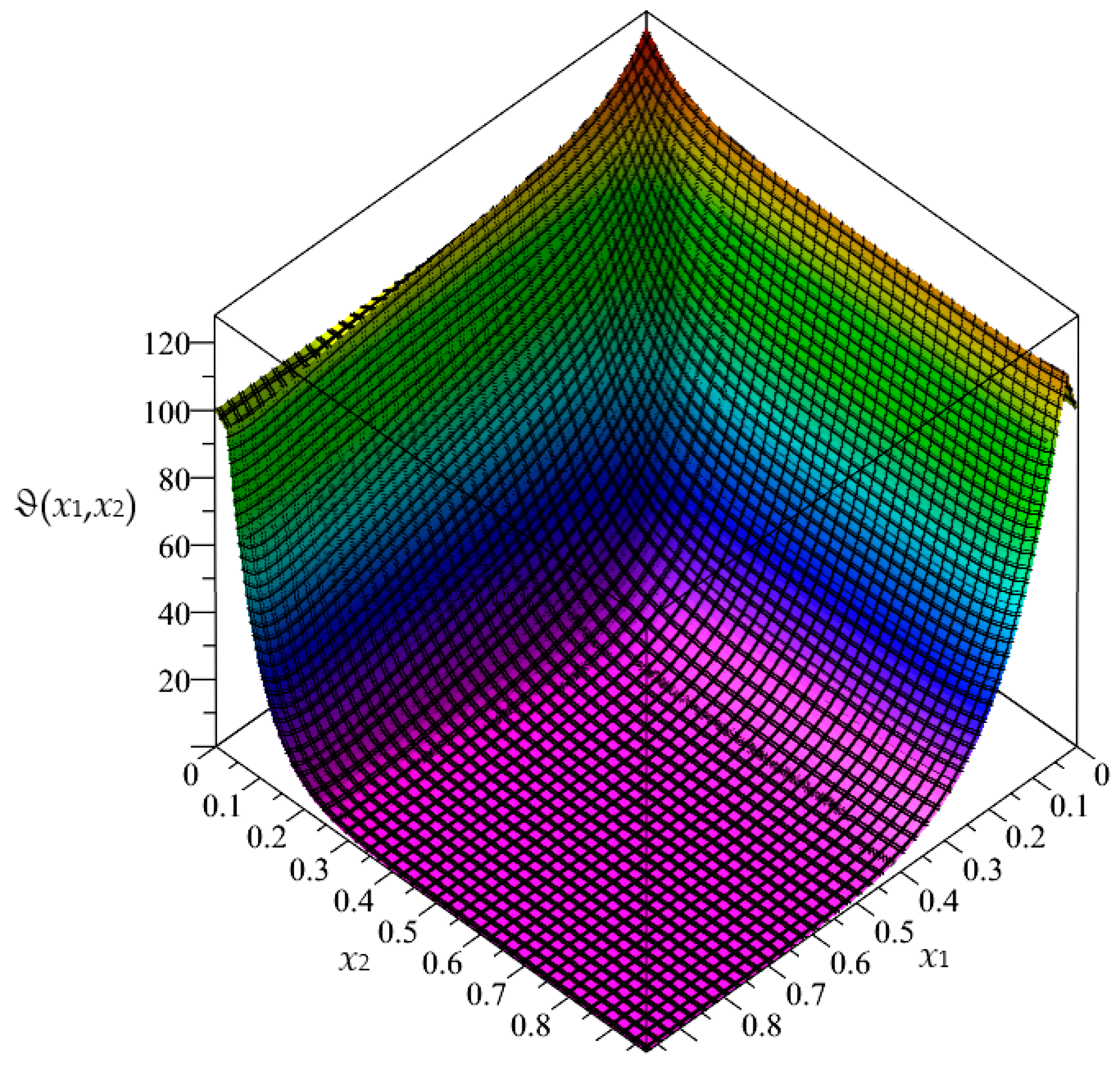
Figure 8.
Map of the averaged temperature ϑ for biperiodic structure.
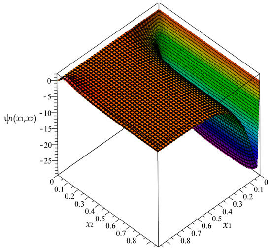
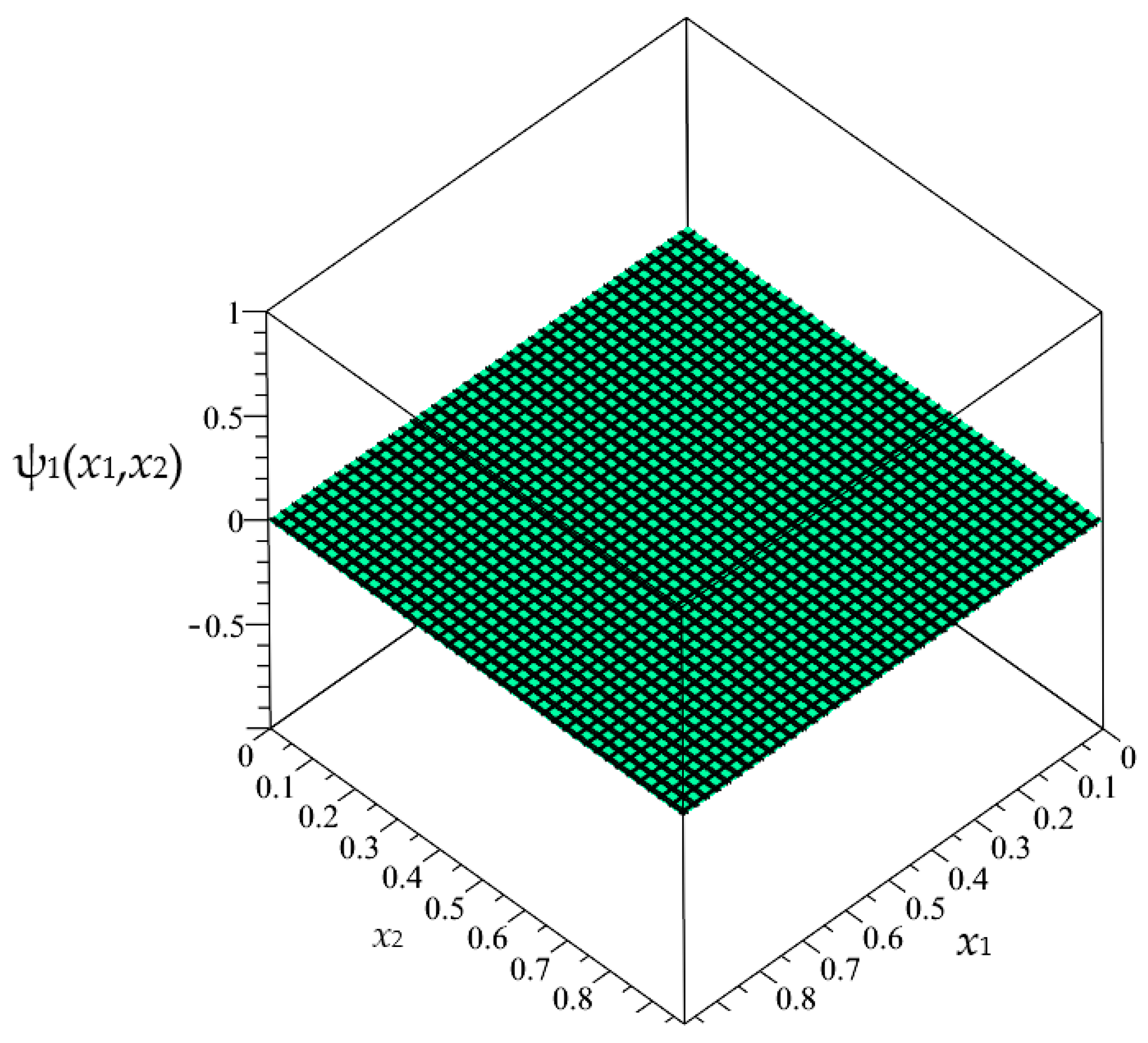
Figure 9.
Map of the fluctuation amplitude ψ1 for biperiodic structure.
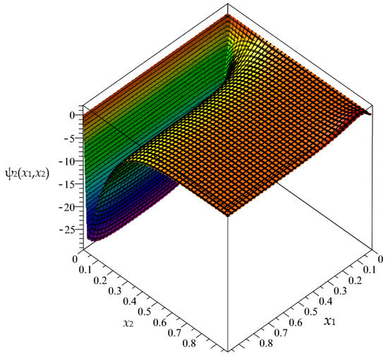
Figure 10.
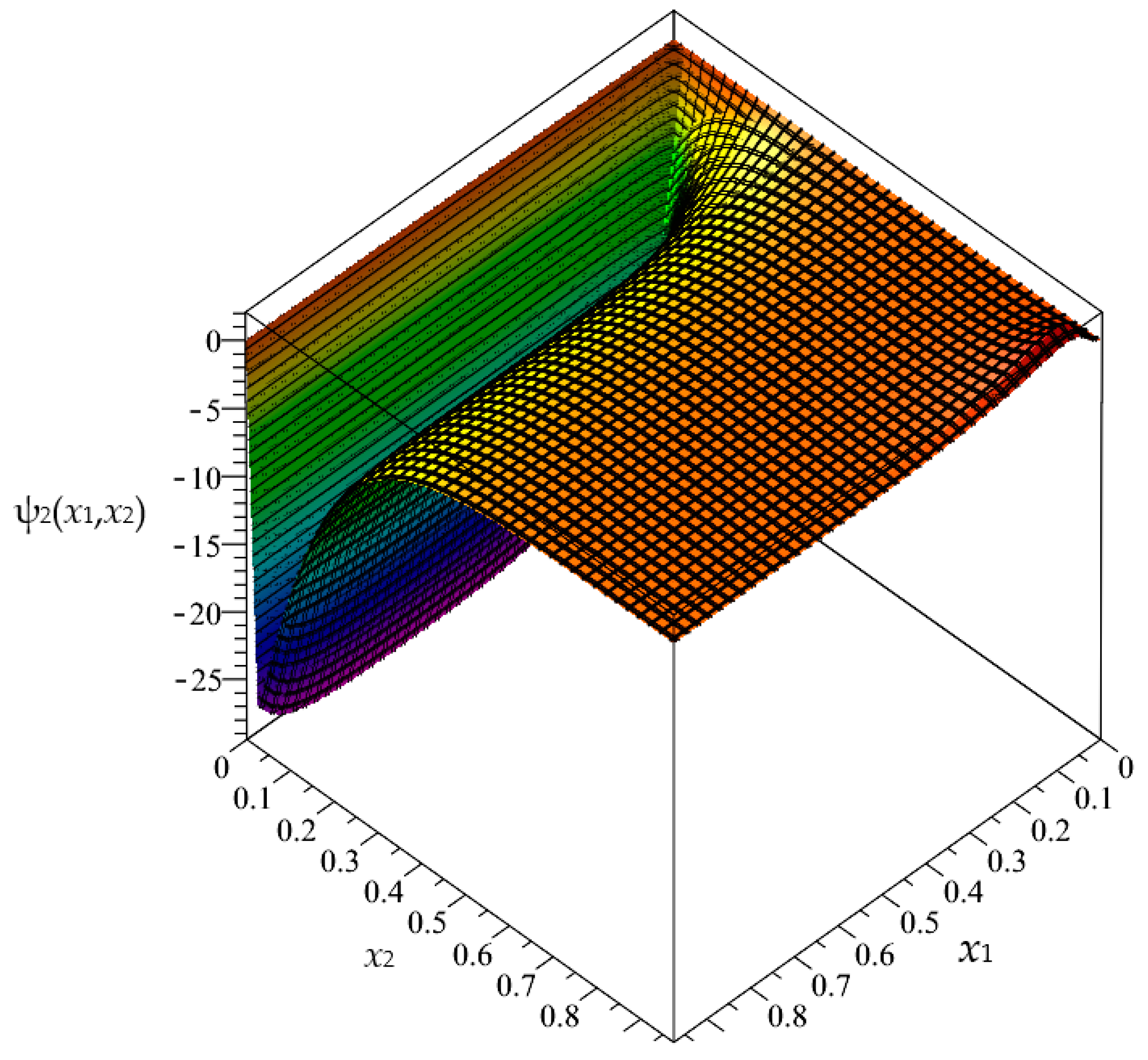
Map of the fluctuation amplitude ψ2 for biperiodic structure.
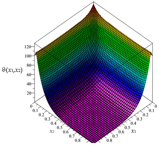
Figure 11.
Map of the averaged temperature ϑ for periodic structure.
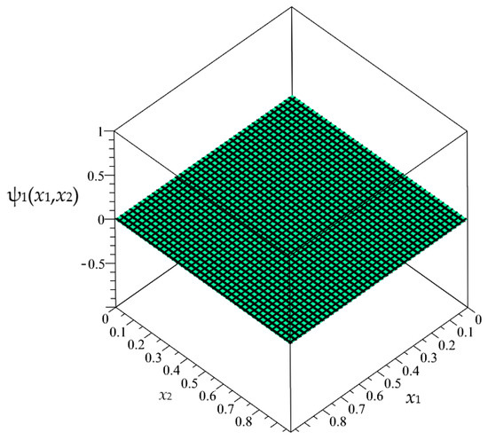
Figure 12.
Map of the fluctuation amplitude ψ1 for periodic structure.
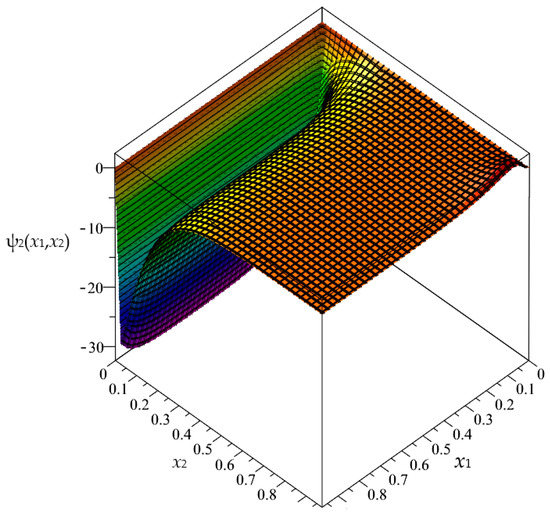
Figure 13.
Map of the fluctuation amplitude ψ2 for periodic structure.
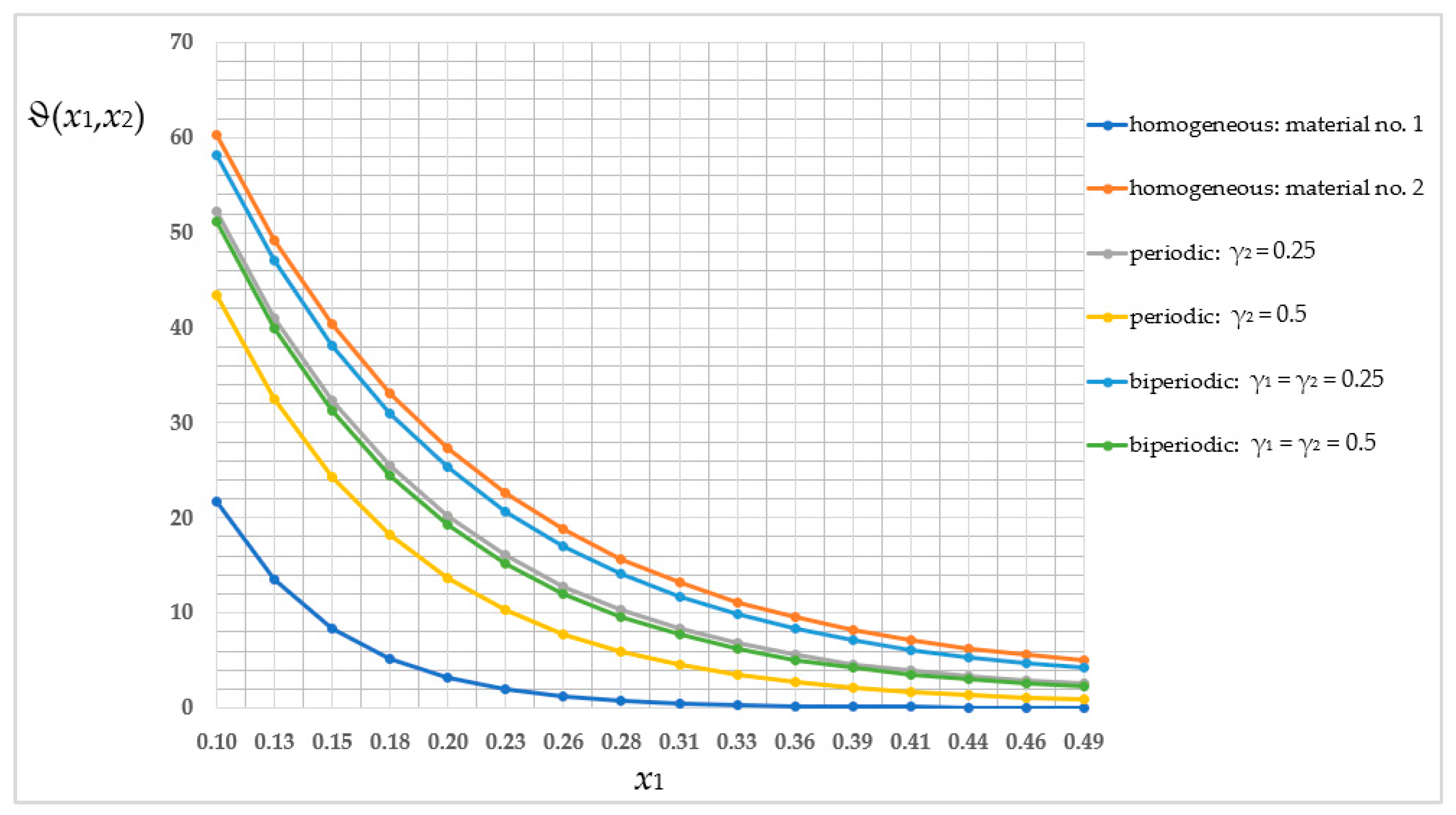
Then, the average temperature distribution was compared in a homogeneous structure with properties of the first sub-cell (blue line), then the second sub-cell (orange line); the periodic structure where γ2 = 0.25 (grey line); the periodic structure where γ2 = 0.5 (yellow line); the biperiodic structure where γ1 = γ2 = 0.25 (light-blue line); and the biperiodic structure where γ1 = γ2 = 0.5 (green line). This comparison of the selected x2-coordinate (x2 = 0.5 [m]) is shown in Figure 14. For the readability of the chart, it is limited to nodes i from 5 to 20.
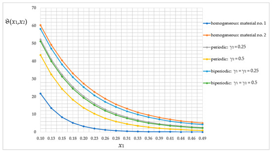
Figure 14.
Comparison of values of the averaged temperature ϑ in selected cross-section.
The values of the averaged temperature, shown in Figure 14, are summarized in Table 1. The lowest temperature values (ignoring the homogeneous structure) were obtained for the periodic structure where γ2 = 0.5, and the highest were obtained for the biperiodic structure where γ1 = γ2 = 0.25. The distinctions in values of the averaged temperature ϑ between these structures are in the order of 25.3–77.1% relative to a higher value.

Table 1.
Values of the averaged temperature [°C].
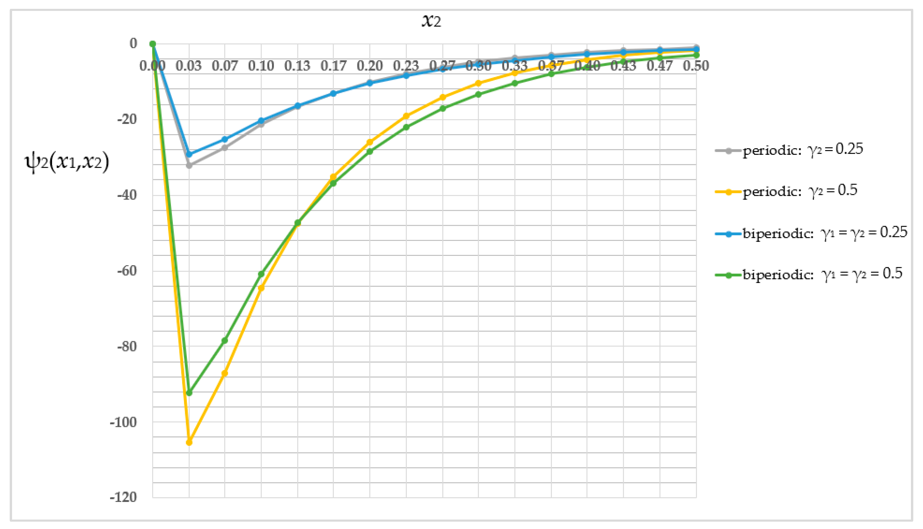
Then, the fluctuation amplitude ψ2 distribution was compared (fluctuation amplitude ψ1 does not occur in the case of the periodic structure) in the periodic structure where γ2 = 0.25 (grey line); the periodic structure where γ2 = 0.5 (yellow line); the biperiodic structure where γ1 = γ2 = 0.25 (light-blue line); the and biperiodic structure where γ1 = γ2 = 0.5 (green line). This comparison for the selected x1-coordinate (x1 = 0.5 [m]) is shown in Figure 15. For the readability of the chart, it is limited to nodes j from 1 to 16.
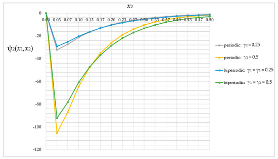
Figure 15.
Comparison of values of the fluctuation amplitude ψ2 in selected cross-section.
The lowest fluctuation amplitude values (the absolute values) were obtained for the biperiodic structure where γ1 = γ2 = 0.25 and the highest were obtained for the periodic structure where γ2 = 0.5. The distinctions in values of the fluctuation amplitude ψ2 between analyzed structures are in the order of 13.65–72.21% relative to a higher value.
5.2. Periodic and Functionally Graded Structure
In this section, the approximated results of the Finite Difference Method are presented in the form of 3D-maps of the averaged temperature ϑ and fluctuation amplitudes ψ1 and ψ2 in reference to the functionally graded structure; refer to confer Figure 16, Figure 17 and Figure 18.

Figure 16.
Map of the averaged temperature ϑ for functionally graded structure.
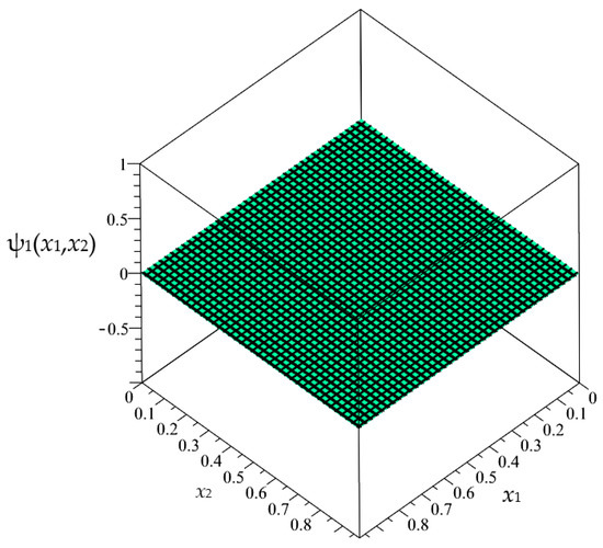
Figure 17.
Map of the fluctuation amplitude ψ1 for functionally graded structure.
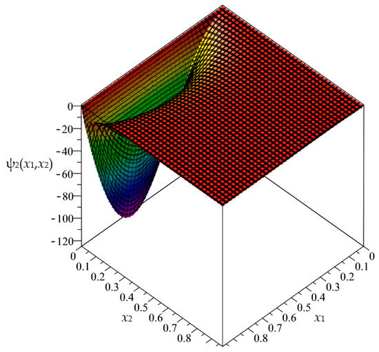
Figure 18.
Map of the fluctuation amplitude ψ2 for functionally graded structure.
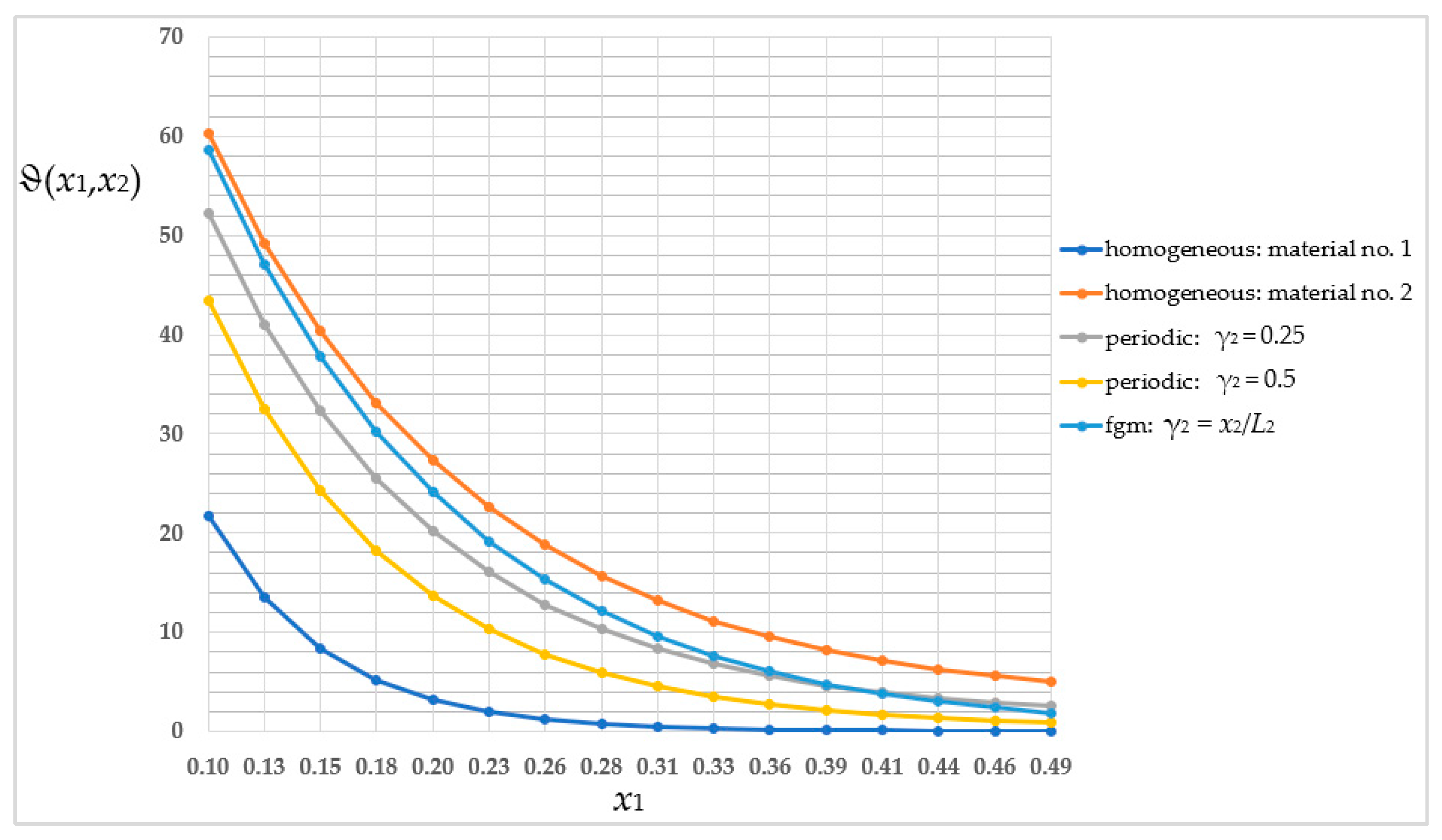
Then, as in the previous section, the averaged temperature distribution was compared in a homogeneous structure with the properties of the first sub-cell (blue line) and of the second sub-cell (orange line); the periodic structure where γ2 = 0.25 (grey line); the periodic structure where γ2 = 0.5 (yellow line); and the structure with a functional gradation of properties where γ2 = x2/L2 (light-blue line). As before, the comparison for the selected x2-coordinate and for nodes i from 5 to 20 is shown in Figure 19.

Figure 19.
Comparison of values of the averaged temperature ϑ in selected cross-section.
The values of the averaged temperature, shown in Figure 19, are summarized in Table 2. For most of the nodes (ignoring the homogeneous structure), the highest values of the averaged temperature were observed for the functionally graded structure. The distinctions in values of the averaged temperature ϑ between the structure with a functional gradation of properties and the periodic structure where γ2 = 0.5 are in the order of 25.91–55.22% relative to a higher value.
Table 2.
Values of the averaged temperature [°C].
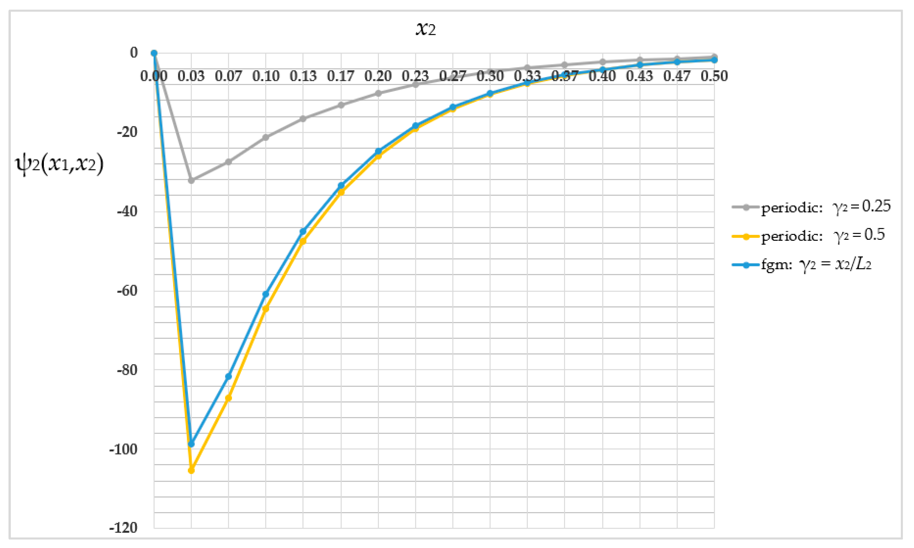
The fluctuation amplitude ψ2 distribution was also compared in the periodic structure where γ2 = 0.25 (grey line); the periodic structure where γ2 = 0.5 (yellow line); and the functionally graded structure where γ2 = x2/L2 (light-blue line). This comparison for the selected x1-coordinate and nodes j from 1 to 16 is shown in Figure 20.
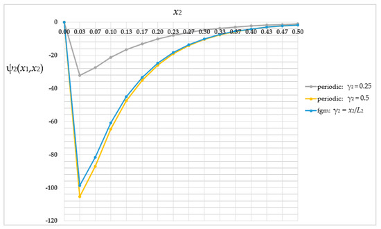
Figure 20.
Comparison of values of the fluctuation amplitude ψ2 in selected cross-section.
The lowest fluctuation amplitude values (the absolute values) were obtained for the periodic structure where γ2 = 0.25 and the highest were obtained for the periodic structure where γ2 = 0.5. The distinctions in values of the fluctuation amplitude ψ2 between analyzed structures are in the order of 34.88–69.41% relative to a higher value.
5.3. Convergence Study
For each of the considered structures, a solution convergence analysis was carried out. The analysis consisted of examining the differences in the values of the unknowns. The solution was assumed to converge when, by increasing the number of intervals Δx1 and Δx2, the differences in the values of the unknowns decreased and were not significant. The results shown in Section 5.1 and Section 5.2, obtained for the number of intervals Δx1 and Δx2, were equal to 40.
5.3.1. Biperiodic Structure
At this point, the results of a solution convergence test for the biperiodic structure are shown. In Table 3, the values of the averaged temperature ϑ(x1,x2) and the fluctuation amplitudes ψ1(x1,x2) and ψ2(x1,x2) for a selected point (x1 = L1/2, x2 = L2/2) and changing number of intervals Δx1 and Δx2 are summarized. In addition, the differences in values of the averaged temperature with the smallest increase in the number of intervals were calculated. These differences were denoted as Δϑ(x1,x2). Analogous differences were calculated for fluctuation amplitudes and denoted as Δψ1(x1,x2) and Δψ2(x1,x2).
Table 3.
Values of the averaged temperature and fluctuation amplitudes for biperiodic structure.
As can be observed in Table 3, the differences in the values of the unknowns decrease as the number of intervals increases. The differences with the smallest increase in the number of intervals are in the order of 0.35–1.02% relative to a higher value.
5.3.2. Periodic Structure
At this point, the results of a solution convergence analysis for the periodic structure are shown. In Table 4, the values of the averaged temperature ϑ(x1,x2) and the fluctuation amplitude ψ2(x1,x2) for a selected point (x1 = L1/2, x2 = L2/2) and changing number of intervals Δx1 and Δx2 are summarized. As in the case of the biperiodic structure, the differences in values of the averaged temperature Δϑ(x1,x2) and the fluctuation amplitude Δψ2(x1,x2) were calculated and analyzed.
Table 4.
Values of the averaged temperature and fluctuation amplitudes for periodic structure.
The differences in the values of the unknowns decrease as the number of intervals increases, and the smallest increase in the number of intervals are in the order of 0.45–1.06% relative to a higher value.
5.3.3. Functionally Graded Structure
For the functionally graded structure, the test of a solution convergence was carried out in the same way as in relation to the previous structures. In Table 5, the values of the averaged temperature ϑ(x1,x2) and the fluctuation amplitude ψ2(x1,x2) for a selected point (x1 = L1/2, x2 = L2/2) and changing number of intervals are summarized. The differences in values of the averaged temperature Δϑ(x1,x2) and the fluctuation amplitude Δψ2(x1,x2) were calculated and analyzed.
Table 5.
Values of the averaged temperature and fluctuation amplitudes for FGM structure.
The differences with a smallest increase in the number of intervals are in the order of 0.41–1.07% relative to a higher value.
6. Conclusions
The main goal of this work was to analyze three types of structures—periodic, biperiodic and those with a functional gradation of properties—under specific thermal boundary conditions. All these studies were possible thanks to a self-created algorithm, the Finite Difference Method, which was implemented into MAPLE software and applied to derived averaged model equations. This work shows the influence of the structure of the composite on the temperature distribution. The dimension of the sub-cell of the composite’s cell is as important as the way and direction of placement of the components; therefore the volume shares of the materials with different properties are also important. As shown in Figure 14 and Figure 19, the values of the averaged temperature ϑ vary significantly, with relative differences in the order of up to 77%. Similarly, as shown in Figure 15 and Figure 20, the values of the fluctuation amplitude ψ2, which impacts in a major way on values of the total temperature field, vary substantially, with relative differences in the order of up to 72%. This leads to the conclusion that by designing the structure of the composite, the expected temperature distribution can be obtained, which in turn is important for the application of this type of construction. The analyzed structures also differ, importantly, in terms of self-weight or stiffness, which can be decisive in choosing the way and direction of the placement of the components and their volume shares.
Author Contributions
Conceptualization, E.K.; methodology, E.K. and P.O.; software, P.O.; validation, P.O.; formal analysis, E.K.; investigation, E.K.; resources, E.K. and P.O.; data curation, E.K.; writing—original draft preparation, E.K.; writing—review and editing, P.O.; visualization, E.K.; supervision, P.O. All authors have read and agreed to the published version of the manuscript.
Funding
This research received no external funding.
Institutional Review Board Statement
Not applicable.
Informed Consent Statement
Not applicable.
Data Availability Statement
Not applicable.
Conflicts of Interest
The authors declare no conflict of interest.
References
- Santos, H.; Mota Soares, C.M.; Mota Soares, C.A.; Reddy, J.N. A semi-analytical finite element model for the analysis of cylindrical shells made of functionally graded materials under thermal shock. Compos. Struct. 2008, 86, 9–21. [Google Scholar] [CrossRef]
- Sadowski, T.; Ataya, S.; Nakonieczny, K. Thermal analysis of layered FGM cylindrical plates subjected to sudden cooling process at one side. Comparison of two applied methods for problem solution. Comput. Mater. Sci. 2009, 45, 624–632. [Google Scholar] [CrossRef]
- Bensoussan, A.; Lions, J.L.; Papanicolay, G. Asymptotic Analysis for Periodic Structures, 1st ed.; North-Holland: Amsterdam, The Netherlands, 1978. [Google Scholar]
- Matysiak, S.J.; Nagórko, W. Microlocal parameters in the modelling of microperiodic plates. Ing. Arch. 1989, 59, 434–444. [Google Scholar] [CrossRef]
- Matysiak, S.J.; Perkowski, D.M. On heat conduction in periodically stratified composites with slant layering to boundaries. Therm. Sci. 2015, 19, 83–94. [Google Scholar] [CrossRef]
- Aboudi, J.; Pindera, M.J.; Arnold, S.M. A coupled higher-order theory for functionally graded composites with martial homogenization. Compos. Eng. 1995, 5, 771–792. [Google Scholar] [CrossRef]
- Aboudi, J.; Pindera, M.J.; Arnold, S.M. Higher-order theory for functionally graded materials. Compos. Part B Eng. 1999, 30, 777–832. [Google Scholar] [CrossRef]
- Sladek, J.; Sladek, V.; Zhang, C.H. Transient heat conduction analysis in functionally graded materials by the meshless local boundary integral equation method. Comput. Mater. Sci. 2003, 28, 494–504. [Google Scholar] [CrossRef]
- Woźniak, C.; Wierzbicki, E. Averaging Techniques in Thermomechanics of Composite Solids. Tolerance Averaging versus Homogenization, 1st ed.; Publishing House of Częstochowa University of Technology: Częstochowa, Poland, 2000. [Google Scholar]
- Jędrysiak, J. Termomechanika Laminatów, płyt i Powłok o Funkcyjnej Gradacji Własności, 1st ed.; Publishing House of Łódź University of Technology: Łódź, Poland, 2010. [Google Scholar]
- Domagalski, Ł. Comparison of the natural vibration frequencies of timoshenko and bernoulli periodic beams. Materials 2021, 14, 7628. [Google Scholar] [CrossRef]
- Jędrysiak, J. Theoretical Tolerance Modelling of Dynamics and Stability for Axially Functionally Graded (AFG) Beams. Materials 2023, 16, 2096. [Google Scholar] [CrossRef]
- Kaźmierczak-Sobińska, M.; Jędrysiak, J. Free Vibrations of Microstructured Functionally Graded Plate Band with Clamped Edges. Vib. Phys. Syst. 2021, 32, 2021216. [Google Scholar]
- Tomczyk, B.; Bagdasaryan, V.; Gołąbczak, M.; Litawska, A. A new combined asymptotic-tolerance model of thermoelasticity problems for thin biperiodic cylindrical shells. Compos. Mater. 2023, 309, 116708. [Google Scholar] [CrossRef]
- Tomczyk, B.; Gołąbczak, M.; Litawska, A.; Gołąbczak, A. Extended tolerance modelling of dynamic problems for thin uniperiodic cylindrical shells. Contin. Mech. Thermodyn. Link Is Disabl. 2023, 35, 183–210. [Google Scholar] [CrossRef]
- Ostrowski, P.; Jędrysiak, J. Dependence of temperature fluctuations on randomized material properties in two-component pe-riodic laminate. Compos. Struct. 2021, 257, 113171. [Google Scholar] [CrossRef]
- Nowacki, W. Elasticity Theory; National Science Publishing House: Warszawa, Poland, 1970. (In Polish) [Google Scholar]
- Domagalski, Ł. Free and forced large amplitude vibrations of periodically inhomogeneous slender beams. Arch. Civ. Mech. Eng. 2018, 18, 1506–1519. [Google Scholar] [CrossRef]
- Marczak, J. The tolerance modelling of vibrations of periodic sandwich structures—Comparison of simple modelling approaches. Eng. Struct. 2021, 234, 111845. [Google Scholar] [CrossRef]
- Tomczyk, B.; Gołąbczak, M. Tolerance and asymptotic modelling of dynamic thermoelasticity problems for thin micro-periodic cylindrical shells. Meccanica 2020, 55, 2391–2411. [Google Scholar] [CrossRef]
- Tomczyk, B.; Bagdasaryan, V.; Gołąbczak, M.; Litawska, A. Stability of thin micro-periodic cylindrical shells; extended tolerance modelling. Compos. Struct. 2020, 253, 112743. [Google Scholar] [CrossRef]
- Jędrysiak, J. Tolerance modelling of vibrations and stability for periodic slender visco-elastic beams on a foundation with damping. Revisiting. Materials 2020, 13, 3939. [Google Scholar] [CrossRef]
- Pazera, E. Heat transfer in periodically laminated structures-third type boundary conditions. Int. J. Comput. Methods 2021, 18, 2041011. [Google Scholar] [CrossRef]
- Tomczyk, B.; Bagdasaryan, V.; Gołąbczak, M.; Litawska, A. On the modelling of stability problems for thin cylindrical shells with two-directional micro-periodic structure. Compos. Struct. 2021, 275, 114495. [Google Scholar] [CrossRef]
- Kubacka, E.; Ostrowski, P. Heat conduction issue in biperiodic composite using Finite Difference Method. Compos. Struct. 2021, 261, 113310. [Google Scholar] [CrossRef]
- Kubacka, E.; Ostrowski, P. A Finite Difference Algorithm Applied to the Averaged Equations of the Heat Conduction Issue in Biperiodic Composites—Robin Boundary Conditions. Materials 2021, 14, 6329. [Google Scholar] [CrossRef] [PubMed]
- Jędrysiak, J.; Kaźmierczak-Sobińska, M. Theoretical analysis of buckling for functionally graded thin plates with microstructure resting on an elastic foundation. Materials 2020, 13, 4031. [Google Scholar] [CrossRef]
- Pazera, E.; Jędrysiak, J. Thermomechanical analysis of functionally graded laminates using tolerance approach. AIP Conf. Proc. 2018, 1922, 140001. [Google Scholar]
- Marczak, J. Tolerance Modelling of Vibrations of a Sandwich Plate with Honeycomb Core. Materials 2022, 15, 7611. [Google Scholar] [CrossRef] [PubMed]


Disclaimer/Publisher’s Note: The statements, opinions and data contained in all publications are solely those of the individual author(s) and contributor(s) and not of MDPI and/or the editor(s). MDPI and/or the editor(s) disclaim responsibility for any injury to people or property resulting from any ideas, methods, instructions or products referred to in the content. |
© 2023 by the authors. Licensee MDPI, Basel, Switzerland. This article is an open access article distributed under the terms and conditions of the Creative Commons Attribution (CC BY) license (https://creativecommons.org/licenses/by/4.0/).