Identification of Differential Drive Robot Dynamic Model Parameters

Abstract

The paper presents the identification process of the mathematical model parameters of a differential-drive two-wheeled mobile robot. The values of the unknown parameters of the dynamics model were determined by carrying out their identification offline with the Levenberg-Marguardt method and identification online with the Recursive least-squares method. The authors compared the parameters identified by offline and online methods and proposed to support the recursive least squares method with the results obtained by offline identification. The correctness of the identification process of the robot dynamics model parameters, and the operation of the control system was verified by comparing the desired trajectories and those obtained through simulation studies and laboratory tests. Then an analysis of errors defined as the difference between the values of reference position, orientation and velocity, and those obtained from simulations and laboratory tests was carried out. On itd basis, the quality of regulation in the proposed algorithm was determined.

1. Introduction

By Industry 4.0 standards, internal transportation is becoming one of the most important areas undergoing transformation. Due to the increasingly scarce labor resources and the increasing cost of transporting products in the production process, transportation is considered in the category of losses. Therefore, there is a need to minimize the costs associated with the internal transportation by reducing the distances and times of product movement. One of the solutions to this problem is the introduction of autonomous transport robots that will accurately, quickly, and safely carry out the tasks assigned to them. Automated guided vehicles are mainly used to support material handling operations—in the warehouse, in production and at the intersection of these areas [1]. This can involve a range of tasks, from the timely delivery of parts to the production line to round-the-clock transportation. Full automation of the production process makes it possible to ensure smooth manufacturing of products along the entire process line. Therefore, in line with the idea of Industry 4.0, more and more often, mobile cart units or AGV (Automated Guided Vehicle) robots appear at the end of the production line to transport and manage products. The market for mobile robots is still at an early stage of development.However, for several years there has been an exponential increase in the implementation of transport mobile robots in the industrial sector.This is due to the fact that more and more companies are noticing the possibilities of this type of vehicles to automate internal transport (Figure 1).

When deciding to integrate mobile robots into a production process at a company, it is necessary to define the efficiency of the transport system based on the following assumptions: the number of robots, the number of logistics points, the location of the navigation paths along which they will move and the frequency of changeovers.

The first automatic carts implementing operator-free driving appeared in the 1950s. These were single implementations primarily in the automotive industry. Over time, the advantages of AGV deployments were increasingly recognized and automatic vehicles began to appear in other industries as well, especially in applications related to in-plant logistics. Since then, AGV robot technology has been developing rapidly, as indicated by the fact that there are several types of AGVs [3,4]. The main characteristic of AGV robots is their driving system. One can distinguish:

• three-wheeled systems (two independent driven wheels, one non-driven castor wheel);
• four-wheeled systems:

  –

  two independent driven standard wheels mounted on the front of the robot and two castor wheels mounted on the rear of the robot;

  –

  four independently controlled Swedish wheels;

• six-wheeled systems (two independent driven standard wheels mounted in the center of the robot frame and four castor wheels mounted on the corners of the robot frame).

All vehicles for automatic load handling are regulated by ISO 3691-4:2020 and called automated guided vehicle (AGV) [5]. This standard distinguishes specific names for different types of AGV introduced by manufacturers of these machines. At the beginning, the main division into AGV and AMR (Autonomous Mobile Robots) can be distinguished. AGV technology refers to automated vehicles that move indoors along physically defined paths, requiring the installation of lines or navigation points. This imposes the need to navigate only along a designated path. In case of encountering an obstacle, it requires stopping and waiting for its removal. Changing the path requires changing the navigation line and other markings. An AMR solution involves autonomous vehicles, often called intelligent vehicles, equipped with 2D or 3D scanners, moving based on a self-created map along a self-determined path between destination points, with the ability to avoid obstacles. The use of AMR technology allows for improved production flexibility.The robot itself determines the optimal route for a given task [6]. Changing the tasks or destinations assigned to it is very quick and does not require physical interference in the space in which the robot moves.

This work proposes a control system for the tracking motion of a mobile robot with two differentially controlled drive wheels and two support wheels. The control system was realized using a kinematic and dynamic controller, where the input and output signals are linear and angular velocity. In the presented approach, the problem is the parameters of the mathematical model of the robot dynamics, which are not available to the user. Therefore, their identification is carried out. In this work, the authors performed offline identification using the Levenberg-Marguardt method based on a pre-recorded trajectory, and online identification using the Recursive least-squares (RLS) method while moving along a desired trajectory. To verify the correctness of the identified parameters, simulation studies were carried out in the MATLAB/Simulink environment, followed by laboratory tests using a real robot. During the tests, the effect of random initial parameters in the identification process on the accuracy of trajectory tracking was investigated. The parameters identified by online and offline methods were compared. The novelty of proposed method is the usage of the parameters identified by the Levenberg-Marguardt method as the initial parameters in the online identification. The effect of combination of online and offline methods on the accuracy of tracking the desired trajectory was investigated.

In Section 2, the authors presented related works. Section 3 presents the selected research object for which the control system, kinematic and dynamic model were developed. The Section 4 contains the results of the identification process, the design of the control system, and the results of trajectory tracking considering the identified parameters. In Section 5, the authors summarized the work carried out.

2. Related Works

AGV robots are a good solution for plants that are characterized by low variability of the production process and not very large distances between logistic destinations. In the case of frequent changes in the production process, dynamically changing environment in the plant (e.g., moving workers) [7], disturbances [8,9] and obstacles [10], a safe and flexible control system is required to allow for environmental changes [11,12,13] or reprogramming of the carts for other tasks. Searching for the most appropriate path planning algorithm according to user requirements can be challenging given the large number of examples existing in the literature [14,15,16,17,18,19]. Furthermore, in the case of AGV robots, the precision of the final positioning is crucial for successful loading and unloading of transported goods in typical industrial applications [20]. Designers of robotics systems use advanced tools to assist in the design process of control systems [21,22,23,24,25] to provide the expected functionality of the robot. The working environment has a particular impact on the change in the operating parameters of the robot. Especially when it is difficult [26,27] such as dusty rooms or industrial and sewage pipelines or mines [28].

A way to obtain unknown values of robot model parameters is to identify them. The work [29,30,31,32] presents a methodology for offline identification based on an inverse dynamics model of robots. The offline identification of the dynamics parameters is sufficient only in the case of robots that will not be expanded with additional modules or will not transport loads. In the case of AGV robots transporting loads, their mass and moment of inertia change, which means that the parameters of the model are not constant. When designing the control algorithm, it is necessary to take into account the possibility of changing the model parameters based on their identification using adaptive methods (online identification) [33,34,35,36,37,38]. The most widely used adaptive methods is the Recursive least squares (RLS) method, as presented in papers [39,40]. The example is for trajectory tracking of an autonomous ground vehicle. To estimate the unknown parameters of the system, the authors of [39] proposed a set-membership-based estimator that provides a nonincreasing estimation error. In the proposed predictive controller (MPC) scheme, the authors used the RLS method to improve prediction accuracy by introducing a robustness constraint on the algorithm to parametric and additive uncertainties. The robustness factor is determined offline based on a set of invariant parameters. The size of this set is updated online. The proposed method is a bit computationally complex, so it requires a high-performance on-board computer. Another example of the use of the RLS method is the work [41], whose authors presented a positioning system for a mobile robot using a stereoscopic camera, an IMU, and an Ultra Wideband (UWB) network containing five positioning markers. The system can be extended with additional positioning markers, whose unknown position in the robot’s environment is estimated using the RLS method and Kalman filter. The proposed system works well in general locating the robot in an unknown environment. However it comes with a large positioning error, which unfortunately is not acceptable for transportation tasks. An interesting approach, consistent with the authors of this work, was demonstrated by the authors of papers [41,42,43,44]. They presented the problem of trajectory tracking by a nonholonomic mobile robot without a global positioning system. The main difficulty pointed out in this work is localizing the robot using only its on-board sensors. The authors proposed an adaptive trajectory tracking controller without orientation and velocity measurements. Their method is not based on the estimation of the robot’s position and velocity from the image of an omnidirectional camera mounted on the robot. The paper [43] presents a fusion of an inertial sensor of six degrees of freedom (6-DoF) which comprises the 3-axis of an accelerometer and the 3-axis of a gyroscope, and a vision to determine a low-cost and accurate position for an autonomous mobile robot. For vision, a monocular vision-based object detection algorithm speeded-up robust feature (SURF) and random sample consensus (RANSAC) algorithms were integrated and used to recognize a sample object in several images taken. In contrast to the work of [42], the authors of this work, present a control concept that not use robot-mounted peripheral devices such as laser scanners and cameras. The tracking control concept is based only on odometry data and inertial measurements.

3. Materials and Methods

The considerations presented in this paper include the TURTLEBOT 2 laboratory robot (Figure 2) [45], which is a low-cost training set, used to building and testing wheeled mobile robot control systems. The platform is equipped with a two-wheeled differential drive and basic sensors such as a laser scanner, a 640 × 480 resolution RGB video camera (used for image processing, color, and texture recognition), an IR camera (depth information processing, distance measurement in the range of 0.4–6.5 m), four directional microphones, and an accelerometer. An advantage of using the robot in this task is its open control system based on ROS (Robot Operating System) [46,47,48], which allows quick launch of the platform and integration with sensors [45]. In addition, the drive system of the TURTLEBOT 2 robot is the basis for expansion to the drive systems discussed in the introduction, commonly used in industrial AGVs. Transferring and adapting the control system to another chassis will be extremely fast and simple.

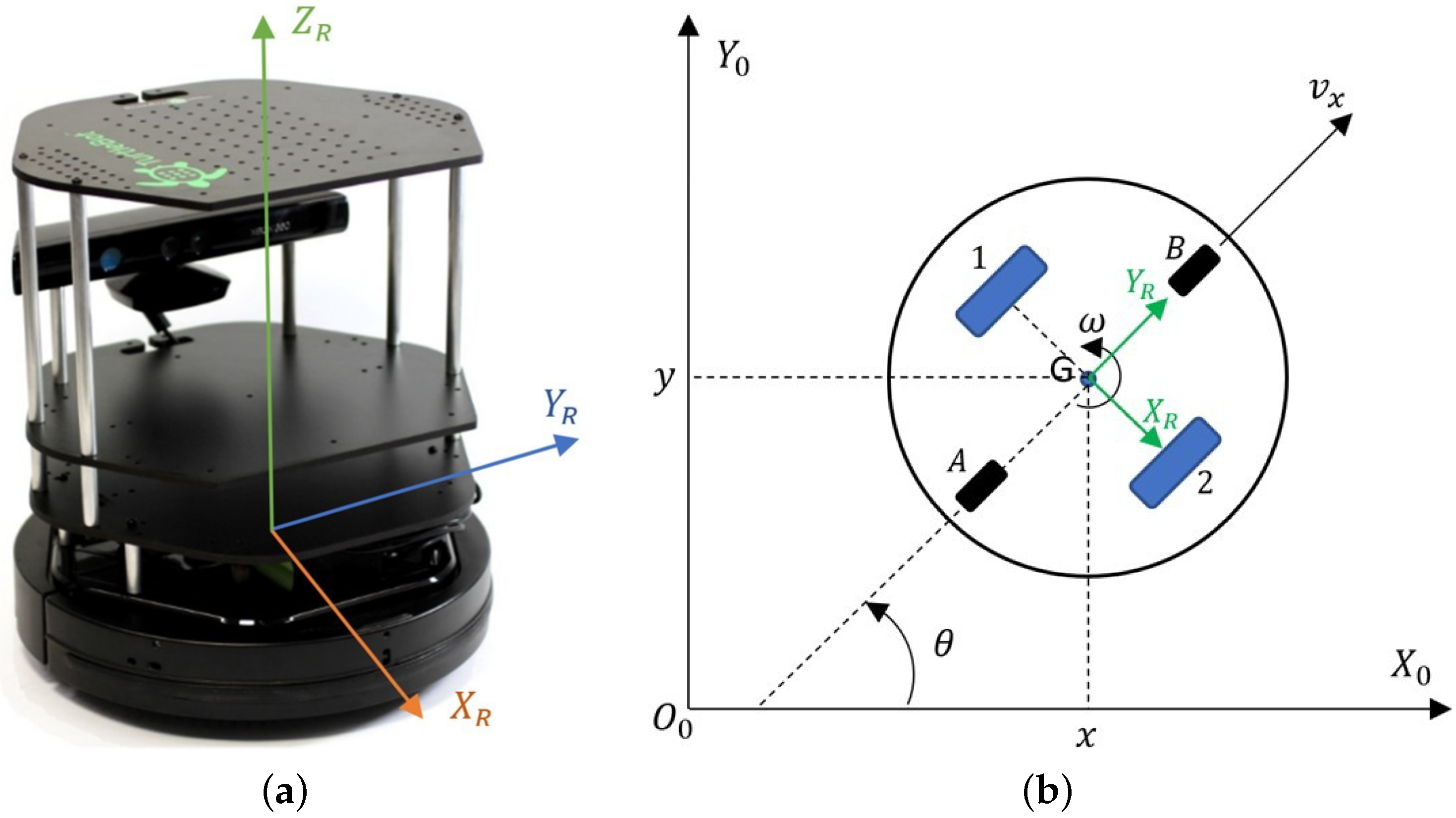
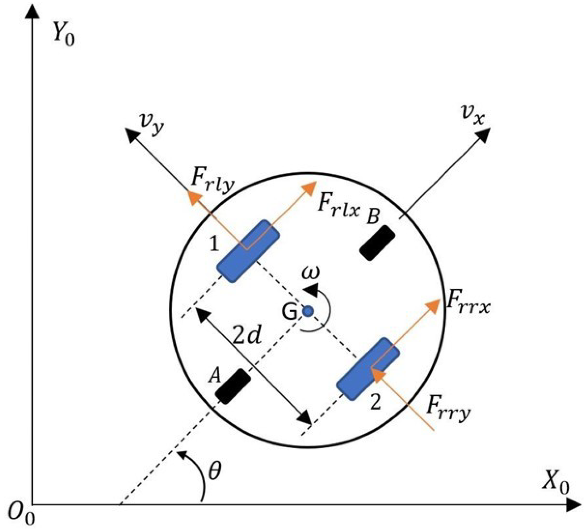
3.1. Kinematic and Dynamic Robot Model

In order to determine the kinematic and dynamic model of the TURTLEBOT 2 robot, the autors used the diagrams shown in Figure 2 and Figure 3.

The $0_0{X}_0{Y}_0$ coordinate system shown in Figure 2b is a global, fixed reference system. The x, y coordinates define the positions and the angle $\theta$ define the orientation of the robot in the global coordinate system. A movable coordinate system $G{X}_R{Y}_R$ with an origin at the geometric center of the robot G, is associated with the base of the robot. The vector $\nu$ determines the linear velocity, while $\omega$ determines the angular velocity of the robot. The numbers 1 and 2 denote the drive wheels, while the letters A and B denote the supporting wheels. The kinematics of the mobile robot TURTLEBOT 2 is described based on [49,50,51,52] by Equation (1) in the form in which the control signals are the linear and angular velocities of the robot:

$$\left[\begin{array}{c}\dot{x}\\ \dot{y}\\ \dot{\theta }\end{array}\right]=\left[\begin{array}{cc}cos\theta & 0\\ sin\theta & 0\\ 0& 1\end{array}\right]\left[\begin{array}{c}v\\ \omega \end{array}\right]$$

(1)

While analyzing the literature in view of control systems, it can be noted that most of the proposed controllers performing the trajectory tracking task consider only the kinematics of the robot. This is an acceptable solution, but in the case of tasks requiring high positioning accuracy and moving at high speed, it is necessary to consider the dynamics of the robot in the control system. In the literature, dynamic models of robots are popular, taking into account torque or motor voltages as steering signals [53,54,55,56]. A much better solution is to use a dynamics model that takes the linear and angular velocities of the robot as control signals [57,58]. This is how commercially available mobile robots are usually controlled. Figure 3 shows a schematic of the TURTLEBOT 2 robot used to determine the dynamics model.

The point G (Figure 3) is not only the robot’s center of mass and center of rotation, but also the tracking point for the desired trajectory. The robot’s velocities are denoted as: ${\nu }_x$—forward velocity, ${\nu }_y$—lateral velocity, $\omega$— angular velocity. In Figure 3, the driving forces of the robot are denoted as $F_{rrx}$, $F_{rry}$—the longitudinal and lateral force of the right wheel and $F_{rlx}$, $F_{rly}$—the longitudinal and lateral force of the left wheel. The dynamics model of the robot was formulated by performing a law of conservation of linear and angular momentum, in the coordinate system associated with the robot, following [59]:

$$\begin{array}{c}\sum F_x=F_{rlx}+F_{rrx}=m\left({\dot{v}}_x-v_y\omega \right)\\ \sum F_y=F_{rly}+F_{rry}=m\left({\dot{v}}_y-v_x\omega \right)\\ \sum M_z=I_z\omega =\frac{d}{2}\left(F_{rrx}-F_{rlx}\right)\end{array}$$

(2)

where:

m—mass of the robot,

$I_z$—moment of inertia of the robot with respect to the axis passing through the point G.

The transformation of the system of Equation (2) (see Appendix A) is the dynamic model of the TURTLEBOT 2 robot as presented:

$$\left[\begin{array}{c}{\dot{v}}_x\\ \dot{\omega }\end{array}\right]=\left[\begin{array}{c}-\frac{{\sigma }_3}{{\sigma }_1}{v}_x\\ -\frac{{\sigma }_4}{{\sigma }_2}\omega \end{array}\right]+\left[\begin{array}{cc}\frac{1}{{\sigma }_1}& 0\\ 0& \frac{1}{{\sigma }_2}\end{array}\right]\left[\begin{array}{c}{v}_{xd}\\ {\omega }_d\end{array}\right]$$

(3)

The model coefficients ${\sigma }_1$…${\sigma }_4$ contain parameters that are very difficult for a laboratory robot user to obtain. These coefficients are functions of the physical parameters of the robot related to drives, gears, internal controls, friction, and are usually not even included in the manuals or technical sheets of the equipment, so their identification was carried out.

3.2. Offline Identification of Robot Dynamic Model Parameters

Before identifying model parameters, it should be checked whether any of the model parameters can be written as a linear combination of two others. In such a case, it would be possible to write the robot dynamics model with the lower number of parameters. Analyzing the developed mathematical model of the robot, the linear independence between the parameters ${\sigma }_1$…${\sigma }_4$ is not clearly visible, because some physical parameters affect more than one parameter ${\sigma }_n$. A detailed analysis is necessary, which was carried out in the work [58] showing that the model parameters ${\sigma }_1$ to ${\sigma }_4$ are independent, that is, they cannot be written as their linear combination. Ultimately, it is necessary to carry out identification of each of the parameters ${\sigma }_1$…${\sigma }_4$.

Offline identification of the parameters of the robot’s dynamics model was carried out using the Levenberg-Marguardt method and measurements of the real test trajectory made by the robot at known constant values of linear and angular velocity. Identification is an iterative process, so in order to perform the first iteration, initial starting values must be entered at the beginning.

To evaluate the impact of starting parameter error on identification time and accuracy, the process was carried out for random initial values of the identified parameter. Starting parameters were described by a normal distribution with expectation value $\mu =1$ variance ${\sigma }^2=1$ in the interval $\langle 0,1\rangle$. The next step was to determine the mean value, the variance and the standard deviation from all samples of the identified parameter.

For the Levenberg-Marguardt method, the minimization criterion takes the form [60,61]:

$${}_d^{min}{\parallel J\left(x\right)d+F\left(x\right)\parallel }_2^2$$

(4)

where $J\left(x\right)$ is the Jacobian of the vector $F\left(x\right)$, and d is the direction of the search for the minimum of the function determined according to the rule:

$$\left[{J\left(x\right)}^{T}J\left(x\right)+\alpha I\right]d=-J\left(x\right)F\left(x\right),for\alpha \ge 0$$

(5)

In the identification process, 50 tests were carried out.

Table 1. Example values of parameters identified by the Levenberg-Marguardt method.

Test No.		${\mathit{\sigma }}_1$	${\mathit{\sigma }}_2$	${\mathit{\sigma }}_3$	${\mathit{\sigma }}_4$	Identification Time [s]
1	Initial values	0.16	0.52	0.96	0.37
	Identified values	4.09	5.46	0.97	0.29	6.65
2	Initial values	0.61	0.26	0.76	0.29
	Identified values	3.14	4.06	0.81	0.24	6.01
3	Initial values	0.59	0.55	0.92	0.29
	Identified values	3.14	4.17	0.83	0.24	6.40
4	Initial values	0.65	0.45	0.55	0.30
	Identified values	3.49	4.63	0.85	0.24	5.92
5	Initial values	0.38	0.56	0.08	0.05
	Identified values	3.37	4.56	0.84	0.26	5.65
	Average	3.47	4.58	0.87	0.25	6.13
	Variance	0.15	0.30	0.00	0.00
	Standard deviation	0.35	0.49	0.06	0.02

contains sample values of the identified parameters of the robot dynamics model.

The low values of the standard deviation of the identified parameters suggest the correctness of the identification process for the Levenberg-Marguardt method, which was verified in simulation and laboratory tests, as presented in Section 4.2, Section 4.3, Section 4.4 and Section 4.5.

3.3. Online Identification of Robot Model Parameters

In a dynamic system, there may be uncertainties in the robot parameters determined by offline methods; therefore, in [40,57,58], adaptation of the robot dynamics model parameters during motion was proposed. In the paper [58], two laws of adaptation of robot dynamics model parameters were presented. The system discussed in this paper uses parameter adaptation based on the expression:

$$\dot{\widehat{\sigma }}={\gamma }^{-1}{A}^T\mathsf{\Delta }-{\gamma }^{-1}\mathsf{\Gamma }\widehat{\sigma }$$

(6)

where $\gamma \in R^{4\times 4}$ is the gain matrix for parameter adaptation, and $\widehat{\sigma }$ is the matrix of estimated parameters of the dynamics model, A is the matrix of velocities and accelerations (see Appendix B), and $\mathsf{\Delta }$ is the matrix of lapses in the form:

$$\mathsf{\Delta }=\left[\begin{array}{c}{v}_{xd}\\ {\omega }_d\end{array}\right]-\left[\begin{array}{c}{v}_x\\ \omega \end{array}\right]$$

(7)

The adaptation law (6) by introducing a gain matrix $\mathsf{\Gamma }\in R^{4\times 4}$ gives the possibility to disable the updating of the model parameters when the error is smaller than a preset limit.

In order to check the effect of unknown model parameters on the initial tracking error of the desired trajectory, two studies were conducted in which random values were used as initial parameters in the identification process. Then the values were replaced with values determined by the offline method.

In the first study, online identification was carried out for random initial parameters described by a normal distribution with expectation value $\mu =1$ and variance ${\sigma }^2=1$ in the interval $\langle 0,1\rangle$. The simulation time was set at 120 s. An example of the distribution of the identified parameters ${\sigma }_1$…${\sigma }_4$ is shown in Figure 4. The values of the starting parameters and those identified by the RLS method are shown in

Table 2. Example values of model parameters identified by the RLS method with random values of initial parameters.

Test No.		${\mathit{\sigma }}_1$	${\mathit{\sigma }}_2$	${\mathit{\sigma }}_3$	${\mathit{\sigma }}_4$
1	Initial values	0.6	0.71	0.22	0.12
	Identified values	3.16	4.15	0.92	0.3
2	Initial values	0.93	0.73	0.49	0.58
	Identified values	3.26	4.51	0.89	0.22
3	Initial values	0.24	0.46	0.96	0.55
	Identified values	3.84	4.34	0.86	0.25
4	Initial values	0.52	0.23	0.49	0.62
	Identified values	3.37	3.87	0.78	0.28
5	Initial values	0.68	0.39	0.37	0.99
	Identified values	3.32	4.16	0.76	0.24
	Average	3.39	4.21	0.84	0.26
	Variance	0.06	0.05	0.00	0.00
	Standard deviation	0.24	0.21	0.06	0.03

.

In the second test of the identification process by the RLS method, the parameters identified by the Levenberg-Marguardt method were used as initial parameters. Figure 5 shows the distribution of the identified parameters ${\sigma }_1$…${\sigma }_4$. The values of the initial and identified parameters by the Levenberg-Marguardt-assisted RLS method are shown in

Table 3. Values of parameters identified by offline-assisted RLS methods.

		${\mathit{\sigma }}_1$	${\mathit{\sigma }}_2$	${\mathit{\sigma }}_3$	${\mathit{\sigma }}_4$
Test No.	Initial values	3.47	4.58	0.87	0.25
1	RLS + offline	3.68	4.49	0.90	0.22
2	RLS + offline	3.66	4.50	0.80	0.22
3	RLS + offline	3.62	4.51	0.85	0.23
4	RLS + offline	3.67	4.52	0.89	0.20
5	RLS + offline	3.62	4.54	0.83	0.24
	Average	3.65	4.51	0.85	0.22
	Variance	0.00	0.00	0.00	0.00
	Standard deviation	0.03	0.02	0.04	0.01

.

4. Results

The correctness of the TURTLEBOT 2 robot’s tracking control algorithm and the correctness of the identification of the parameters of its mathematical dynamic model were checked first by simulation and then by implementation on a real robot. The tests were carried out for an 8-shape trajectory described by a system of equations:

$$\left[\begin{array}{c}{x}_d\\ y_d\\ {\theta }_d\end{array}\right]=\left[\begin{array}{c}{x}_0+A_{x}sin\left({\omega }_{x}t\right)\\ y_0+A_{y}cos\left({\omega }_{y}t\right)\\ atan2\left({\dot{y}}_d,{\dot{x}}_d\right)+k\pi \end{array}\right]$$

(8)

where: $x_0=0$, $y_0=0$, $A_x=2$ [m], $A_y=2$ [m], ${\omega }_x=0.25\left[\frac{\mathrm{rad}}{\mathrm{s}}\right]$, ${\omega }_y=0.125\left[\frac{\mathrm{rad}}{\mathrm{s}}\right]$, $k=0$ if the robot moves forward $k=1$ if the robot moves backwards.

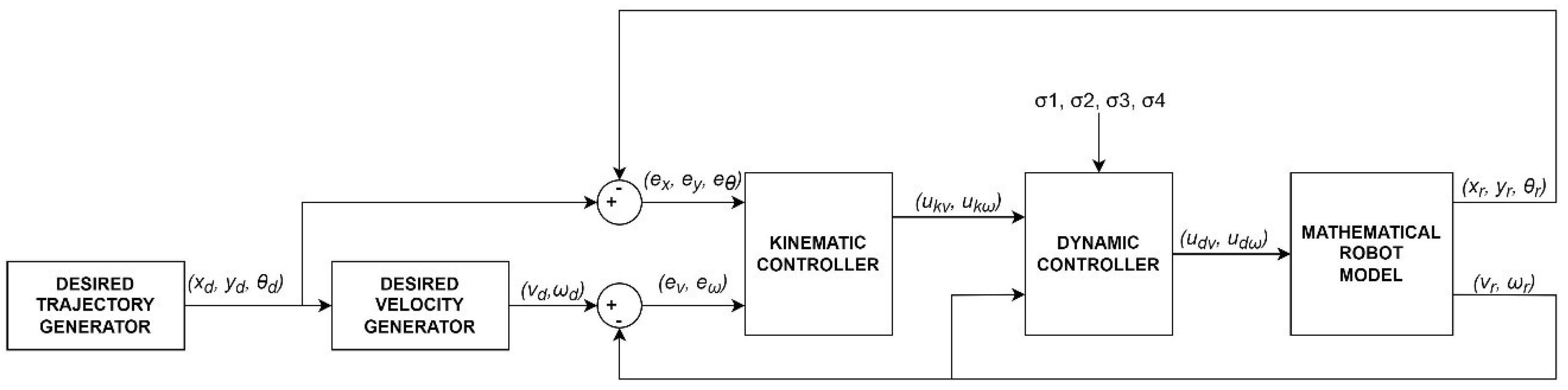
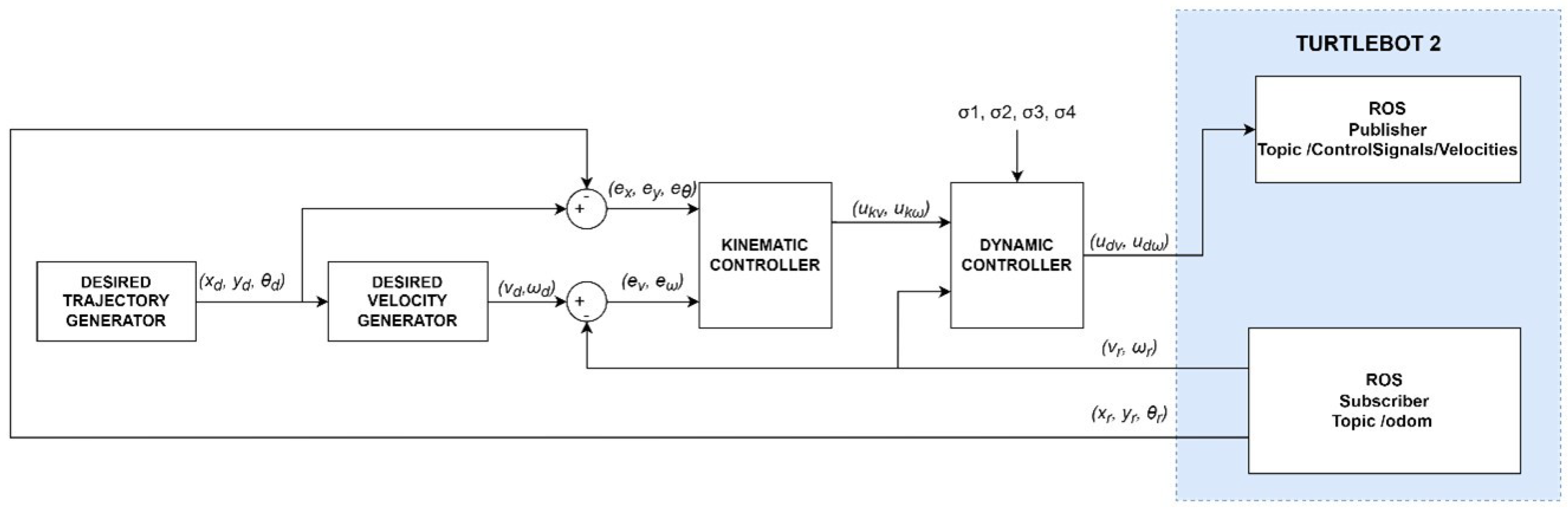
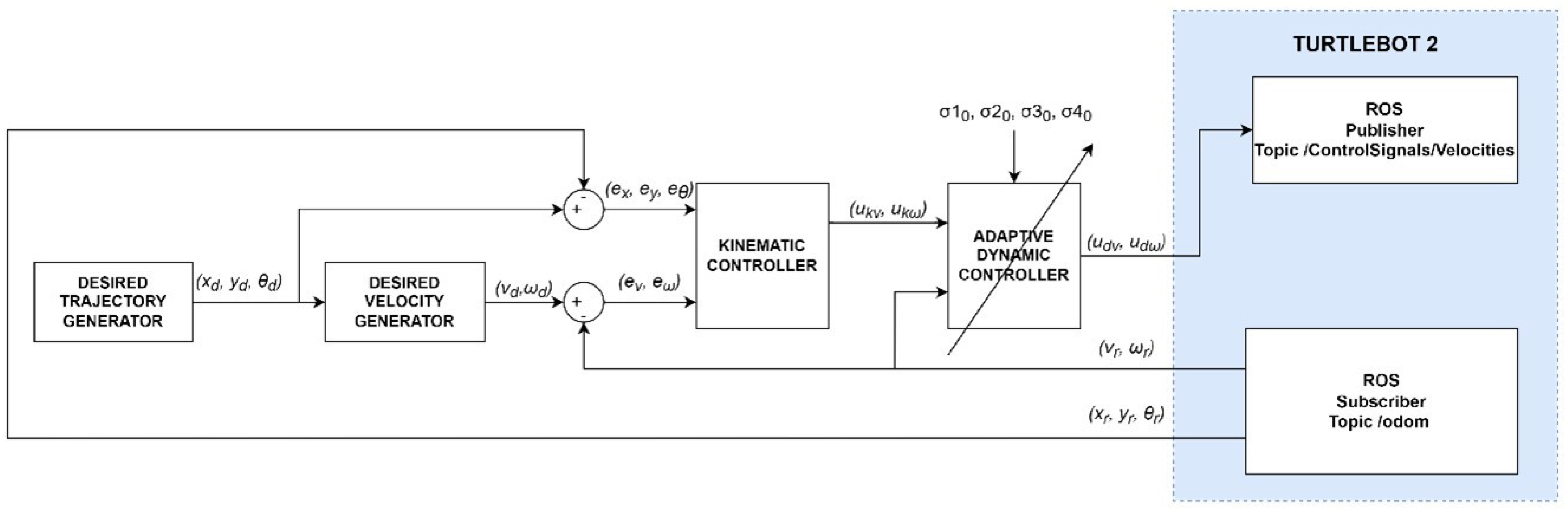
4.1. Kinematic and Dynamic Controller

The implementation of the trajectory tracking task by a robot is always associated with the appearance of errors—the difference between the reference position and the actual position [15,62]. For this purpose, a proportional controller with a feedback loop was proposed, developed based on [63]. Whose task is minimizing the position errors $e_x,e_y,e_{\theta }$ described by Equation (9). It is a transformation of the difference between the desired position and orientation, denoted as $x\left(t\right),y\left(t\right),\theta \left(t\right)$, and the real position and orientation, denoted as $x_r\left(t\right),y_r\left(t\right),{\theta }_r\left(t\right)$:

$$\left[\begin{array}{c}{e}_x\left(t\right)\\ e_y\left(t\right)\\ e_{\theta }\left(t\right)\end{array}\right]=\left[\begin{array}{ccc}cos\theta \left(t\right)& sin\theta \left(t\right)& 0\\ -sin\theta \left(t\right)& cos\theta \left(t\right)& 0\\ 0& 0& 1\end{array}\right]\left[\begin{array}{c}x\left(t\right)-x_r\left(t\right)\\ y\left(t\right)-y_r\left(t\right)\\ \theta \left(t\right)-{\theta }_r\left(t\right)\end{array}\right]$$

(9)

The kinematic controller proposed based on [63] takes the form:

$$\left[\begin{array}{c}{u}_{kv}\left(t\right)\\ u_{k\omega }\left(t\right)\end{array}\right]=\left[\begin{array}{ccc}-k_1& 0& 0\\ 0& -sign\left(v_r\left(t\right)\right)k_2& -k_3\end{array}\right]\left[\begin{array}{c}{e}_x\left(t\right)\\ e_y\left(t\right)\\ e_{\theta }\left(t\right)\end{array}\right]$$

(10)

where ${\nu }_r\left(t\right)$—real linear velocity, $u_{k\nu }\left(t\right)$ and $u_{k\omega }\left(t\right)$ are the control signals of the kinematic controller (linear and angular velocity) and its gains $k_1,k_2,k_3$ are determined from the following equations [63]:

$$\begin{array}{cc}\hfill & k_1=k_3=2\epsilon {\omega }_n\left(t\right),for\epsilon \in \left(0,1\right),b>0\hfill \\ \hfill & k_2=b\ast \left|v_r\left(t\right)\right|\hfill \\ \hfill & {\omega }_n\left(t\right)=\sqrt{{{\omega }_r}^2\left(t\right)+b{v_r}^2\left(t\right)}\hfill \end{array}$$

(11)

where:

$\epsilon$—damping coefficient, ${\omega }_n\left(t\right)$—characteristic frequency, b—additional control coefficient, ${\omega }_r\left(t\right)$—real angular velocity.

The assumption for the development of the dynamic controller was to treat the control signals from the kinematics controller (linear and angular velocity) expressed by relation (10) as reference signals. The control law for the dynamic controller was developed based on the inverse dynamics (Appendix B), using the parametric model of robot dynamics (3) and the considerations presented in the paper [58]. The control law is described by the equation:

$$\begin{array}{cc}\hfill & \left[\begin{array}{c}{u}_{dv}\left(t\right)\\ u_{d\omega }\left(t\right)\end{array}\right]=\left[\begin{array}{cc}{\sigma }_1& 0\\ 0& {\sigma }_2\end{array}\right]\left[\begin{array}{c}{\vartheta }_1\\ {\vartheta }_2\end{array}\right]+\left[\begin{array}{cc}\begin{array}{cc}\begin{array}{c}0\\ 0\end{array}& \begin{array}{c}0\\ 0\end{array}\end{array}& \begin{array}{cc}\begin{array}{c}{v}_r\left(t\right)\\ 0\end{array}& \begin{array}{c}0\\ {\omega }_r\left(t\right)\end{array}\end{array}\end{array}\right]{\left[\begin{array}{cc}\begin{array}{ccc}{\sigma }_1& {\sigma }_2& {\sigma }_3\end{array}& {\sigma }_4\end{array}\right]}^T\hfill \\ \hfill & {\vartheta }_1=\dot{v}\left(t\right)+k_v\left(u_{kv}\left(t\right)-v_r\left(t\right)\right)\hfill \\ \hfill & {\vartheta }_2=\dot{\omega }\left(t\right)+k_{\omega }\left(u_{k\omega }\left(t\right)-{\omega }_r\left(t\right)\right)\hfill \end{array}$$

(12)

where $k_{\nu }$ and $k_{\omega }$ are gains, $u_{dv}\left(t\right)$ and $u_{d\omega }\left(t\right)$ are control signals of the dynamic controller.

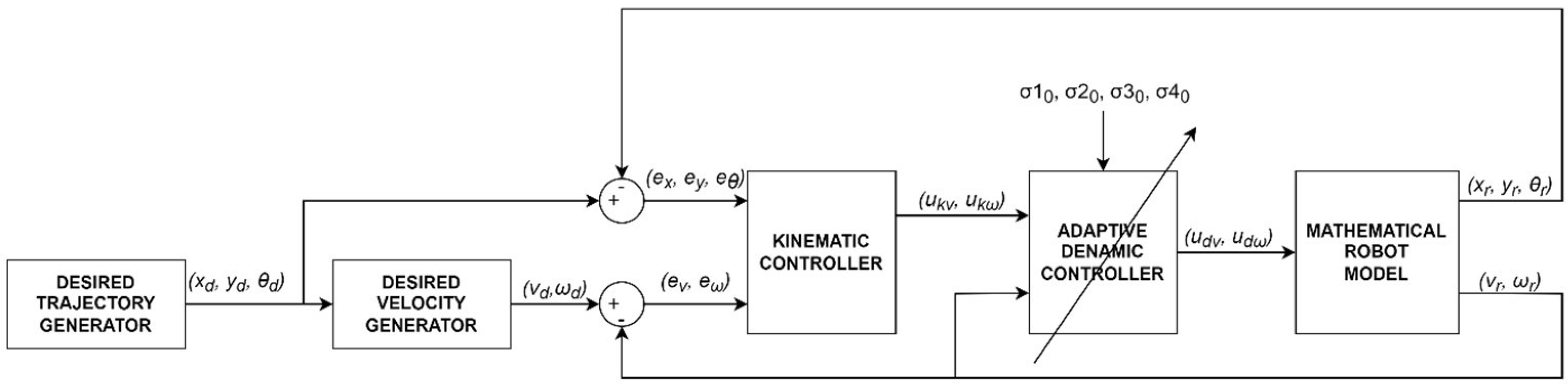
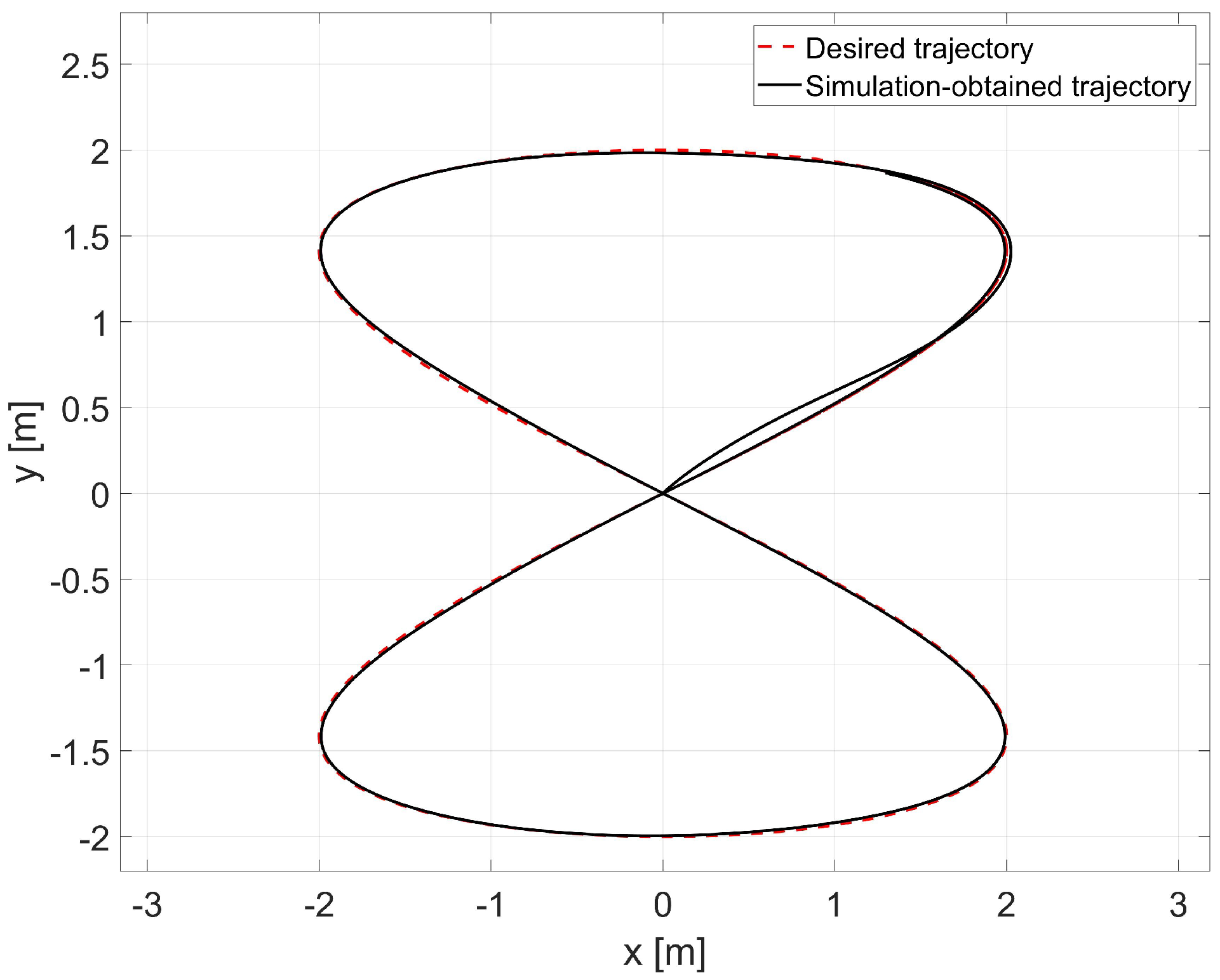
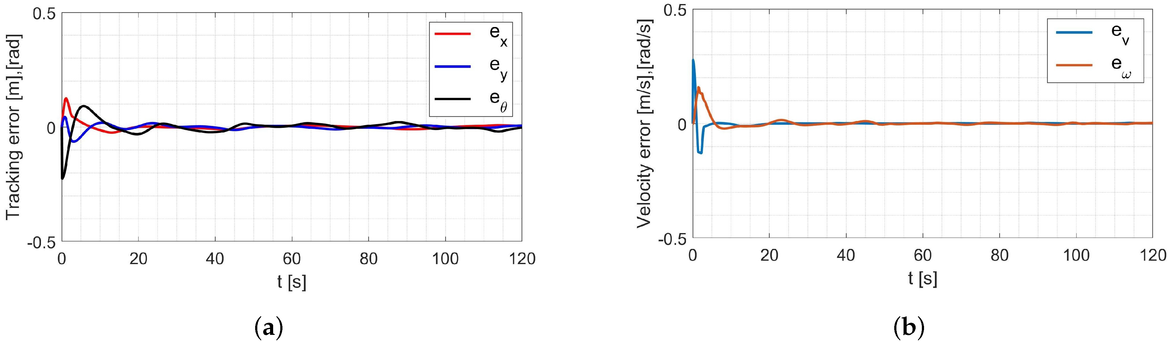
4.2. Simulation Tests of the Control System Considering Parameters Identified Offline

Simulation of the tracking motion of the TURTLEBOT 2 robot (Figure 6) was developed in MATLAB/Simulink environment, using the identified parameters of the robot model. The control system is composed of a:

• desired trajectory generator module that determines the position $x_d$, $y_d$ and orientation ${\theta }_d$,
• a generator of the desired linear velocity $v_d$ and angular velocity ${\omega }_d$,
• a kinematic controller described by Equation (10),
• a dynamic controller described by Equation (12),
• and a mathematical model of the robot described by Equations (1) and (3).

Figure 6. Block diagram of the tracking motion simulation of the TURTLEBOT 2 robot.

Figure 6. Block diagram of the tracking motion simulation of the TURTLEBOT 2 robot.

In the simulation, the average values of the model parameters shown in Table 1 were used. A comparison of the desired trajectory and the simulation-obtained trajectory, using the parameters identified by the Levenberg-Marguardt method is shown in Figure 7. The position and orientation errors are shown in Figure 8a, while the velocity errors are shown in Figure 8b.

Based on the analysis of the simulation-determined errors for the Levenberg-Marguardt method (Figure 8), it can be concluded that the controller, developed based on the inverse dynamics with the parameters identified by the Levenberg-Marguardt method, realizes control in tracking motion with position, orientation and velocity errors no greater than:

• in the x-axis direction: $e_x=0.007\left[\mathrm{m}\right]$,
• in the y-axis direction: $e_y=0.007\left[\mathrm{m}\right]$,
• orientation: $e_{\theta }=0.021\left[\mathrm{rad}\right]$,
• linear velocity $e_v=0.001\left[\frac{\mathrm{m}}{\mathrm{s}}\right]$,
• angular velocity $e_{\omega }=0.007\left[\frac{\mathrm{rad}}{\mathrm{s}}\right]$.

The regulation time for the case of an 8-shape trajectory tracking task is equal to $t_r\approx 8.2\left[\mathrm{s}\right]$.

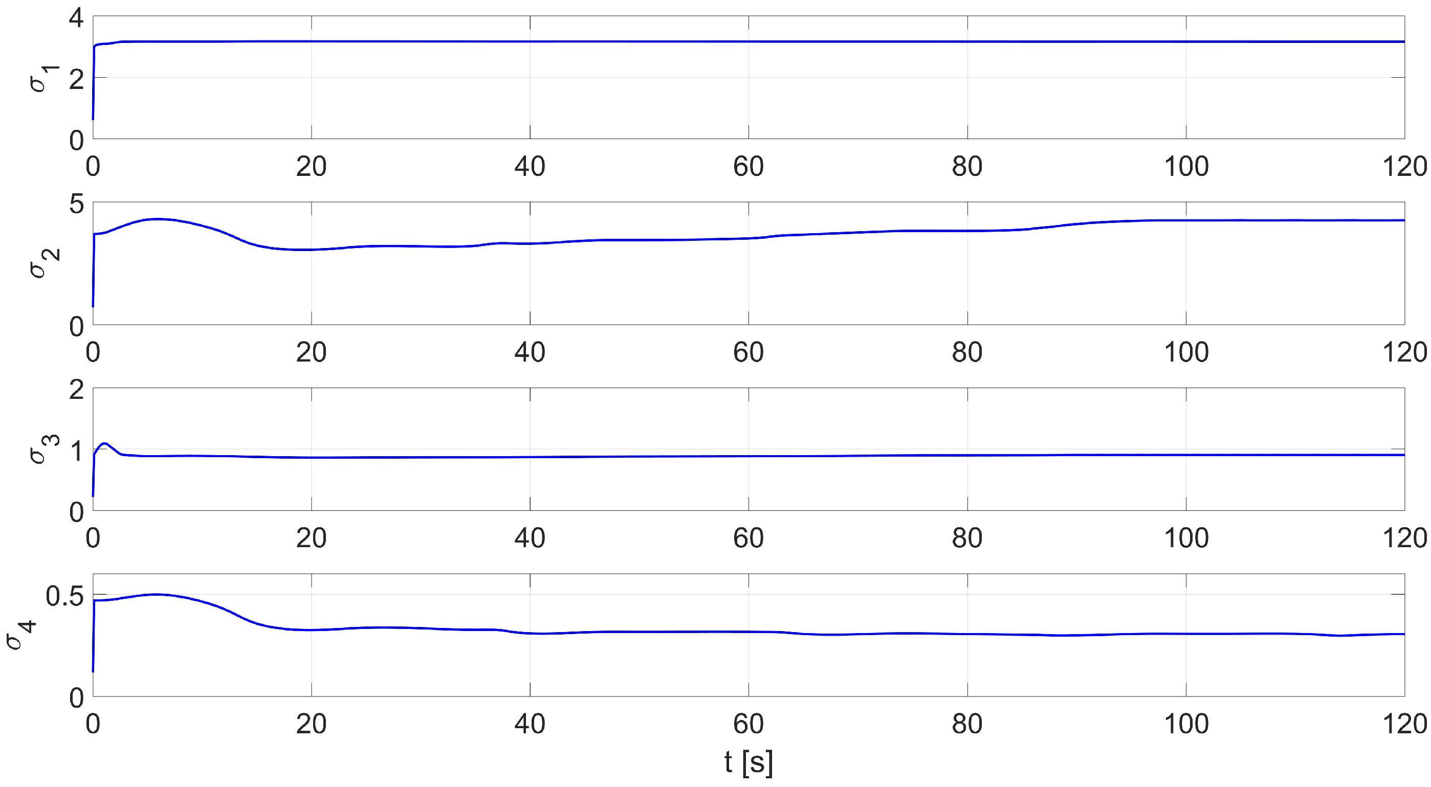
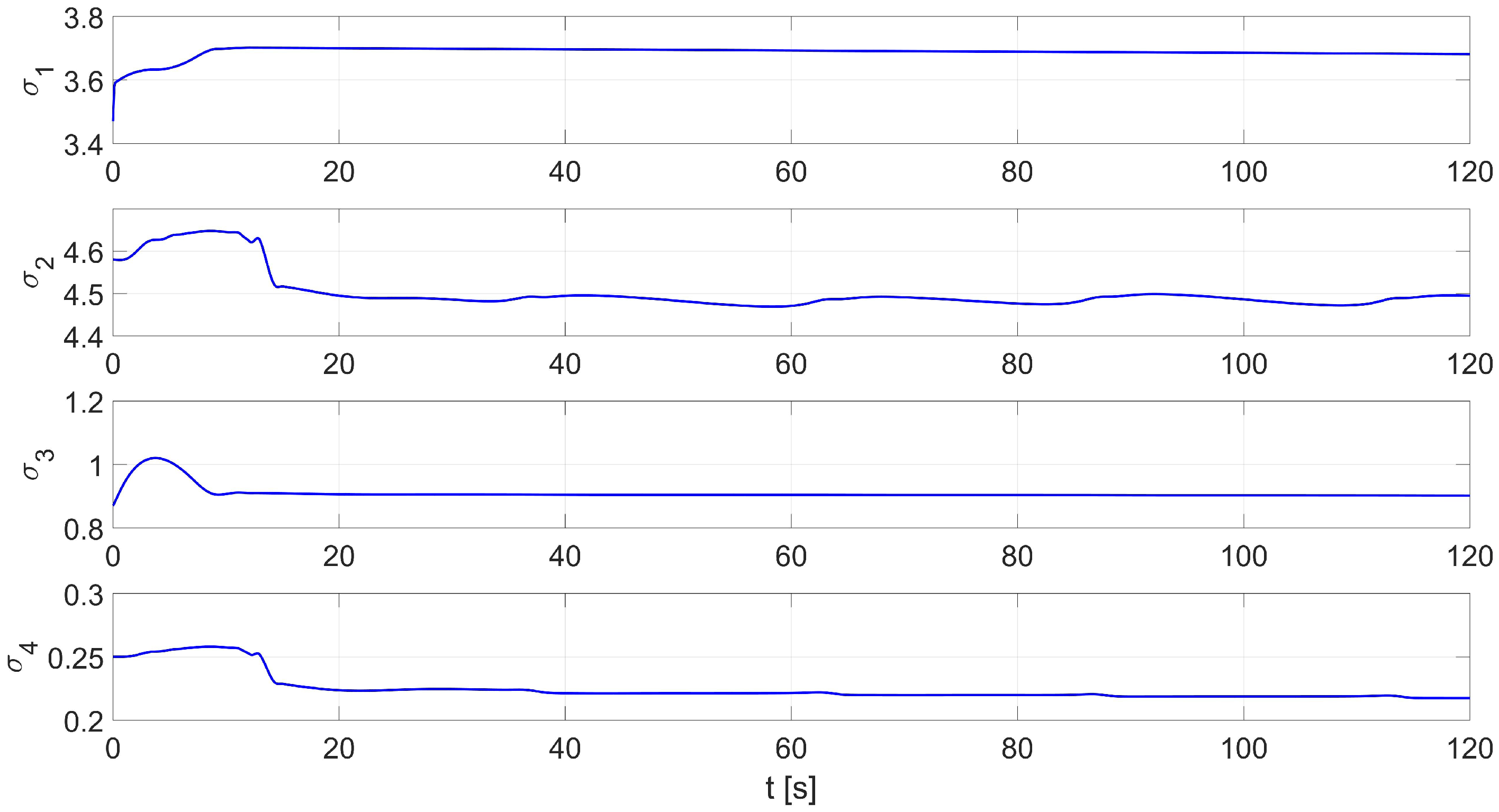
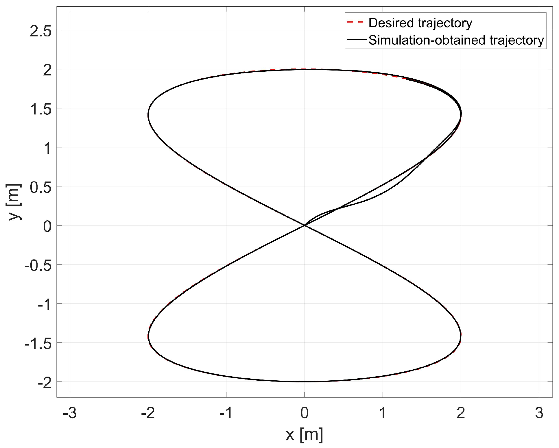
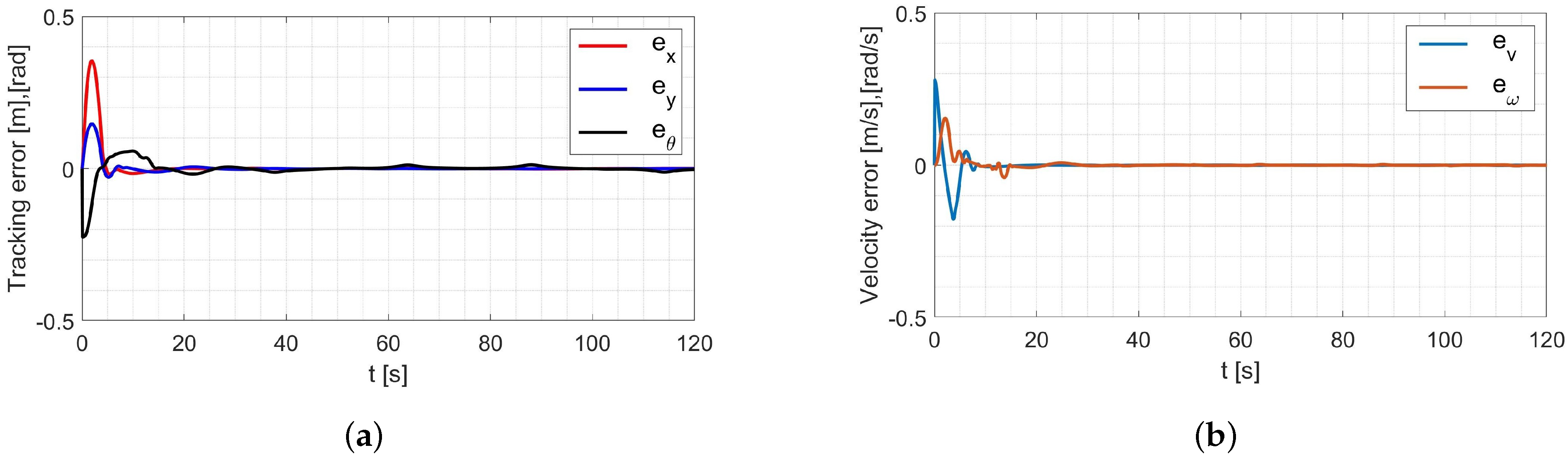
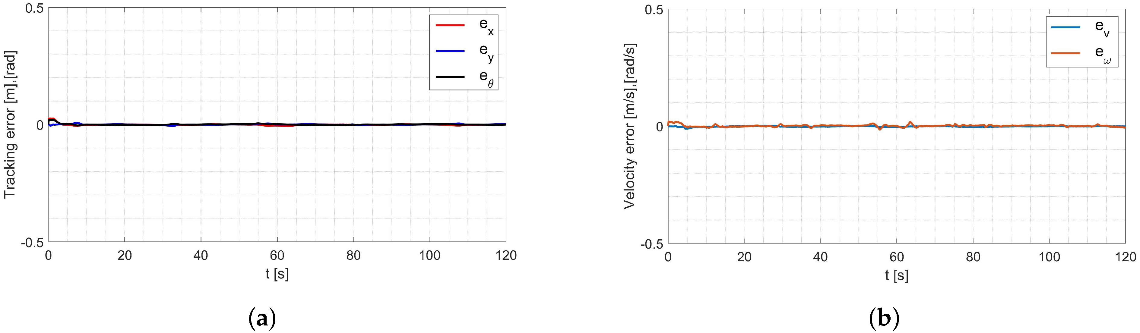
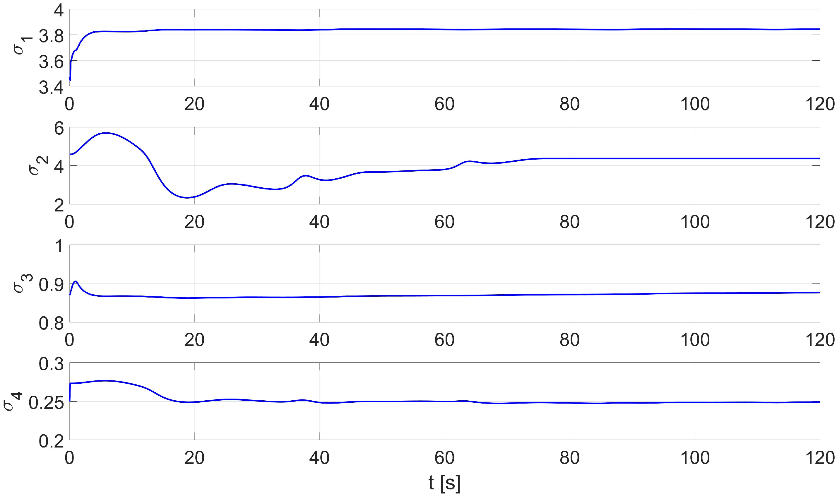
4.3. Simulation Studies of the Control System with Online Identification

Online parameters identification of the robot dynamics model was carried out based on the tracking motion simulation scheme shown in Figure 9.

In this case, an adaptive dynamic controller using the RLS method described by Equation (6) was used. The simulation was first carried out for parameters with random values equal to ${\sigma }_1=0.52,{\sigma }_2=0.23,{\sigma }_3=0.49,{\sigma }_4=0.62$. A comparison of the desired and resulting trajectories is shown in Figure 10. The position and orientation errors are shown in Figure 11a, while the velocity errors are shown in Figure 11b.

Based on the analysis of the simulation-determined errors for the RLS method with random initial parameters (Figure 11), it can be concluded that the adaptive controller, realizes control in tracking motion with position, orientation and velocity errors no greater than:

• in the x-axis direction: $e_x=0.009\left[\mathrm{m}\right]$,
• in the y-axis direction: $e_y=0.016\left[\mathrm{m}\right]$,
• orientation: $e_{\theta }=0.022\left[\mathrm{rad}\right]$,
• linear velocity $e_v=0.001\left[\frac{\mathrm{m}}{\mathrm{s}}\right]$,
• angular velocity $e_{\omega }=0.015\left[\frac{\mathrm{rad}}{\mathrm{s}}\right]$.

The regulation time for the case of an 8-shape trajectory tracking task is equal to $t_r\approx 7.8[\mathrm{s}$].

Next, the random initial parameters were replaced with average values determined using the Levenberg-Marguardt method. A comparison of the desired trajectory and obtained trajectories from this simulation is shown in Figure 12. The position and orientation errors are shown in Figure 13a, while the velocity errors are shown in Figure 13b.

Based on the analysis of the simulation-determined errors for the RLS method with the initial parameters determined by the Levenberg-Marguardt method (Figure 13), it can be concluded that the adaptive controller, realizes control in tracking motion with position, orientation and velocity errors no greater than:

• in the x-axis direction: $e_x=0.005\left[\mathrm{m}\right]$,
• in the y-axis direction: $e_y=0.002\left[\mathrm{m}\right]$,
• orientation: $e_{\theta }=0.001\left[\mathrm{rad}\right]$,
• linear velocity $e_v=0.001\left[\frac{\mathrm{m}}{\mathrm{s}}\right]$,
• angular velocity $e_{\omega }=0.017\left[\frac{\mathrm{rad}}{\mathrm{s}}\right]$.

The regulation time for the case of an 8-shape trajectory tracking task is equal to $t_r\approx 4.8\left[\mathrm{s}\right]$.

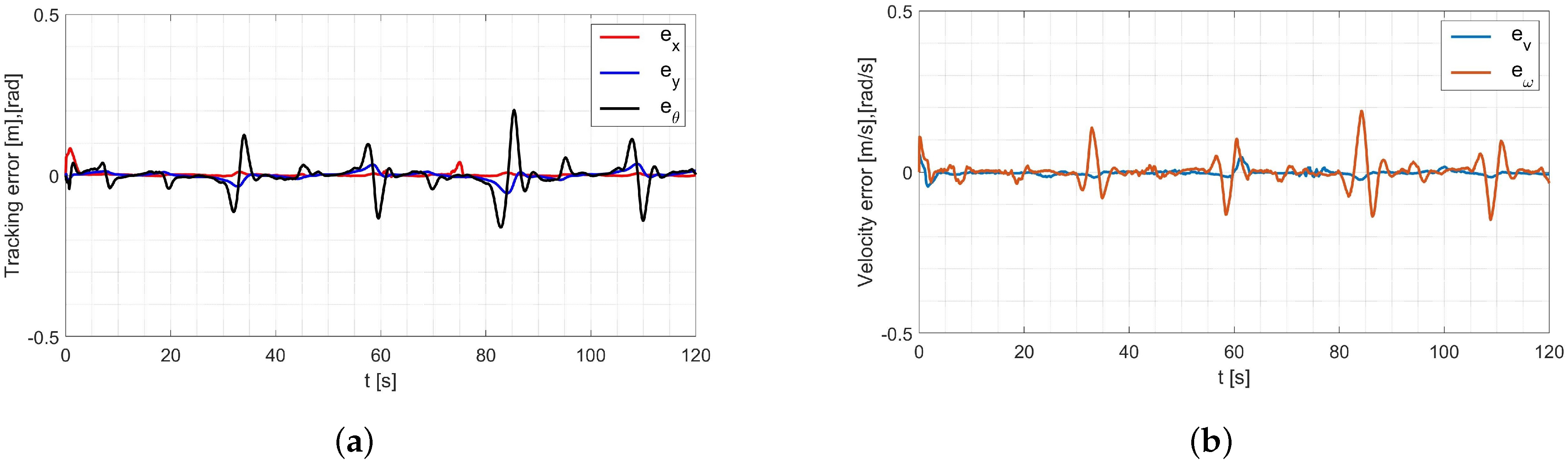
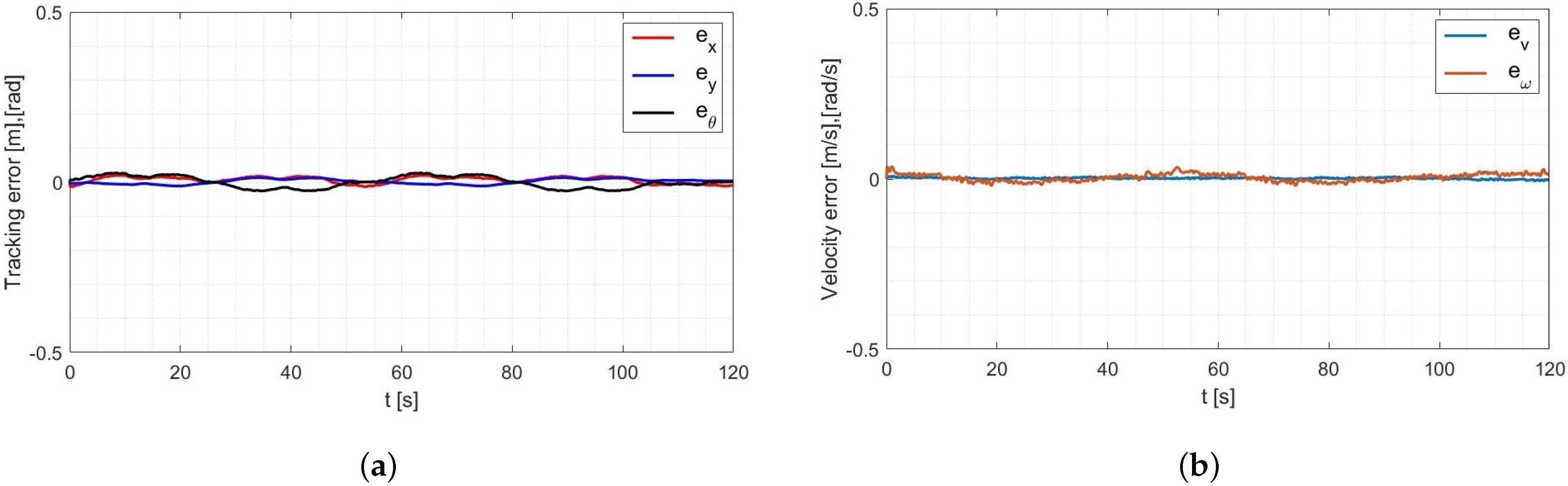
4.4. Laboratory Tests of the Control System with Parameters Identified Offline

Verification of the identified parameters was carried out by laboratory tests of the tracking motion using a real robot TURTLEBOT 2. The test used a control system, including a kinematics (10) and dynamics (12) controller, implemented using the basic elements of the Simulink package. The Simulink/ROS library and two tools (Publisher—to publish a specific type of message in a declared communication node, and Subscriber—to receive messages from the robot system transmitted in a declared communication node) were used to communicate with the robot’s operating system. Using Publisher, control signals in the form of linear and angular velocity are sent to the robot system. Using Subscriber, position and orientation are received from the robot system. A block diagram of trajectory tracking by the real TURTLEBOT 2 robot, taking into account parameters identified by offline methods, is shown in Figure 14.

The laboratory test used the average values of the model parameters shown in Table 1. A comparison of the reference and real trajectory for TURTLEBOT 2 robot with the parameters identified by the Levenberg-Marguardt method is shown in Figure 15, position and orientation errors are shown in Figure 16a, and velocity errors are shown in Figure 16b.

Based on the analysis of the errors determined in laboratory tests (Figure 16), it can be concluded that the controller, developed based on the inverse dynamics with the parameters identified by the Levenberg-Marguardt method, realizes control in tracking motion with position, orientation and velocity errors no greater than:

• in the x-axis direction: $e_x=0.033\left[\mathrm{m}\right]$,
• in the y-axis direction: $e_y=0.046\left[\mathrm{m}\right]$,
• orientation: $e_{\theta }=0.2\left[\mathrm{rad}\right]$,
• linear velocity $e_v=0.023\left[\frac{\mathrm{m}}{\mathrm{s}}\right]$,
• angular velocity $e_{\omega }=0.18\left[\frac{\mathrm{rad}}{\mathrm{s}}\right]$.

The regulation time for the case of 8-shape trajectory tracking task is equal to $t_r\approx 2.9\left[\mathrm{s}\right]$.

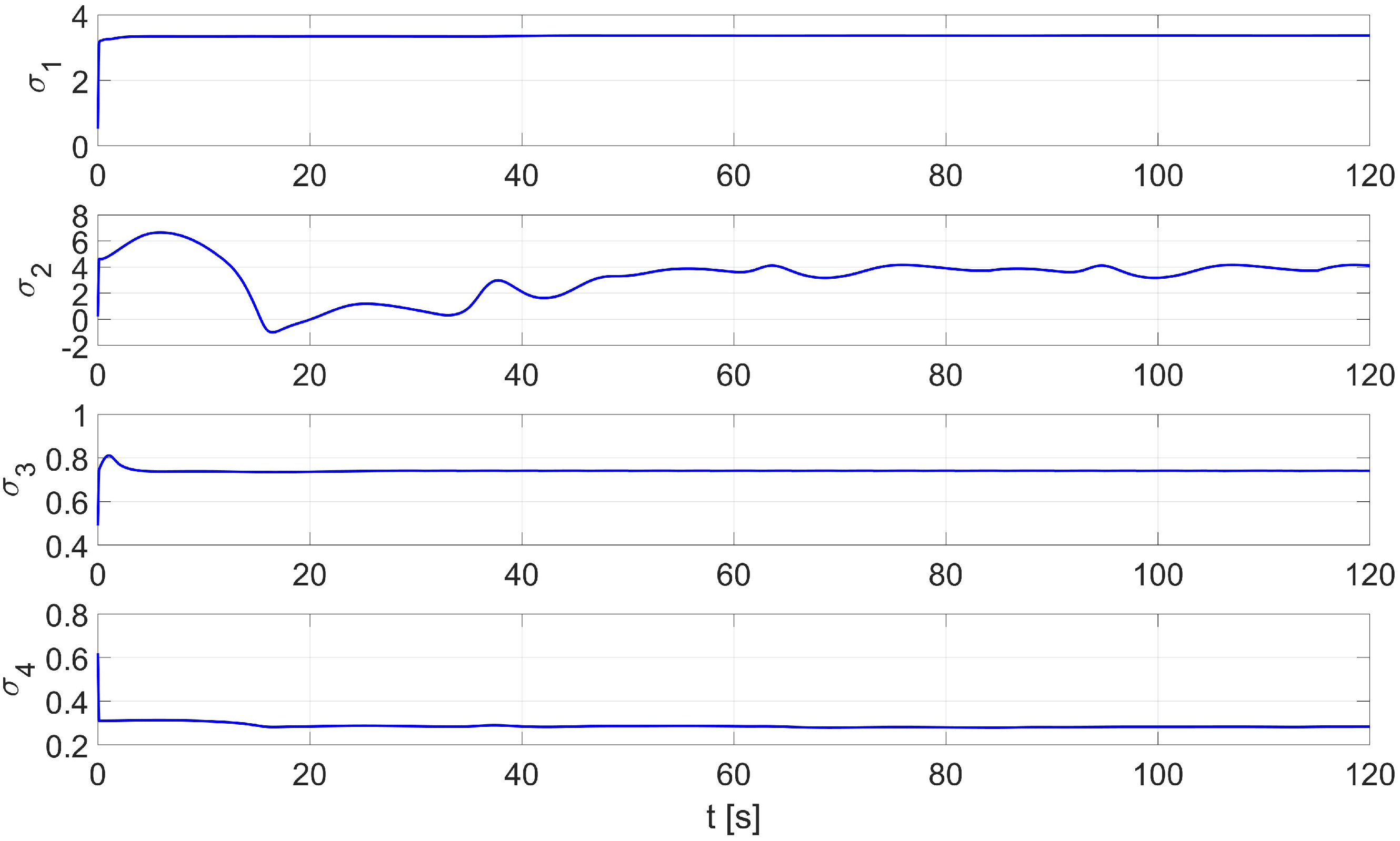
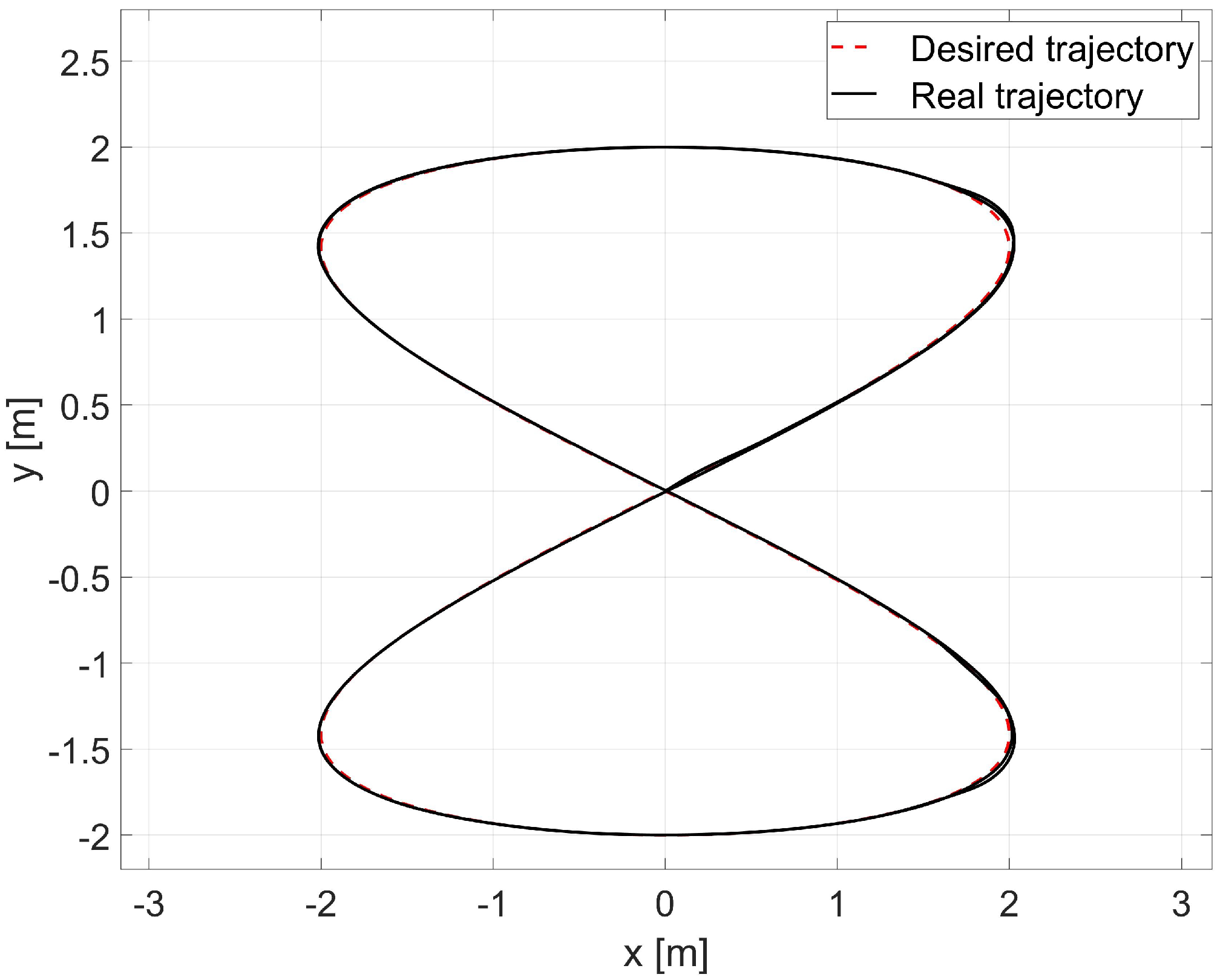
4.5. Laboratory Tests of Control System with Online Identification

The final step was to perform laboratory tests to identify the parameters of the robot’s dynamics model using online methods. A block diagram of trajectory tracking by the real TURTLEBOT 2 robot including the adaptive controller is shown in Figure 17.

The simulation was first carried out for random starting parameters with values of ${\sigma }_1=0.52,{\sigma }_2=0.23,{\sigma }_3=0.49,{\sigma }_4=0.62$. A comparison of the desired and resulting trajectories is shown in Figure 18. Position and orientation errors are shown in Figure 19a, while speed errors are shown in Figure 19b. The distribution of parameters identified during movement is shown in Figure 20.

Based on the analysis of the errors determined during the laboratory test for the RLS method with random initial parameters (Figure 19), it can be concluded that the adaptive controller, realizes control in tracking motion with position, orientation and velocity errors no greater than:

• in the x-axis direction: $e_x=0.021\left[\mathrm{m}\right]$,
• in the y-axis direction: $e_y=0.013\left[\mathrm{m}\right]$,
• orientation: $e_{\theta }=0.025\left[\mathrm{rad}\right]$,
• linear velocity $e_v=0.011\left[\frac{\mathrm{m}}{\mathrm{s}}\right]$,
• angular velocity $e_{\omega }=0.033\left[\frac{\mathrm{rad}}{\mathrm{s}}\right]$.

The regulation time for the case of an 8-shape trajectory tracking task is equal to $t_r\approx 7.5\left[\mathrm{s}\right]$.

The random initial parameters were then replaced with average values determined using the Levenberg-Marguardt method. A comparison of the desired and real trajectory is shown in Figure 21. The position and orientation errors for the combination of the RLS and Levenberg-Marguardt methods are shown in Figure 22a, while the velocity errors are shown in Figure 22b. The distribution of parameters identified during movement is shown in Figure 23.

Based on the analysis of the errors determined during the laboratory test for the RLS method with the initial parameters determined by the Levenberg-Marguardt method (Figure 22), it can be concluded that the adaptive controller, realizes control in tracking motion with position, orientation and velocity errors no greater than:

• in the x-axis direction: $e_x=0.009\left[\mathrm{m}\right]$,
• in the y-axis direction: $e_y=0.008\left[\mathrm{m}\right]$,
• orientation: $e_{\theta }=0.012\left[\mathrm{rad}\right]$,
• linear velocity $e_v=0.001\left[\frac{\mathrm{m}}{\mathrm{s}}\right]$,
• angular velocity $e_{\omega }=0.033\left[\frac{\mathrm{rad}}{\mathrm{s}}\right]$.

The regulation time for the case of an 8-shape trajectory tracking task is equal to $t_r\approx 1.6\left[\mathrm{s}\right]$.

To compare the selected identification methods, all determined errors discussed in this article, are summarized in the

Table 4. A summary of the errors determined in the studies presented.

Errors	Simulation Tests			Laboratory Tests
	L-M	RLS	RLS + L-M	L-M	RLS	RLS − L-M
$e_x\left[\mathrm{m}\right]$	0.007	0.009	0.005	0.033	0.021	0.009
$e_y\left[\mathrm{m}\right]$	0.007	0.016	0.002	0.046	0.013	0.008
$e_{\theta }\left[\mathrm{rad}\right]$	0.021	0.022	0.001	0.2	0.025	0.012
$e_v\left[\frac{\mathrm{m}}{\mathrm{s}}\right]$	0.001	0.001	0.001	0.023	0.011	0.001
$e_{\omega }\left[\frac{\mathrm{rad}}{\mathrm{s}}\right]$	0.007	0.015	0.017	0.18	0.033	0.033
$t_r\left[\mathrm{s}\right]$	8.2	7.8	4.8	2.9	7.5	1.6

below:

5. Conclusions

The article presents the process of identifying the dynamics model parameters of a mobile robot on the example of the laboratory robot TURTLEBOT 2. The identification was carried out by an offline method using a preregistered trajectory and an online method—identifying the parameters during movement. The correctness of the identification process and the values of the identified parameters were checked first by simulating the robot’s tracking motion along a desired trajectory, and then by conducting laboratory tests using a real robot. By making a comparative analysis of the desired and simulation-determined trajectories, and during laboratory testing, it has been concluded that:

• all the values of the parameters identified by the selected methods are correct, and their implementation in the control system gives satisfactory results of tracking the desired trajectory;
• parameters identified by the Levenberg-Marguardt method allow trajectory tracking with a tracking error of about 30–40 [mm] and a regulation time of about 2.9 [s];
• the use of online identification by the RLS method with random initial parameters made it possible to achieve a tracking accuracy of the set trajectory of about 10–20 [mm] and a control time of 7.5 [s]; the use of adaptive technology in the control system made it possible to improve the tracking accuracy compared to the control system with constant values of the parameters of the robot model;
• The best tracking accuracy of the desired trajectory (a tracking error of about 2–5 [mm] and a regulation time of 1.6 [s]) was achieved using the RLS method with the initial parameters determined by the Levenberg-Marguardt method.

The conducted research has shown an improvement in the accuracy of trajectory tracking of AGV robots, by using a novel combination of offline and online methods proposed by authors, for the identification of mathematical model parameters. Since the identification process and control system have been developed for a differentially driven two-wheeled robot, the presented solution can be implemented to other AGV robots, with a drive system based on the one presented in the article. Since the TURTLEBOT 2 robot is not an accurate industrial unit (it is only a low-cost laboratory robot), it introduces errors in the form of vibrations and inaccuracies in measuring the rotation angle in the z-axis and y-axis (Figure 2a). Implementation of the methodology presented in this paper on a professional and more rigid robot could achieve even better accuracy in tracking the desired trajectory. The development trend toward the use of AGV robots in internal transportation and the cooperation of industrial and mobile robots in manufacturing processes in the age of Industry 4.0 confirms the advisability of the presented research and the need to develop methods to improve the accuracy of tracking the desired trajectory.

References

1. Szrek, J.; Jakubiak, J.; Zimroz, R. A Mobile Robot-Based System for Automatic Inspection of Belt Conveyors in Mining Industry. Energies 2022, 15, 327. [Google Scholar] [CrossRef]
2. Pia̧tek, Z. Mobile Industrial Robots Enters Polish Mobile Robot Market (In Polish). 2018. Available online: https://przemysl-40.pl/index.php/2018/01/11/mobile-industrial-robots-wchodzi-na-polski-rynek/ (accessed on 5 December 2022).
3. AGV, AIV, AMR, SGV—So What’s the Deal with the Nomenclature? (In Polish). Available online: http://www.mobot.pl/artykul/5095/agv-aiv-amr-sgv-czyli-o-co-chodzi-z-tym-nazewnictwem/ (accessed on 5 December 2022).
4. Jahn, U.; Heß, D.; Stampa, M.; Sutorma, A.; Röhrig, C.; Schulz, P.; Wolff, C. A Taxonomy for Mobile Robots: Types, Applications, Capabilities, Implementations, Requirements, and Challenges. Robotics 2020, 9, 109. [Google Scholar] [CrossRef]
5. SFS-EN ISO 3691-4:2020; Industrial Trucks. Safety Requirements and Verification. Part 4: Driverless Industrial Trucks and Their Systems. SFS: Singapore, 2020.
6. Vasconcelos, J.V.R.; Brandão, A.S.; Sarcinelli-Filho, M. Real-Time Path Planning for Strategic Missions. Appl. Sci. 2020, 10, 7773. [Google Scholar] [CrossRef]
7. Zhou, Z.; Zhu, P.; Zeng, Z.; Xiao, J.; Lu, H.; Zhou, Z. Robot navigation in a crowd by integrating deep reinforcement learning and online planning. Appl. Intell. 2022, 52, 15600–15616. [Google Scholar] [CrossRef]
8. Wróblewski, P. Analysis of Torque Waveforms in Two-Cylinder Engines for Ultralight Aircraft Propulsion Operating on 0W-8 and 0W-16 Oils at High Thermal Loads Using the Diamond-like Carbon Composite Coating. SAE Int. J. Engines 2021, 15, 2022. [Google Scholar] [CrossRef]
9. Chen, Y.; Xie, B.; Long, J.; Kuang, Y.; Chen, X.; Hou, M.; Gao, J.; Zhou, S.; Fan, B.; He, Y.; et al. Interfacial Laser-Induced Graphene Enabling High-Performance Liquid-Solid Triboelectric Nanogenerator. Adv. Mater. 2021, 33, 2104290. [Google Scholar] [CrossRef]
10. Siwek, M.; Besseghieur, K.; Baranowski, L. The effects of the swarm configuration and the obstacles placement on control signals transmission delays in decentralized ROS-embedded group of mobile robots. AIP Conf. Proc. 2018, 2029, 20069. [Google Scholar] [CrossRef]
11. Timofeev, A.; Daeef, F. Control of a transport robot in extreme weather based on computer vision systems. J. Phys. Conf. Ser. 2021, 2131, 32027. [Google Scholar] [CrossRef]
12. Javed, M.A.; Muram, F.U.; Punnekkat, S.; Hansson, H. Safe and secure platooning of Automated Guided Vehicles in Industry 4.0. J. Syst. Archit. 2021, 121, 102309. [Google Scholar] [CrossRef]
13. Falcó, A.; Hilario, L.; Montés, N.; Mora, M.C.; Nadal, E. A Path Planning Algorithm for a Dynamic Environment Based on Proper Generalized Decomposition. Mathematics 2020, 8, 2245. [Google Scholar] [CrossRef]
14. Sánchez-Ibáñez, J.R.; Pérez-Del-pulgar, C.J.; García-Cerezo, A. Path planning for autonomous mobile robots: A review. Sensors 2021, 21, 7898. [Google Scholar] [CrossRef] [PubMed]
15. Zhang, H.Y.; Lin, W.M.; Chen, A.X. Path planning for the mobile robot: A review. Symmetry 2018, 10, 450. [Google Scholar] [CrossRef] [Green Version]
16. Kaczmarek, W.; Borys, S.; Panasiuk, J.; Siwek, M.; Prusaczyk, P. Experimental Study of the Vibrations of a Roller Shutter Gripper. Appl. Sci. 2022, 12, 9996. [Google Scholar] [CrossRef]
17. Borys, S.; Kaczmarek, W.; Laskowski, D.; Polak, R. Experimental Study of the Vibration of the Spot Welding Gun at a Robotic Station. Appl. Sci. 2022, 12, 12209. [Google Scholar] [CrossRef]
18. Ravankar, A.; Ravankar, A.A.; Kobayashi, Y.; Hoshino, Y.; Peng, C.C. Path smoothing techniques in robot navigation: State-of-the-art, current and future challenges. Sensors 2018, 18, 3170. [Google Scholar] [CrossRef] [Green Version]
19. Wu, M.; Dai, S.L.; Yang, C. Mixed reality enhanced user interactive path planning for omnidirectional mobile robot. Appl. Sci. 2020, 10, 1135. [Google Scholar] [CrossRef] [Green Version]
20. Andreasson, H.; Saarinen, J.; Cirillo, M.; Stoyanov, T.; Lilienthal, A.J. Drive the drive: From discrete motion plans to smooth drivable trajectories. Robotics 2014, 3, 400–416. [Google Scholar] [CrossRef] [Green Version]
21. Siwek, M.; Baranowski, L.; Panasiuk, J.; Kaczmarek, W. Modeling and simulation of movement of dispersed group of mobile robots using Simscape multibody software. AIP Conf. Proc. 2019, 2078, 020045. [Google Scholar] [CrossRef]
22. Baranowski, L.; Siwek, M. Use of 3D Simulation to Design Theoretical and Real Pipe Inspection Mobile Robot Model. Acta Mech. Autom. 2018, 12, 232–236. [Google Scholar] [CrossRef] [Green Version]
23. Noh, S.; Park, J.; Park, J. Autonomous Mobile Robot Navigation in Indoor Environments: Mapping, Localization, and Planning. In Proceedings of the International Conference on Information and Communication Technology Convergence, Jeju, Republic of Korea, 21–23 October 2020; pp. 908–913. [Google Scholar] [CrossRef]
24. Besseghieur, K.L.; Trebinski, R.; Kaczmarek, W.; Panasiuk, J. Trajectory tracking control for a nonholonomic mobile robot under ROS. J. Phys. Conf. Ser. 2018, 1016, 12008. [Google Scholar] [CrossRef] [Green Version]
25. Gonçalves, F.; Ribeiro, T.; Ribeiro, A.F.; Lopes, G.; Flores, P. A Recursive Algorithm for the Forward Kinematic Analysis of Robotic Systems Using Euler Angles. Robotics 2022, 11, 15. [Google Scholar] [CrossRef]
26. Groves, K.; Hernandez, E.; West, A.; Wright, T.; Lennox, B. Robotic exploration of an unknown nuclear environment using radiation informed autonomous navigation. Robotics 2021, 10, 78. [Google Scholar] [CrossRef]
27. Wróblewski, P. Investigation of energy losses of the internal combustion engine taking into account the correlation of the hydrophobic and hydrophilic. Energy 2023, 264, 126002. [Google Scholar] [CrossRef]
28. Panasiuk, J.; Siwek, M.; Kaczmarek, W.; Borys, S.; Prusaczyk, P. The concept of using the mobile robot for telemechanical wires installation in pipelines. AIP Conf. Proc. 2018, 2029, 020054. [Google Scholar] [CrossRef]
29. Khosla, P.K.; Kanade, T. Parameter Identification of Robot Dynamics. In Proceedings of the 24th IEEE Conference on Decision and Control, Fort Lauderdale, FL, USA, 11–13 December 1985; pp. 1754–1760. [Google Scholar] [CrossRef]
30. Gautier, M.; Janot, A.; Vandanjon, P.O. A new closed-loop output error method for parameter identification of robot dynamics. IEEE Trans. Control Syst. Technol. 2013, 21, 428–444. [Google Scholar] [CrossRef] [Green Version]
31. Briot, S.; Krut, S.; Gautier, M. Dynamic Parameter Identification of Overactuated Parallel Robots. J. Dyn. Syst. Meas. Control. Trans. ASME 2015, 137, 111002. [Google Scholar] [CrossRef]
32. Lomakin, A.; Deutscher, J. Identification of dynamic parameters for rigid robots based on polynomial approximation. In Proceedings of the IEEE/RSJ International Conference on Intelligent Robots and Systems, Las Vegas, NV, USA, 24 October 2020–24 January 2021; pp. 7271–7278. [Google Scholar] [CrossRef]
33. Uddin, N. Adaptive control system design for two-wheeled robot stabilization. In Proceedings of the 12th South East Asian Technical University Consortium, Yogyakarta, Indonesia, 12–13 March 2018; pp. 1–5. [Google Scholar] [CrossRef]
34. Al-Jlailaty, H.; Jomaa, H.; Daher, N.; Asmar, D. Balancing a Two-Wheeled Mobile Robot using Adaptive Control. In Proceedings of the 2018 IEEE International Multidisciplinary Conference on Engineering Technology, Beirut, Lebanon, 14–16 November 2018; pp. 1–7. [Google Scholar] [CrossRef]
35. Zhai, J.; Song, Z. Adaptive sliding mode trajectory tracking control for wheeled mobile robots. Int. J. Control 2019, 92, 2255–2262. [Google Scholar] [CrossRef]
36. Chen, Y.; Li, Z.; Kong, H.; Ke, F. Model predictive tracking control of nonholonomic mobile robots with coupled input constraints and unknown dynamics. IEEE Trans. Ind. Inform. 2019, 15, 3196–3205. [Google Scholar] [CrossRef]
37. Al-Mayyahi, A.; Wang, W.; Birch, P. Adaptive neuro-fuzzy technique for autonomous ground vehicle navigation. Robotics 2014, 3, 349–370. [Google Scholar] [CrossRef] [Green Version]
38. Bouzoualegh, S.; Guechi, E.H.; Kelaiaia, R. Model Predictive Control of a Differential-Drive Mobile Robot. Acta Univ. Sapientiae Electr. Mech. Eng. 2018, 10, 20–41. [Google Scholar] [CrossRef] [Green Version]
39. Zhang, K.; Sun, Q.; Shi, Y. Trajectory Tracking Control of Autonomous Ground Vehicles Using Adaptive Learning MPC. IEEE Trans. Neural Netw. Learn. Syst. 2021, 32, 5554–5564. [Google Scholar] [CrossRef]
40. Wu, W.; You, J.; Zhang, Y.; Li, M.; Su, K. Parameter Identification of Spatial-Temporal Varying Processes by a Multi-Robot System in Realistic Diffusion Fields. Robotica 2021, 39, 842–861. [Google Scholar] [CrossRef]
41. Xu, X.; Liu, X.; Zhao, B.; Yang, B. An extensible positioning system for locating mobile robots in unfamiliar environments. Sensors 2019, 19, 4025. [Google Scholar] [CrossRef] [Green Version]
42. Li, L.; Liu, Y.H.; Jiang, T.; Wang, K.; Fang, M. Adaptive Trajectory Tracking of Nonholonomic Mobile Robots Using Vision-Based Position and Velocity Estimation. IEEE Trans. Cybern. 2018, 48, 571–582. [Google Scholar] [CrossRef] [PubMed]
43. Alatise, M.; Hancke, G. Pose Estimation of a Mobile Robot Based on Fusion of IMU Data and Vision Data Using an Extended Kalman Filter. Sensors 2017, 17, 2164. [Google Scholar] [CrossRef]
44. Liu, Y.; Zhao, C.; Ren, M. An Enhanced Hybrid Visual–Inertial Odometry System for Indoor Mobile Robot. Sensors 2022, 22, 2930. [Google Scholar] [CrossRef]
45. Robot Operating System. Available online: https://www.roscomponents.com/en/mobile-robots/9-turtlebot-2.html (accessed on 5 December 2022).
46. Rivera, Z.B.; De Simone, M.C.; Guida, D. Unmanned Ground Vehicle Modelling in Gazebo/ROS-Based Environments. Machines 2019, 7, 42. [Google Scholar] [CrossRef] [Green Version]
47. Zhao, J.; Liu, S.; Li, J. Research and Implementation of Autonomous Navigation for Mobile Robots Based on SLAM Algorithm under ROS. Sensors 2022, 22, 4172. [Google Scholar] [CrossRef]
48. Chen, C.S.; Lin, C.J.; Lai, C.C.; Lin, S.Y. Velocity Estimation and Cost Map Generation for Dynamic Obstacle Avoidance of ROS Based AMR. Machines 2022, 10, 501. [Google Scholar] [CrossRef]
49. Giergiel, M.; Malka, P. Modelowanie Kinematyki I Dynamiki Mobilnego Minirobota. Model. Inżynierskie 2006, 157–162. [Google Scholar]
50. Giergiel, M.J.; Hendzel, Z.; Żylski, W. Modelowanie i Sterowanie Mobilnych Robotów Kołowych; Wydawnictwo Naukowe PWN: Warszawa, Poland, 2013; p. 257. [Google Scholar]
51. Malka, P. Pozycjonowanie i Nada̧żanie Minirobota Kołowego; AGH: Kraków, Poland, 2007. [Google Scholar]
52. Siegwart, R.; Nourbakhsh, I.R.; Scaramuzza, D. Introduction to Autonomous Mobile Robots; The MIT Press: Cambridge, MA, USA, 2011; Volume 49, pp. 49–1492. [Google Scholar] [CrossRef] [Green Version]
53. Nascimento Martins, F.; Santos Brandão, A. Motion Control and Velocity-Based Dynamic Compensation for Mobile Robots. In Applications of Mobile Robots; IntechOpen: London, UK, 2019. [Google Scholar] [CrossRef] [Green Version]
54. Das, T.; Kar, I.N. Design and implementation of an adaptive fuzzy logic-based controller for wheeled mobile robots. IEEE Trans. Control Syst. Technol. 2006, 14, 501–510. [Google Scholar] [CrossRef]
55. Hendzel, Z.; Rykała, Ł. Modelling of dynamics of a wheeled mobile robot with mecanum wheels with the use of lagrange equations of the second kind. Int. J. Appl. Mech. Eng. 2017, 22, 81–99. [Google Scholar] [CrossRef] [Green Version]
56. Ahmad Abu Hatab, R.D. Dynamic Modelling of Differential-Drive Mobile Robots using Lagrange and Newton-Euler Methodologies: A Unified Framework. Adv. Robot. Autom. 2013, 2, 1–7. [Google Scholar] [CrossRef] [Green Version]
57. De La Cruz, C.; Carelli, R. Dynamic model based formation control and obstacle avoidance of multi-robot systems. Robotica 2008, 26, 345–356. [Google Scholar] [CrossRef]
58. Martins, F.N.; Sarcinelli-Filho, M.; Carelli, R. A Velocity-Based Dynamic Model and Its Properties for Differential Drive Mobile Robots. J. Intell. Robot. Syst. Theory Appl. 2017, 85, 277–292. [Google Scholar] [CrossRef]
59. Zhang, Y.; Hong, D.; Chung, J.H.; Velinsky, S.A. Dynamic model based robust tracking control of a differentially steered wheeled mobile robot. In Proceedings of the American Control Conference, Philadelphia, PA, USA, 26–26 June 1998; Volume 2, pp. 850–855. [Google Scholar] [CrossRef]
60. Gratton, S.; Lawless, A.S.; Nichols, N.K. Approximate Gauss-newton methods for nonlinear least squares problems. SIAM J. Optim. 2007, 18, 106–132. [Google Scholar] [CrossRef] [Green Version]
61. Moré, J.J. The Levenberg-Marquardt algorithm: Implementation and theory. In Numerical Analysis; Springer: Berlin/Heidelberg, Germany, 1978; pp. 105–116. [Google Scholar] [CrossRef] [Green Version]
62. Palacín, J.; Rubies, E.; Clotet, E. Systematic Odometry Error Evaluation and Correction in a Human-Sized Three-Wheeled Omnidirectional Mobile Robot Using Flower-Shaped Calibration Trajectories. Appl. Sci. 2022, 12, 2606. [Google Scholar] [CrossRef]
63. Klančar, G.; Matko, D.; Blažič, S. Mobile robot control on a reference path. In Proceedings of the 2005 IEEE International Symposium on, Mediterrean Conference on Control and Automation Intelligent Control, Limassol, Cyprus, 27–29 June 2005; Volume 2005, pp. 1343–1348. [Google Scholar] [CrossRef]
Figure 1. The number of mobile robots used in industry [2].
Materials 16 00683 g001
Figure 2. (a) Isometric view of the TURTLEBOT 2 robot with the coordinate system; (b) kinematic structure to determine the kinematic model.
Materials 16 00683 g002
Figure 3. TURTLEBOT 2 robot schematic for developing the dynamics model.
Materials 16 00683 g003
Figure 4. An example of the RLS identification process (test No. 1 from Table 2).
Materials 16 00683 g004
Figure 5. An example of the identification process using the Levenberg-Marguardt-assisted RLS method.
Materials 16 00683 g005
Figure 7. Comparison of the desired trajectory and that obtained by simulation for the Levenberg- Marguardt method.
Materials 16 00683 g007
Figure 8. Errors for the Levenberg-Marguardt method: (a) reference trajectory tracking, (b) velocity.
Materials 16 00683 g008
Figure 9. Block diagram of the TURTLEBOT 2 robot’s tracking motion simulation.
Materials 16 00683 g009
Figure 10. Comparison of reference and actual trajectories in a simulation test for the RLS method with random initial parameters.
Materials 16 00683 g010
Figure 11. Errors for the RLS method with random initial parameters: (a) tracking the reference trajectory (b) velocity.
Materials 16 00683 g011
Figure 12. Comparison of the reference trajectory and the one obtained by simulation for the combination of RLS and Levenberg-Marguardt methods.
Materials 16 00683 g012
Figure 13. Errors for the RLS method with initial parameters determined by the Levenberg-Marguardt method: (a) tracking the reference trajectory (b) velocity.
Materials 16 00683 g013
Figure 14. Block diagram of the real TURTLEBOT 2 robot’s tracking motion control system.
Materials 16 00683 g014
Figure 15. Comparison of reference and real trajectories in a laboratory test.
Materials 16 00683 g015
Figure 16. Errors for the Levenberg-Marguardt method: (a) tracking the reference trajectory (b) velocity.
Materials 16 00683 g016
Figure 17. Block diagram of a real robot tracking motion with an adaptive controller.
Materials 16 00683 g017
Figure 18. Comparison of reference and real trajectories in a laboratory test of RLS identification with random values of initial parameters.
Materials 16 00683 g018
Figure 19. The errors of: (a) tracking the reference trajectory (b) speed.
Materials 16 00683 g019
Figure 20. Distribution of parameters identified online by the RLS method with random values of initial parameters in the laboratory test.
Materials 16 00683 g020
Figure 21. Comparison of the reference and real trajectories in the laboratory test of identification by the RLS method with the values of the initial parameters determined by the Levenberg-Marguardt method.
Materials 16 00683 g021
Figure 22. Errors for the RLS method with initial parameters determined by the Levenberg-Marguardt method: (a) tracking of the reference trajectory, (b) velocity.
Materials 16 00683 g022
Figure 23. Distribution of parameters identified online by the RLS method with random values of initial parameters in the laboratory test.
Materials 16 00683 g023