
Experimental and Numerical Analysis of Fracture Mechanics Behavior of Heterogeneous Zones in S690QL1 Grade High Strength Steel (HSS) Welded Joint


Abstract
:1. Introduction
2. Materials and Experimental Methods
2.1. Materials
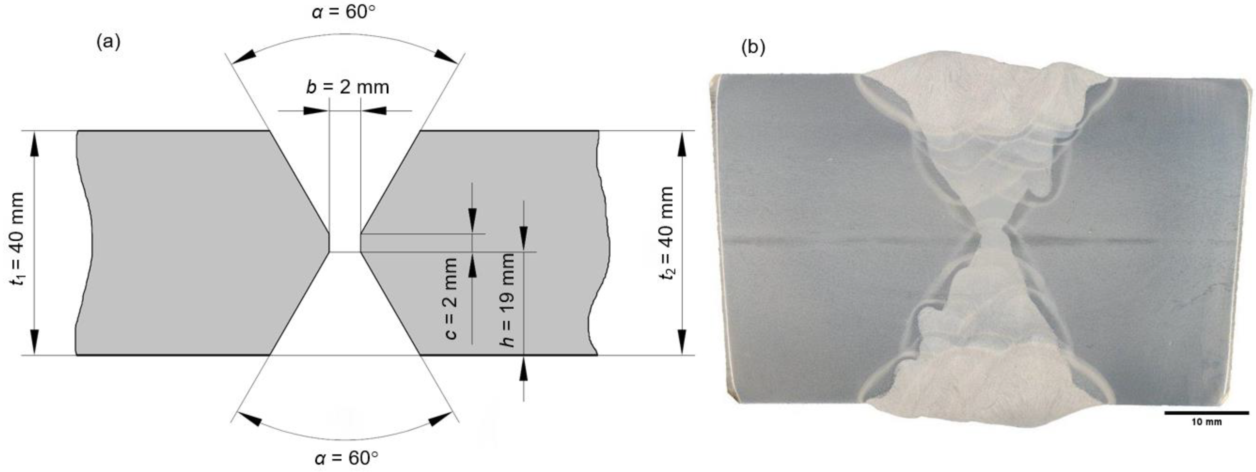
2.2. Welded Joint and Process
2.3. Test Plan
- 1—Mini tensile specimens (MTS) testing
- 2—Fracture mechanics testing, fractographic analysis
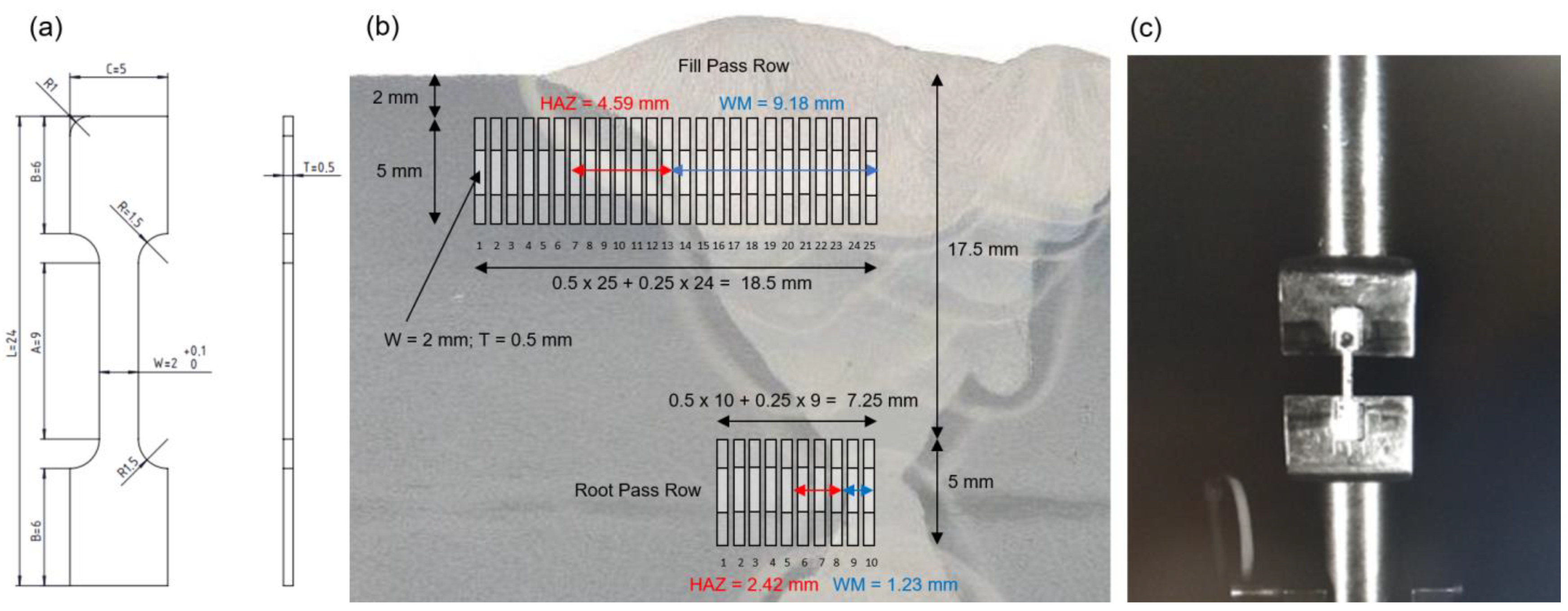
2.4. Mini Tensile Specimens (MTS) Testing
2.5. Fracture Mechanics Testing
2.6. Fractography
3. Numerical Methods
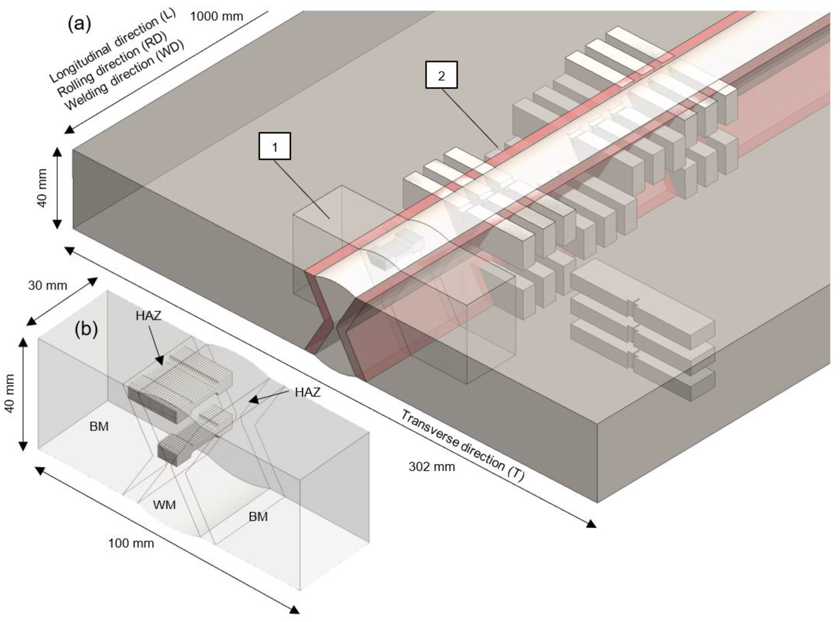
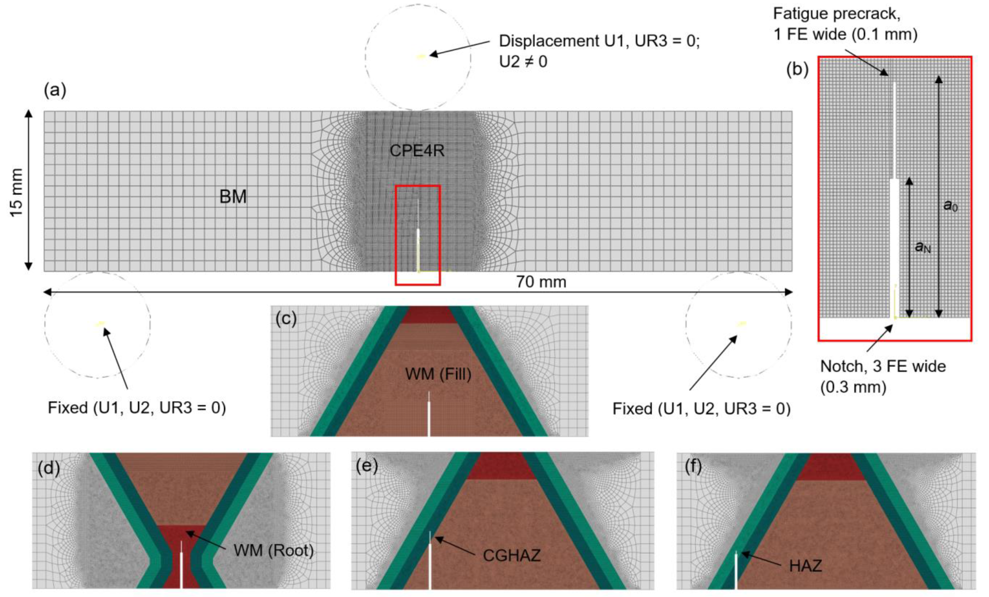
3.1. Welded Joint Simplified Model
3.2. Test Specimen Numerical Models
3.3. Ductile Damage
4. Results
4.1. Mini Tensile Specimens (MTS) Testing
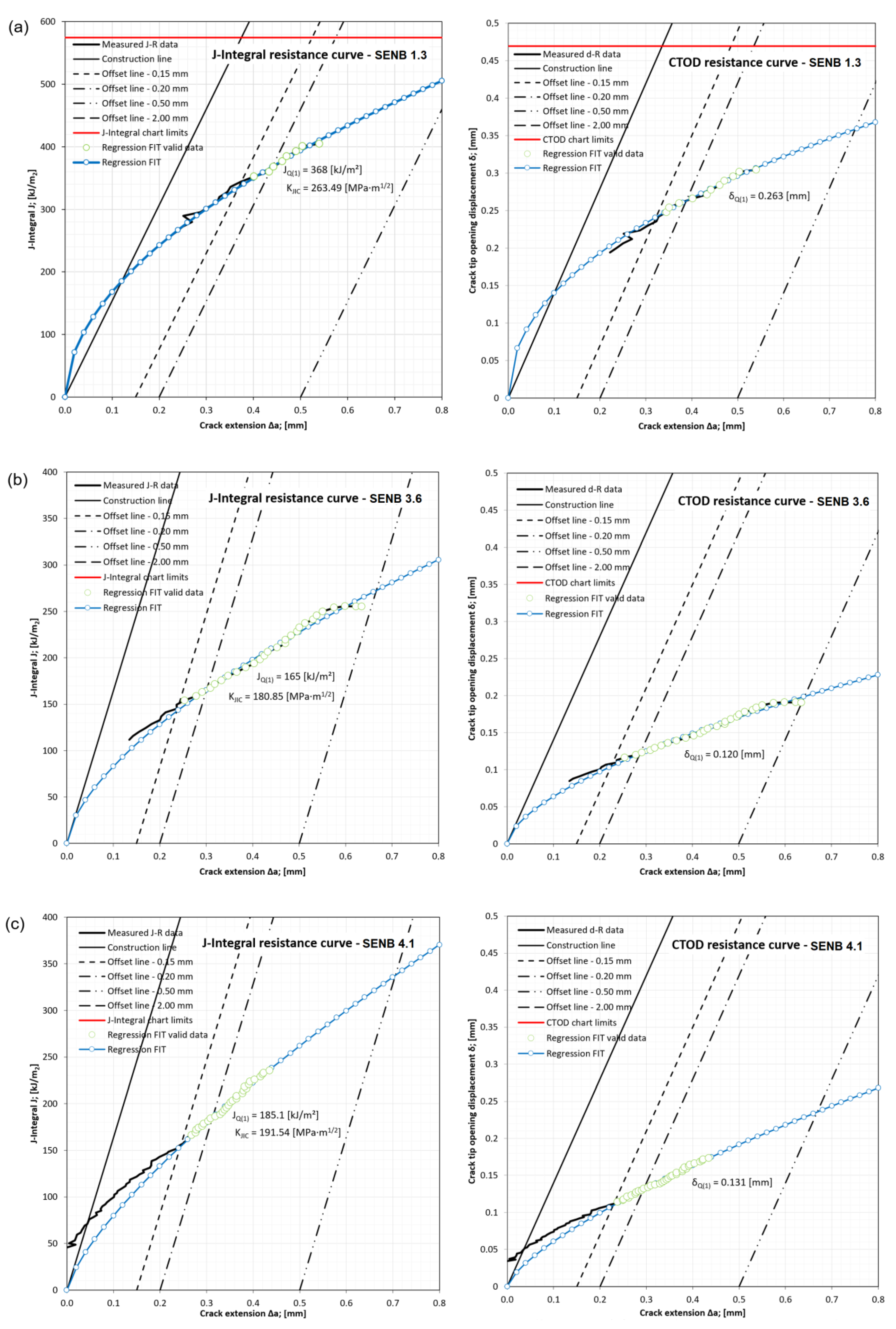
4.2. Fracture Mechanics Testing—Fracture Toughness
4.3. Fractography
4.4. Ductile Damage Material Parameters
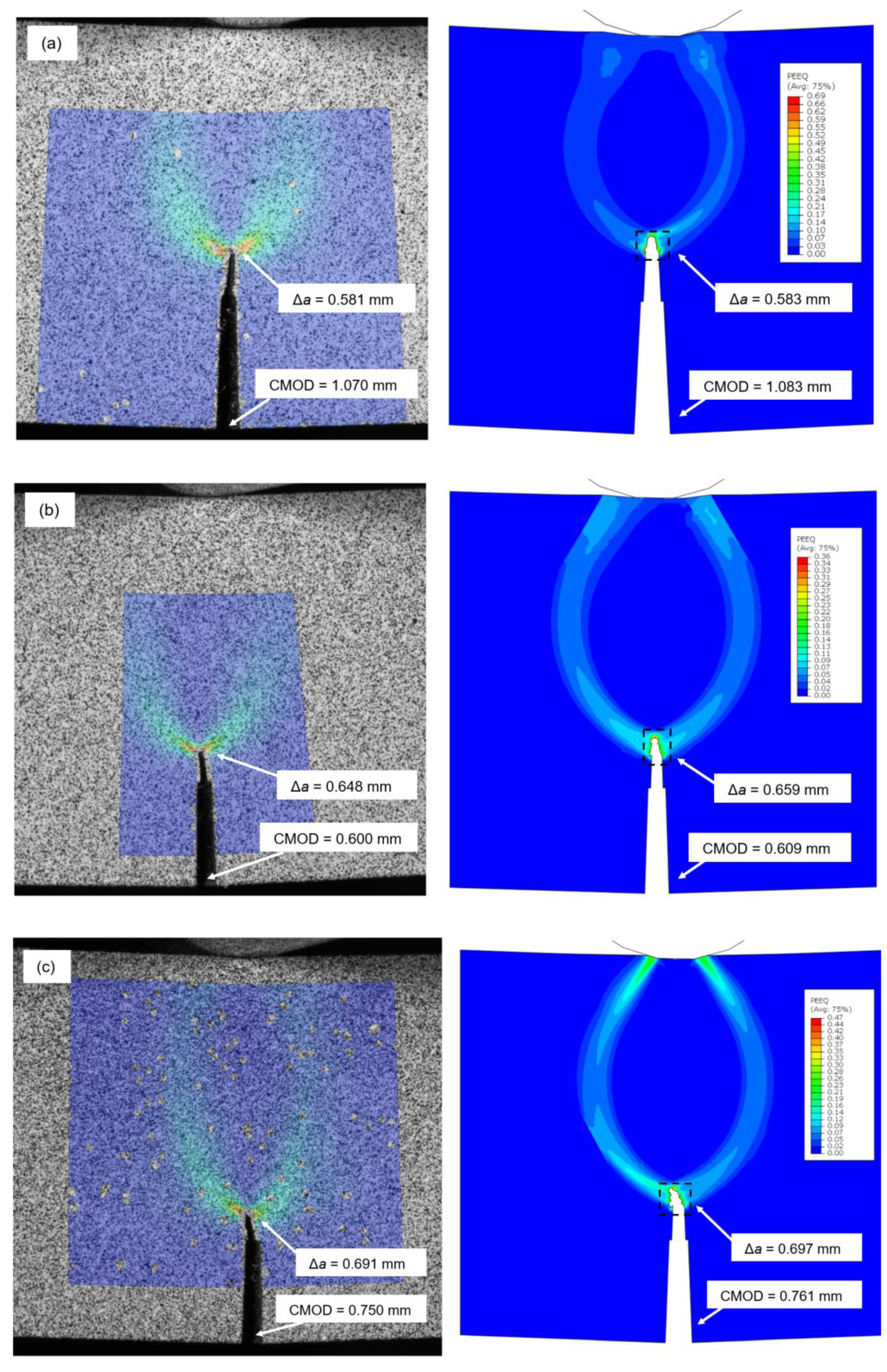
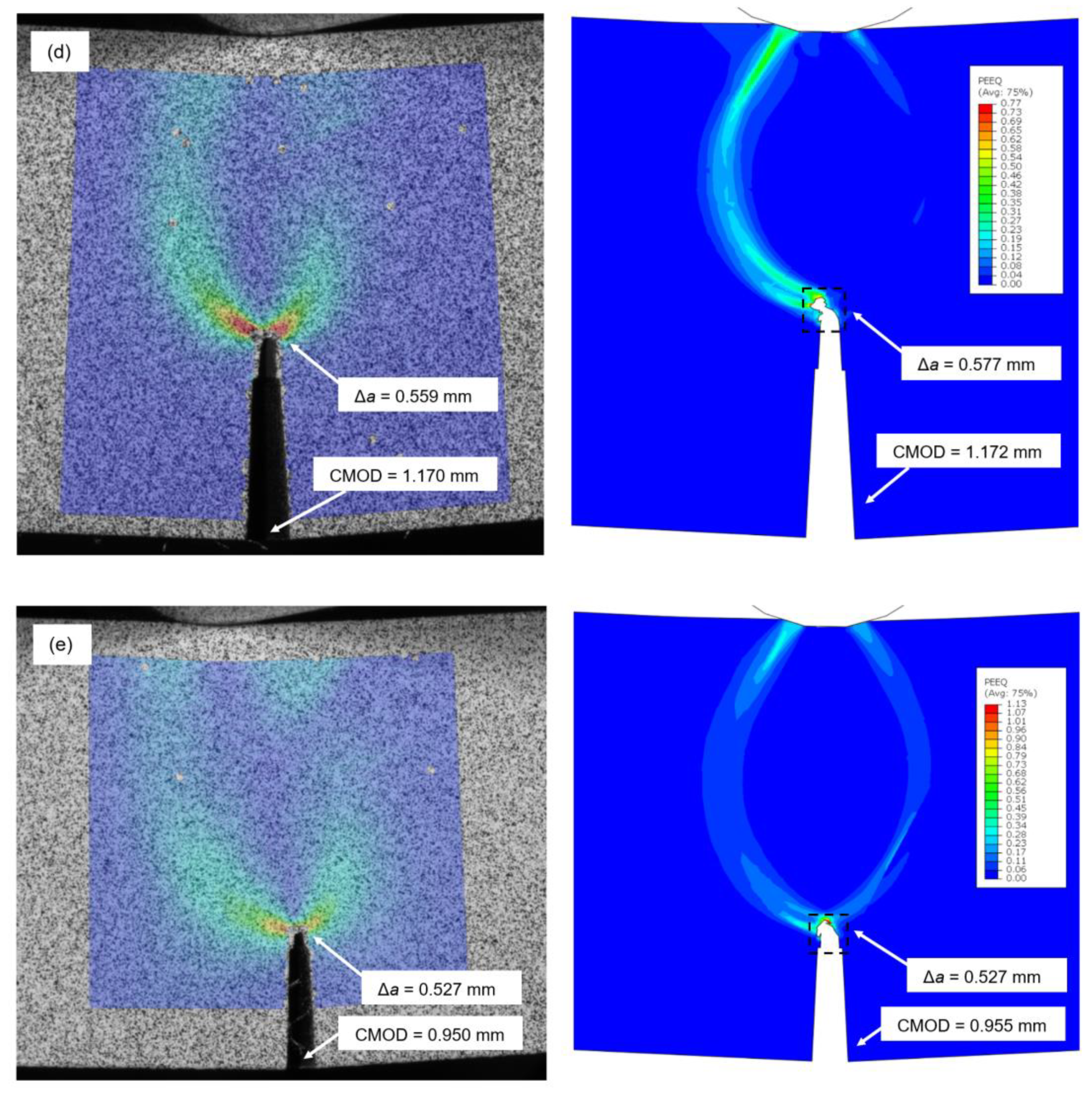
4.5. Numerical Analysis
5. Conclusions
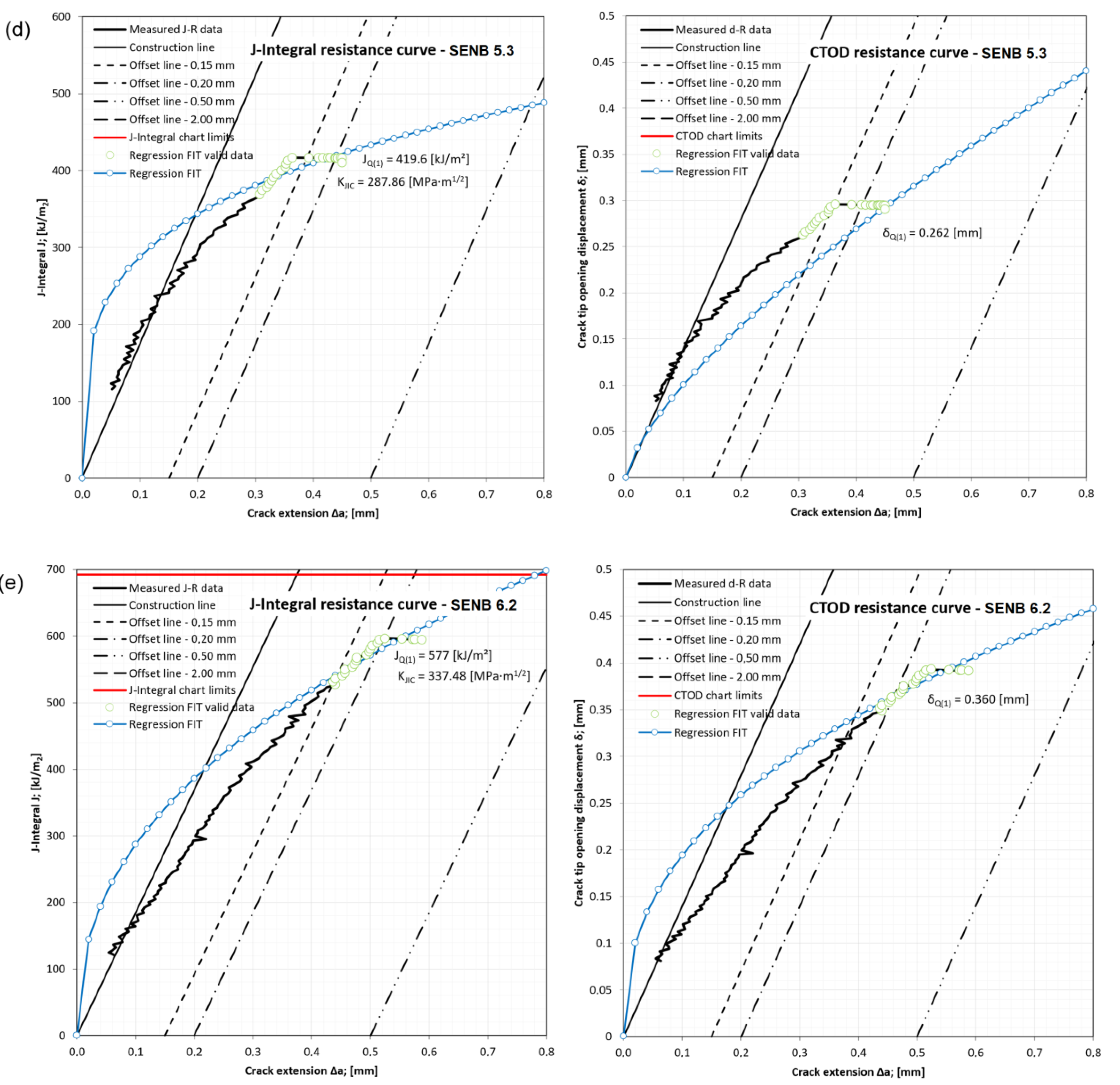
- Examining the crack extension Δa trend throughout materials of different welded joint zones, based on averaged values, it can be concluded that, starting from the longest crack, crack extension lengths are: WM (Fill) with Δa = 0.800 mm; WM (Root) with Δa = 0.617 mm; CGHAZ with Δa = 0.604 mm; HAZ with Δa = 0.551 mm; BM with Δa = 0.504 mm. All values are given in Table 7.
- Examining the fracture toughness testing parameters JIC, KJIC and δIC trends throughout materials of different welded joint zones, based on averaged values, it can be concluded that, starting from the highest values, all of the values are: HAZ with JIC = 590.940 kJ/m2, KJIC = 341.146 MPa∙m1/2, δIC = 0.386 mm; CGHAZ with JIC = 415.067 kJ/m2, KJIC = 286.193 MPa∙m1/2, δIC = 0.266 mm; BM with JIC = 383.583 kJ/m2, KJIC = 266.962 MPa∙m1/2, δIC = 0.277 mm; WM (Root) with JIC = 189.333 kJ/m2, KJIC = 193.457 MPa∙m1/2, δIC = 0.134 mm; WM (Fill) with JIC = 175.367 kJ/m2, KJIC = 184.851 MPa∙m1/2, δIC = 0.127 mm. All values are given in Table 12.
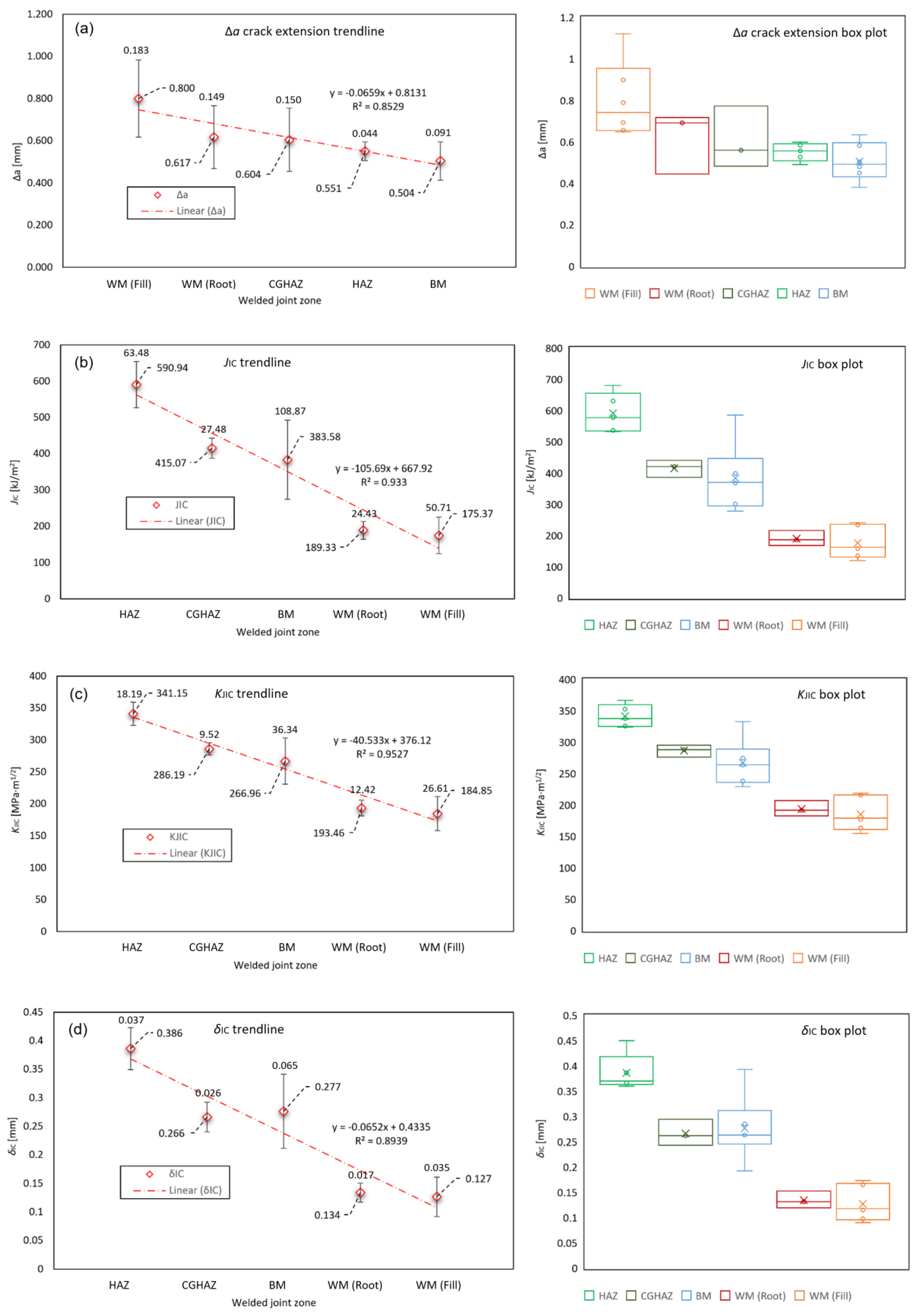
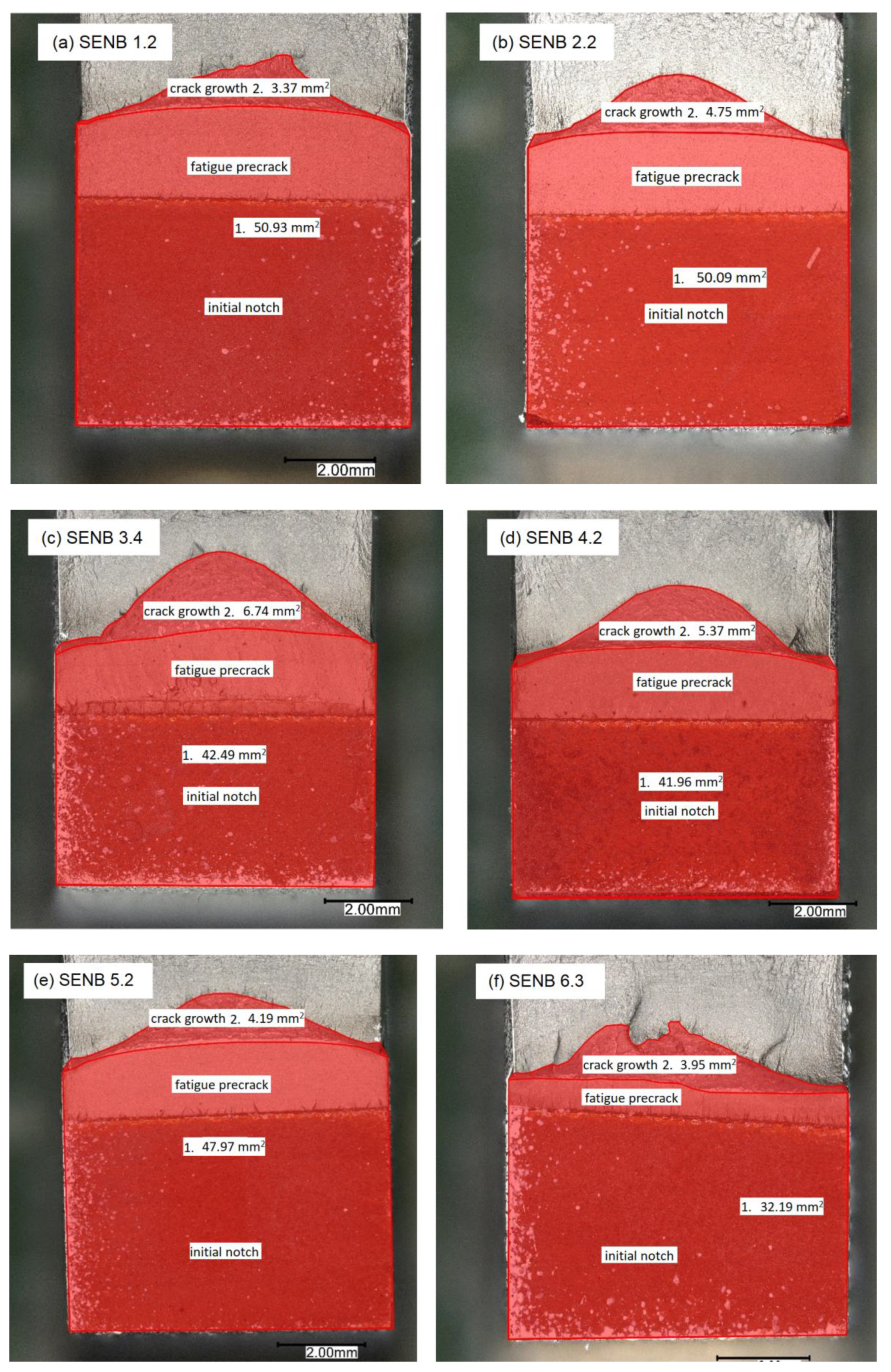
- Overall fracture behavior of welded joint materials is determined, with crack growth being most significant in WM (Fill) material with largest crack extension and lowest fracture resistance values (Δa = max.; JIC, KJIC, δIC = min.) and least significant in HAZ material (Δa = 2nd min. after BM.; JIC, KJIC, δIC = max.).
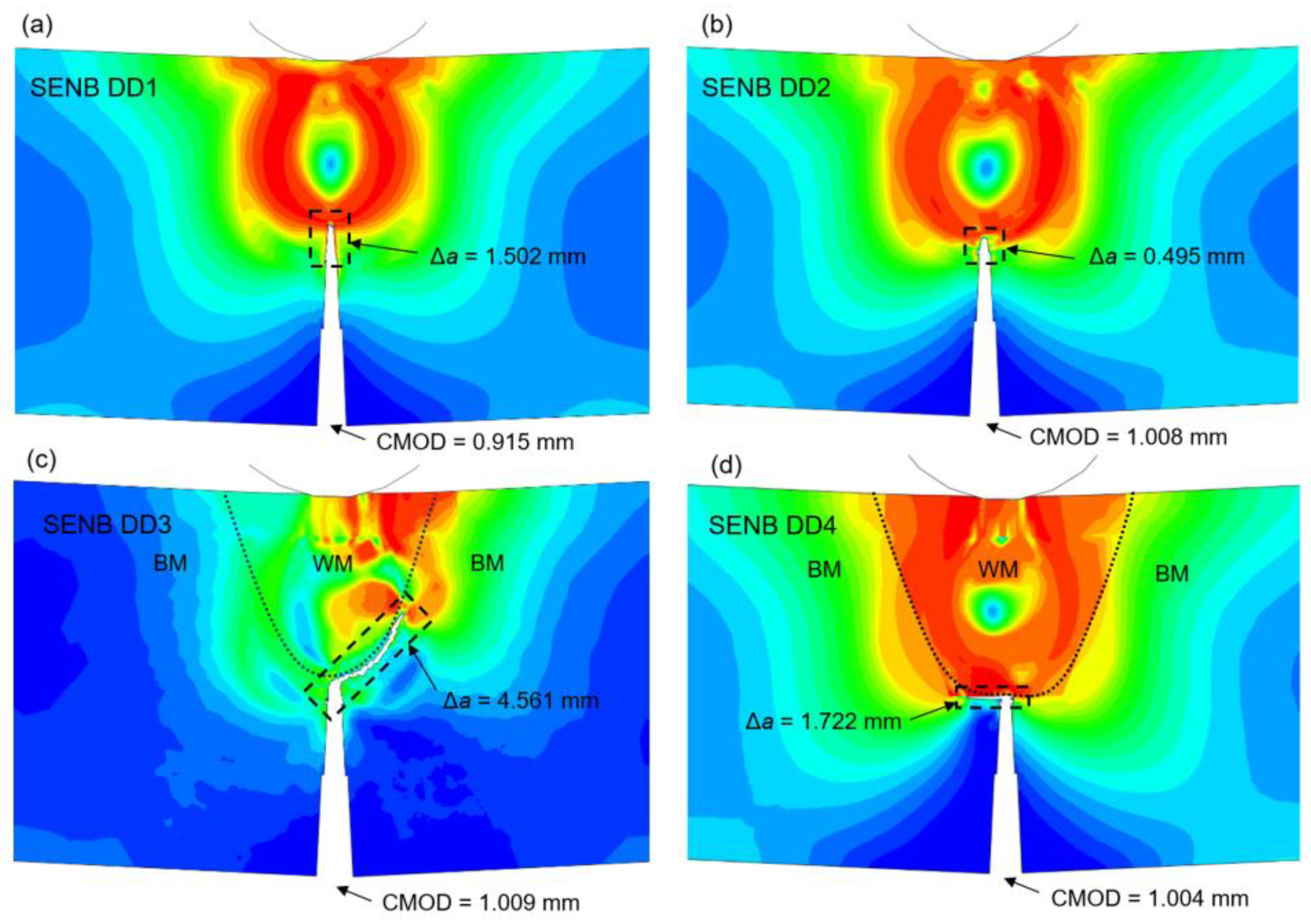
- Elasto-plastic material model with ductile damage is able to describe the fracture behavior of heterogeneous material volumes, e.g., welded joints. Crack dimensions, growth and direction can be accurately modelled through input of ductile damage material parameters: fracture strain and damage evolution displacement at failure . The comparison of several SENB DD (Ductile Damage) specimens damage behavior, with different material parameters, is shown in Figure 13.
Author Contributions
Funding
Institutional Review Board Statement
Informed Consent Statement
Data Availability Statement
Acknowledgments
Conflicts of Interest
References
- Easterling, K.E. Introduction to the Physical Metallurgy of Welding, 2nd ed.; Butterworth-Heinemann: London, UK, 1992. [Google Scholar]
- Nippes, E.F. The weld heat-affected zone. Weld. J. 1959, 38, 1–17. [Google Scholar]
- Davis, C.L.; King, J.E. Effect of cooling rate on intercritically reheated microstructure and toughness in high strength low alloy steel. Mater. Sci. Technol. 1993, 9, 8–15. [Google Scholar] [CrossRef]
- Tomerlin, D.; Marić, D.; Kozak, D.; Samardžić, I. Post-Weld Heat Treatment of S690QL1 Steel Welded Joints: Influence on Microstructure, Mechanical Properties and Residual Stress. Metals 2023, 13, 999. [Google Scholar] [CrossRef]
- Karkhin, V.A. Prediction of Local Microstructure and Mechanical Properties of Welded Joint Metal with Allowance for Its Thermal Cycle. In Thermal Processes in Welding; Engineering Materials; Springer: Singapore, 2019; pp. 441–470. [Google Scholar] [CrossRef]
- Maurer, W.; Ernst, W.; Rauch, R.; Vallant, R.; Enzinger, N. Evaluation of the factors influencing the strength of HSLA steel weld joint with softened HAZ. Weld. World 2015, 59, 809–822. [Google Scholar] [CrossRef]
- ASTM E8/E8M-16a; Standard Test Methods for Tension Testing of Metallic Materials. ASTM International: West Conshohocken, PA, USA, 2016.
- Starčevič, L.; Gubeljak, N.; Predan, J. The Numerical Modelling Approach with a Random Distribution of Mechanical Properties for a Mismatched Weld. Materials 2021, 14, 5896. [Google Scholar] [CrossRef]
- Hertelé, S.; Bally, J.; Gubeljak, N.; Stefane, P.; Verleysen, P.; De Waele, W. Characterization of Heterogeneous Arc Welds through Miniature Tensile Testing and Vickers Hardness Mapping. Mater. Tehnol. 2016, 50, 571–574. [Google Scholar] [CrossRef]
- Hertelé, S.; Gubeljak, N.; De Waele, W. Advanced characterization of heterogeneous arc welds using micro tensile tests and a two-stage strain hardening (‘UGent’) model. Int. J. Press. Vessel. Pip. 2014, 119, 87–94. [Google Scholar] [CrossRef]
- Tomerlin, D.; Kozak, D.; Gubeljak, N.; Magić Kukulj, M. Stress-Strain Properties of HSS Steel Welded Joint Heterogeneous Structure: Experimental and Numerical Evaluation. Math. Model. Weld Phenom. 2023, 13, 413–428. [Google Scholar] [CrossRef]
- SSAB. Welding Handbook: A Guide to Better Welding of Hardox and Strenx, 2nd ed.; SSAB: Oxelösund, Sweden, 2019. [Google Scholar]
- Khurshid, M.; Barsoum, Z.; Mumtaz, N.A. Ultimate strength and failure modes for fillet welds in high strength steels. Mater. Des. 2012, 40, 36–42. [Google Scholar] [CrossRef]
- Mičian, M.; Frátrik, M.; Moravec, J.; Švec, M. Determination of Grain Growth Kinetics of S960MC Steel. Materials 2022, 15, 8539. [Google Scholar] [CrossRef]
- Štefane, P.; Hertelé, S.; Naib, S.; De Waele, W.; Gubeljak, N. Effects of Fixture Configurations and Weld Strength Mismatch on J-Integral Calculation Procedure for SE(B) Specimens. Materials 2022, 15, 962. [Google Scholar] [CrossRef] [PubMed]
- Bertolo, V.; Jiang, Q.; Terol Sanchez, M.; Riemslag, T.; Walters, C.L.; Sietsma, J.; Popovich, V. Cleavage fracture micromechanisms in simulated heat affected zones of S690 high strength steels. Mater. Sci. Eng. A 2023, 868, 144762. [Google Scholar] [CrossRef]
- Kim, J.-S.; Larrosa, N.O.; Horn, A.J.; Kim, Y.-J.; Ainsworth, R.A. Notch bluntness effects on fracture toughness of a modified S690 steel at 150 °C. Eng. Fract. Mech. 2018, 188, 250–267. [Google Scholar] [CrossRef]
- Damjanović, D.; Kozak, D.; Matvienko, Y.; Gubeljak, N. Correlation of Pipe Ring Notched Bend (PRNB) specimen and Single Edge Notch Bend (SENB) specimen in determination of fracture toughness of pipe material. Fatigue Fract. Eng. Mater. Struct. 2017, 40, 1251–1259. [Google Scholar] [CrossRef]
- Yu, W.; Fan, M.; Gao, H.; Yu, D.; Xue, F.; Chen, X. Effect of long-term aging on the fracture toughness of primary coolant piping material Z3CN20.09M. Nucl. Eng. Des. 2018, 327, 150–160. [Google Scholar] [CrossRef]
- Chai, M.; Lai, C.; Xu, W.; Song, Y.; Zhang, Z.; Duan, Q. Determination of fracture toughness of 2.25Cr1Mo0.25V steel based on acoustic emission technique. Int. J. Press. Vessel. Pip. 2023, 205, 104998. [Google Scholar] [CrossRef]
- Frómeta, D.; Parareda, S.; Lara, A.; Molas, S.; Casellas, D.; Jonsén, P.; Calvo, J. Identification of fracture toughness parameters to understand the fracture resistance of advanced high strength sheet steels. Eng. Fract. Mech. 2020, 229, 106949. [Google Scholar] [CrossRef]
- Gao, H.; Wang, W.; Wang, Y.; Zhang, B.; Li, C.-Q. A modified normalization method for determining fracture toughness of steel. Fatigue Fract. Eng. Mater. Struct. 2021, 44, 568–583. [Google Scholar] [CrossRef]
- EN 10025-6:2004; Hot Rolled Products of Structural Steel—Part 6: Technical Delivery Conditions for Flat Products of High Yield Strength Structural Steels in the Quenched and Tempered Condition. CEN: Brussels, Belgium, 2004.
- Ilsenburger Grobblech GmbH Fine-Grain Structural Steels—MAXIL® 690. Available online: https://www.ilsenburger-grobblech.de/fileadmin/footage/MEDIA/gesellschaften/ilg/dokumente/Werkstoffblaetter/Werkstoffblaetter_englisch/2022_Fine-Grain_Structural_Steels_MAXIL690.pdf (accessed on 24 June 2023).
- SSAB Strenx 700 E/F General Product Description. Available online: https://www.ssab.com/en/brands-and-products/strenx/product-offer/700/e-f (accessed on 24 June 2023).
- Böhler Welding by Voestalpine Filler Metals Bestseller for Joining Applications. Available online: https://welding-expert.com/uploads/media/Weldingguide_ENGnew.pdf (accessed on 24 June 2023).
- ISO 16834:2006; Welding Consumables—Wire Electrodes, Wires, Rods and Deposits for Gas-Shielded Arc Welding of High Strength Steels—Classification. ISO: Geneva, Switzerland, 2006.
- AWS A5.28/A5.28M:2005; Specification for Low-Alloy Steel Electrodes and Rods for Gas Shielded Arc Welding. AWS: Miami, FL, USA, 2005.
- EN-1011-2:2001; Welding—Recommendations for Welding of Metallic Materials—Part 2: Arc Welding of Ferritic Steels. CEN: Brussels, Belgium, 2001.
- EN ISO 9692-1:2003; Welding and Allied Processes—Recommendations for Joint Preparation—Part 1: Manual Metal-Arc Welding, Gas-Shielded Metal-Arc Welding, Gas Welding, TIG Welding and Beam Welding of Steels (ISO 9692-1:2003). CEN: Brussels, Belgium, 2003.
- Konjatić, P.; Katinić, M.; Kozak, D.; Gubeljak, N. Yield Load Solutions for SE(B) Fracture Toughness Specimen with I-Shaped Heterogeneous Weld. Materials 2022, 15, 214. [Google Scholar] [CrossRef]
- Hochhauser, F.; Ernst, W.; Rauch, R.; Vallant, R.; Enzinger, N. Influence of the Soft Zone on The Strength of Welded Modern Hsla Steels. Weld. World 2012, 56, 77–85. [Google Scholar] [CrossRef]
- Mičian, M.; Harmaniak, D.; Nový, F.; Winczek, J.; Moravec, J.; Trško, L. Effect of the t8/5 Cooling Time on the Properties of S960MC Steel in the HAZ of Welded Joints Evaluated by Thermal Physical Simulation. Metals 2020, 10, 229. [Google Scholar] [CrossRef]
- BS 7448-2:1997; Fracture Mechanics Toughness Test, Part-2. Method for Determination of KIc, Critical CTOD and Critical J Values of Welds in Metallic Materials. BSI Standards Limited, Chiswick Tower: London, UK, 1997.
- ASTM E1820-15; Standard Test Method for Measurement of Fracture Toughness. ASTM International: West Conshohocken, PA, USA, 2016.
- Zhu, X.-K.; Joyce, J.A. Review of fracture toughness (G, K, J, CTOD, CTOA) testing and standardization. Eng. Fract. Mech. 2012, 85, 1–46. [Google Scholar] [CrossRef]
- Hertelé, S.; De Waele, W.; Verstraete, M.; Denys, R.; O’Dowd, N. J-integral analysis of heterogeneous mismatched girth welds in clamped single-edge notched tension specimens. Int. J. Press. Vessel. Pip. 2014, 119, 95–107. [Google Scholar] [CrossRef]
- Hertelé, S.; O’Dowd, N.; Van Minnebruggen, K.; Verstraete, M.; De Waele, W. Fracture Mechanics Analysis of Heterogeneous Welds: Validation of a Weld Homogenisation Approach. Procedia Mater. Sci. 2014, 3, 1322–1329. [Google Scholar] [CrossRef]
- Souza, R.F.; Ruggieri, C.; Zhang, Z. A framework for fracture assessments of dissimilar girth welds in offshore pipelines underbending. Eng. Fract. Mech. 2016, 163, 66–88. [Google Scholar] [CrossRef]
- Katinić, M.; Turk, D.; Konjatić, P.; Kozak, D. Estimation of C* Integral for Mismatched Welded Compact Tension Specimen. Materials 2021, 14, 7491. [Google Scholar] [CrossRef]
- Bi, Y.; Yuan, X.; Hao, M.; Wang, S.; Xue, H. Numerical Investigation of the Influence of Ultimate-Strength Heterogeneity on Crack Propagation and Fracture Toughness in Welded Joints. Materials 2022, 15, 3814. [Google Scholar] [CrossRef]
- Alves, D.N.L.; Almeida, J.G.; Rodrigues, M.C. Experimental and numerical investigation of crack growth behavior in a dissimilar welded joint. Theor. Appl. Fract. Mech. 2020, 109, 102697. [Google Scholar] [CrossRef]
- Abaqus Simulia. Available online: https://www.3ds.com/products-services/simulia/products/abaqus/ (accessed on 10 July 2023).
- Abaqus Ductile Damage Model. Available online: https://abaqus-docs.mit.edu/2017/English/SIMACAEMATRefMap/simamat-c-damageevolductile.htm (accessed on 10 July 2023).
- Yang, F.; Veljkovic, M.; Liu, Y. Ductile damage model calibration for high-strength structural steels. Constr. Build. Mater. 2020, 263, 120632. [Google Scholar] [CrossRef]
- Xue, L. Ductile Fracture Modeling: Theory, Experimental Investigation and Numerical Verification. Ph.D. Thesis, Massachusetts Institute of Technology, Cambridge, MA, USA, 2007. [Google Scholar]
- Song, W.; Liu, X.; Berto, F.; Xu, J.; Fang, H. Numerical simulation of prestrain history effect on ductile crack growth in mismatched welded joints. Fatigue Fract. Eng. Mater. Struct. 2017, 40, 1472–1483. [Google Scholar] [CrossRef]
- Cho, Y.; Lee, C.; Yee, J.-J.; Kim, D.-K. Modeling of Ductile Fracture for SS275 Structural Steel Sheets. Appl. Sci. 2021, 11, 5392. [Google Scholar] [CrossRef]
- Xin, H.; Correia, J.A.F.O.; Veljkovic, M.; Berto, F. Fracture parameters calibration and validation for the high strength steel based on the mesoscale failure index. Theor. Appl. Fract. Mech. 2021, 112, 102929. [Google Scholar] [CrossRef]
- Ismar, H.; Burzic, Z.; Kapor, N.J.; Kokelj, T. Experimental Investigation of High-Strength Structural Steel Welds. J. Mech. Eng. 2012, 58, 422–428. [Google Scholar] [CrossRef]
- Szymczak, T.; Makowska, K.; Kowalewski, Z.L. Influence of the Welding Process on the Mechanical Characteristics and Fracture of the S700MC High Strength Steel under Various Types of Loading. Materials 2020, 13, 5249. [Google Scholar] [CrossRef]
- Zhu, X.-K.; Leis, B.N.; Joyce, J.A. Experimental Estimation of Curves from Load-CMOD Record for SE(B) Specimens. J. ASTM Int. 2008, 5, JAI101532. [Google Scholar] [CrossRef]


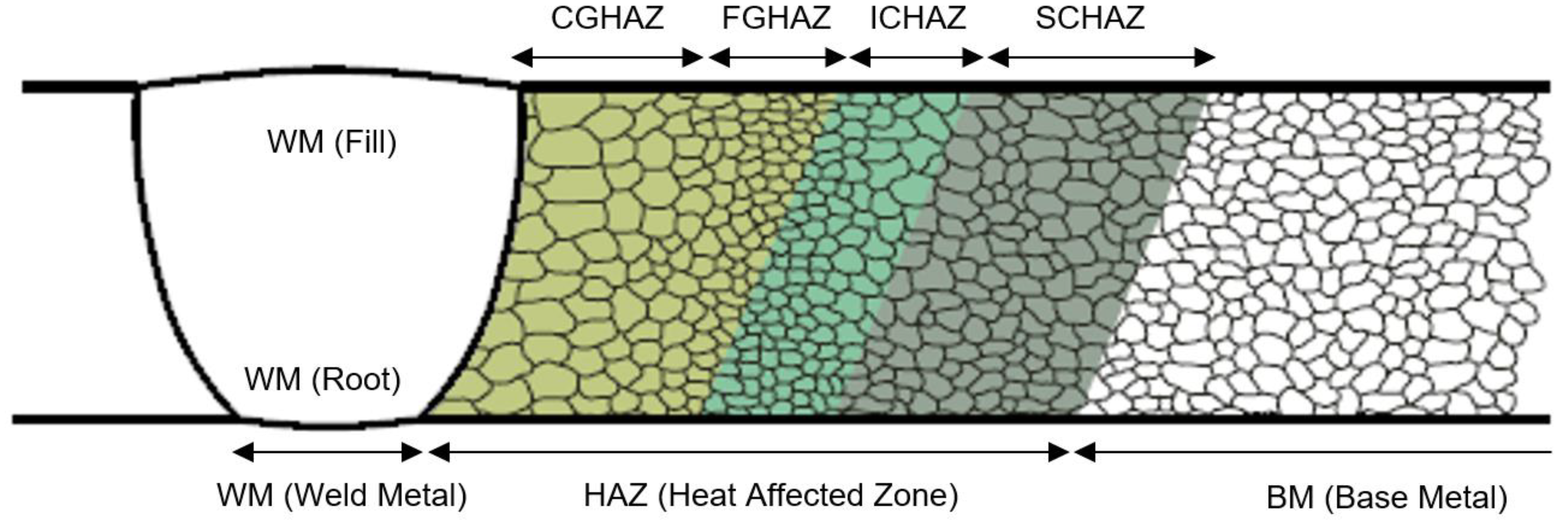
| HAZ Zone | Temperature Range | Mechanical Properties |
|---|---|---|
| CGHAZ | Tγδ < T < Tm | Low toughness, high strength |
| FGHAZ | Ac3 < T < Tγδ | Adequate toughness and strength |
| ICHAZ | Ac1 < T < Ac3 | High toughness, low strength |
| SCHAZ | Ac1 < T | High toughness, low strength |
| Material | Location | Rp0.2 | Rm | A5 | ISO-V 2 | M |
|---|---|---|---|---|---|---|
| [MPa] | [MPa] | [%] | [J] | |||
| S690QL1 1 | BM | 787 | 841 | 22 | 108 (−60 °C) | 1 |
| Mn3Ni1CrMo | WM | 800 | 900 | 19 | 190 (20 °C) | 1.16 (OM) |
| Material | C | Si | Mn | Ni | Cr | Mo | Cu | Al | V | P | S | CEV 1 | CET 2 |
|---|---|---|---|---|---|---|---|---|---|---|---|---|---|
| Chemical Element [% by Weight] | |||||||||||||
| S690QL1 | 0.17 | 0.25 | 1.20 | 0.05 | 0.33 | 0.21 | 0.03 | 0.075 | 0.01 | 0.011 | 0.001 | 0.49 | 0.33 |
| Mn3Ni1CrMo | 0.10 | 0.53 | 1.60 | 1.40 | 0.32 | 0.269 | 0.02 | 0.005 | 0.075 | 0.012 | 0.006 | 0.59 | 0.34 |
| Pass No. | Location | I | U | vw | η | Q | Δt8/5 |
|---|---|---|---|---|---|---|---|
| [A] | [V] | [cm/min] | [kJ/mm] | [s] | |||
| 1–3 | Root | 195 | 26 | 28.5 | 0.8 | 0.85 | 4.4 |
| 4–22 | Fill + Cover | 280 | 29 | 45 | 0.8 | 0.87 | 4.5 |
| MTS Specimen | Location | Welded Joint Zone | MTS Specimen | Location | Welded Joint Zone |
|---|---|---|---|---|---|
| R1–R6 | Fill + Cover | BM | C1–C5 | Root | BM |
| R7–R13 | Fill + Cover | HAZ | C6–C8 | Root | HAZ |
| R14–R25 | Fill + Cover | WM | C9–C10 | Root | WM |
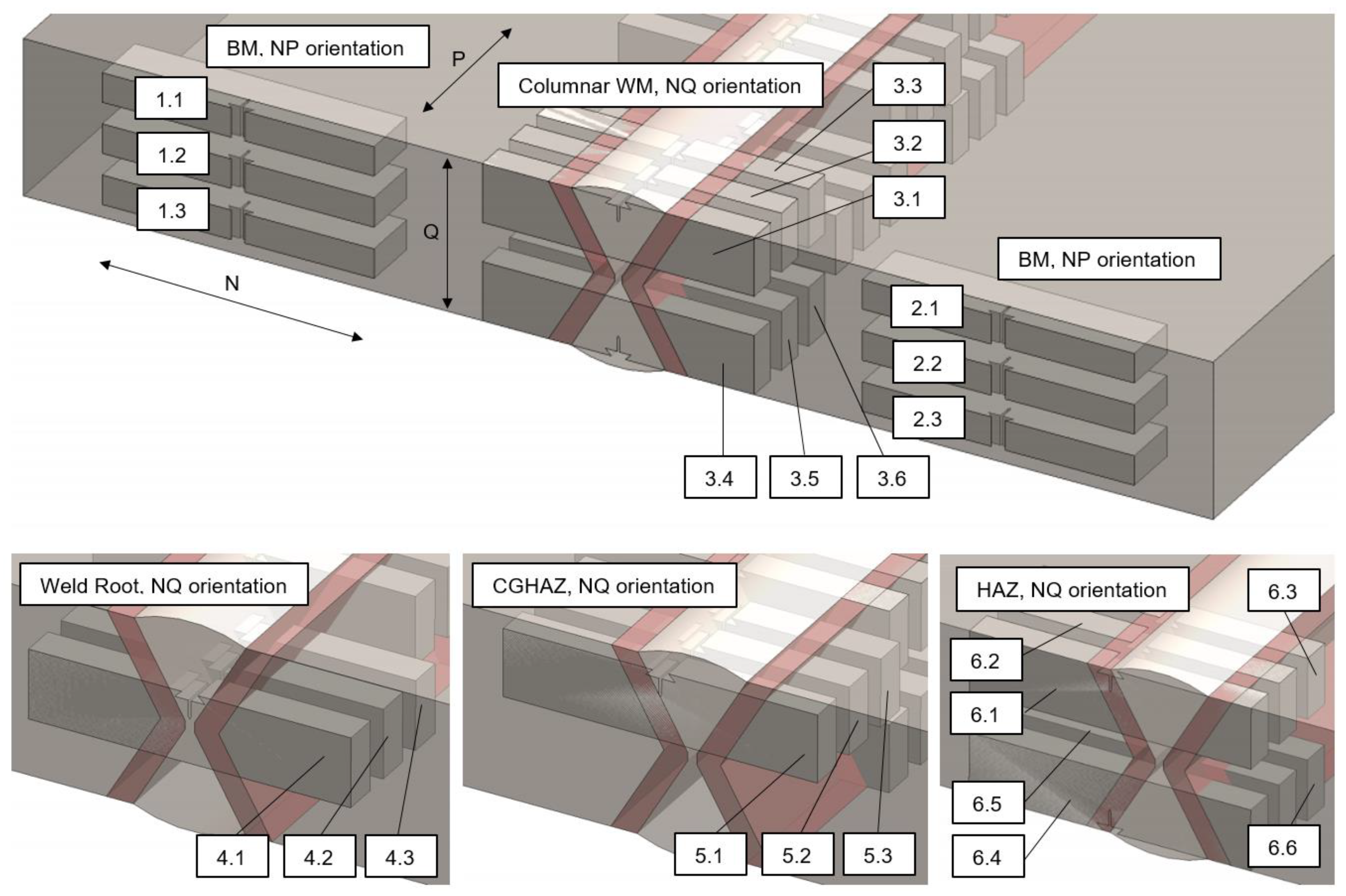
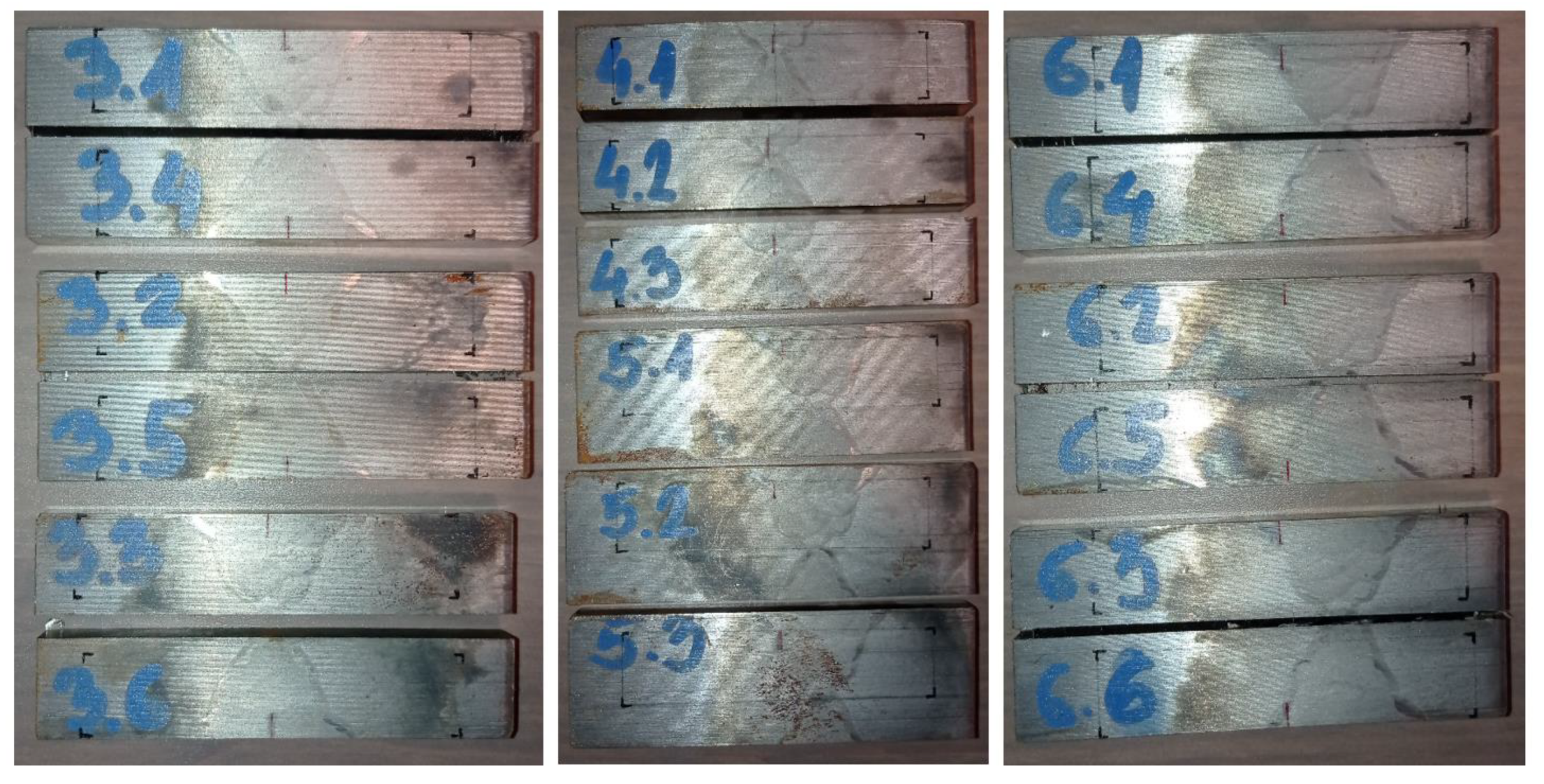
| SENB Specimen | Welded Joint Zone | Orientation | Crack |
|---|---|---|---|
| 1.1–1.3 | BM | NP | Crack initiation and through BM |
| 2.1–2.3 | BM | NP | Crack initiation and through BM |
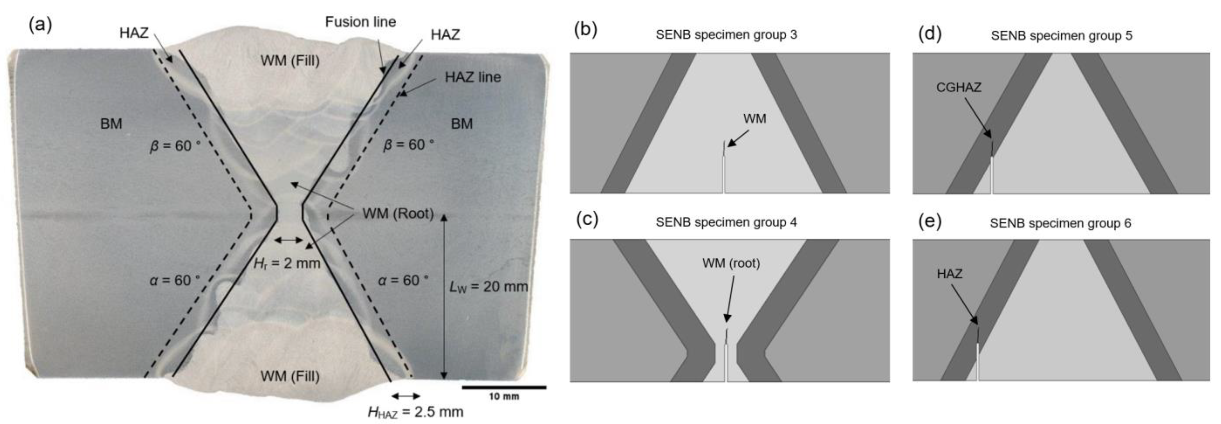
| 3.1–3.6 | WM (Fill) | NQ | Crack initiation and through columnar WM, weld centre line, upper + lower side |
| 4.1–4.3 | WM (Root) | NQ | Crack in WM root, lower side propagation |
| 5.1–5.3 | CGHAZ | NQ | Crack initiation in CGHAZ, adjacent to WM |
| 6.1–6.6 | HAZ | NQ | Crack initiation in HAZ, upper + lower side |
| SENB Specimen | Location | a0 | a0/W | ap | ap/W | Δa |
|---|---|---|---|---|---|---|
| [mm] | [-] | [mm] | [-] | [mm] | ||
| 1.1 | BM | 7.162 | 0.478 | 7.666 | 0.512 | 0.504 |
| 1.2 | BM | 6.791 | 0.454 | 7.240 | 0.484 | 0.449 |
| 1.3 | BM | 6.824 | 0.456 | 7.405 | 0.495 | 0.581 |
| 2.1 | BM | 7.020 | 0.468 | 7.499 | 0.500 | 0.479 |
| 2.2 | BM | 6.679 | 0.446 | 7.312 | 0.488 | 0.633 |
| 2.3 | BM | 6.815 | 0.455 | 7.195 | 0.481 | 0.380 |
| 3.1 | WM (Fill) | 6.001 | 0.400 | 6.693 | 0.446 | 0.692 |
| 3.2 | WM (Fill) | 5.421 | 0.362 | 6.541 | 0.437 | 1.120 |
| 3.3 | WM (Fill) | 5.685 | 0.380 | 6.340 | 0.424 | 0.655 |
| 3.4 | WM (Fill) | 5.665 | 0.378 | 6.564 | 0.438 | 0.899 |
| 3.5 | WM (Fill) | 4.976 | 0.332 | 5.765 | 0.385 | 0.789 |
| 3.6 | WM (Fill) | 5.213 | 0.348 | 5.861 | 0.392 | 0.648 |
| 4.1 | WM (Root) | 5.941 | 0.396 | 6.387 | 0.426 | 0.445 |
| 4.2 | WM (Root) | 5.595 | 0.374 | 6.311 | 0.422 | 0.716 |
| 4.3 | WM (Root) | 5.295 | 0.354 | 5.985 | 0.400 | 0.691 |
| 5.1 | CGHAZ | 7.072 | 0.471 | 7.844 | 0.523 | 0.772 |
| 5.2 | CGHAZ | 6.396 | 0.427 | 6.955 | 0.465 | 0.559 |
| 5.3 | CGHAZ | 5.703 | 0.381 | 6.185 | 0.413 | 0.483 |
| 6.1 | HAZ | 6.060 | 0.404 | 6.549 | 0.437 | 0.489 |
| 6.2 | HAZ | 5.931 | 0.396 | 6.529 | 0.436 | 0.599 |
| 6.3 | HAZ | 4.292 | 0.293 | 4.819 | 0.328 | 0.527 |
| 6.4 | HAZ | 4.907 | 0.328 | 5.489 | 0.367 | 0.583 |
| 6.5 | HAZ | 3.793 | 0.253 | 4.349 | 0.291 | 0.556 |
| 6.6 | HAZ | 3.753 | 0.251 | 5.260 | 0.351 | 1.507 |
| Specimen | Material | E | Rp0.2 | Rm | Δa | CMOD | ||
|---|---|---|---|---|---|---|---|---|
| [GPa] | [MPa] | [MPa] | [mm] | [mm] | [mm] | |||
| SENB DD1 | BM | 210 | 755 | 840 | 0.075 | 0.030 | 1.502 | 0.915 |
| SENB DD2 | BM | 210 | 755 | 840 | 0.075 | 0.055 | 0.495 | 1.008 |
| SENB DD3 | BM/WM | 210/210 | 755/780 | 840/890 | 0.075/0.110 | 0.030/0.055 | 4.561 | 1.009 |
| SENB DD4 | BM/WM | 210/210 | 690/780 | 770/890 | 0.090/0.110 | 0.025/0.200 | 1.722 | 1.004 |
| Specimen | Location | Rp0.2 | Rm | E | Agt |
|---|---|---|---|---|---|
| [MPa] | [MPa] | [GPa] | [%] | ||
| MTS R1 | BM | 739 | 801 | 169.94 | 7.3 |
| MTS R2 | BM | 733 | 805 | 148.84 | 8.1 |
| MTS R3 | BM | 740 | 826 | 137.98 | 6.1 |
| MTS R4 | BM | 737 | 845 | 131.31 | 6.3 |
| MTS R5 | BM | 726 | 827 | 148.39 | 6.9 |
| MTS R6 | BM | 729 | 828 | 164.30 | 7.1 |
| MTS R7 | HAZ | 755 | 838 | 169.10 | 7.2 |
| MTS R8 | HAZ | 755 | 842 | 188.26 | 7.3 |
| MTS R9 | HAZ | 726 | 813 | 193.22 | 6.2 |
| MTS R10 | HAZ | 750 | 842 | 161.03 | 5.5 |
| MTS R11 | HAZ | 891 | 962 | 191.49 | 2.8 |
| MTS R12 | HAZ | 725 | 825 | - | - |
| MTS R13 | HAZ | 875 | 937 | 221.51 | 4.3 |
| MTS R14 | WM | 813 | 849 | 186.16 | 4.9 |
| MTS R15 | WM | 812 | 851 | 180.00 | 6.4 |
| MTS R16 | WM | 844 | 894 | 218.40 | 8.2 |
| MTS R17 | WM | 797 | 874 | 216.09 | 8.2 |
| MTS R18 | WM | 770 | 866 | 176.20 | 6.8 |
| MTS R19 | WM | 797 | 894 | 174.51 | 8.0 |
| MTS R20 | WM | 751 | 846 | 176.07 | 7.9 |
| MTS R21 | WM | 790 | 893 | 200.73 | 7.9 |
| MTS R22 | WM | 763 | 851 | 186.36 | 8.8 |
| MTS R23 | WM | 753 | 842 | 185.10 | 9.0 |
| MTS R24 | WM | 754 | 844 | 213.36 | 8.9 |
| MTS R25 | WM | 761 | 883 | 199.68 | 8.8 |
| Specimen | Location | Rp0.2 | Rm | E | Agt |
|---|---|---|---|---|---|
| [MPa] | [MPa] | [GPa] | [%] | ||
| MTS C1 | BM | 784 | 883 | 165.71 | 5.6 |
| MTS C2 | BM | 793 | 875 | 180.17 | 5.1 |
| MTS C3 | BM | 789 | 861 | 181.72 | 5.0 |
| MTS C4 | BM | 729 | 804 | 171.69 | 5.4 |
| MTS C5 | BM | 764 | 839 | 168.02 | 4.2 |
| MTS C6 | HAZ | 900 | 946 | 179.62 | 4.6 |
| MTS C7 | HAZ | 908 | 977 | 174.44 | 3.4 |
| MTS C8 | HAZ | 854 | 890 | 179.71 | 6.5 |
| MTS C9 | WM | 801 | 848 | 168.20 | 7.2 |
| MTS C10 | WM | 795 | 848 | 180.37 | 7.1 |
| SENB Specimen | Welded Joint Zone | Pmax | CMODmax |
|---|---|---|---|
| [kN] | [mm] | ||
| 1.1–1.3 | BM | 9.40; 8.89; 9.34 | 1.31; 1.02; 1.07 |
| 2.1–2.3 | BM | 9.85; 9.25; 9.38 | 0.75; 1.39; 0.92 |
| 3.1–3.6 | WM (Fill) | 11.98; 11.90; 11.70; 10.48; 12.34; 12.00 | 0.78; 0.82; 0.72; 0.74; 0.56; 0.60 |
| 4.1–4.3 | WM (Root) | 12.02; 12.34; 12.91 | 0.60; 0.81; 0.75 |
| 5.1.-5.3 | CGHAZ | 9.43; 9.89; 11.49 | 1.39; 1.17; 0.99 |
| 6.1–6.6 | HAZ | 11.92; 11.14; 15.59; 14.65; 17.50; 16.51 | 1.24; 1.38; 0.95; 1.25; 0.89; 1.04 |
| SENB Specimen | Welded Joint Zone | JQ(1)/JIC | KJIC | δQ(1)/δIC |
|---|---|---|---|---|
| [kJ/m2] | [MPa∙m1/2] | [mm] | ||
| 1.1–1.3 | BM | 585.00 *; 371.00; 368.00 | 332.22; 264.57; 263.49 | 0.393; 0.263; 0.263 |
| 2.1–2.3 | BM | 278.00; 399.00; 300.50 | 229.02; 274.37; 238.11 | 0.193; 0.285; 0.263 |
| 3.1–3.6 | WM (Fill) | 233.70; 158.00; 241.00; 134.50; 120.00; 165.00 | 215.23; 176.97; 218.56; 163.28; 154.23; 180.85 | 0.165; 0.115; 0.173; 0.097; 0.090; 0.120 |
| 4.1–4.3 | WM (Root) | 185.10; 215.60; 167.30 | 191.54; 206.72; 182.10 | 0.131; 0.152; 0.119 |
| 5.1–5.3 | CGHAZ | 385.60; 440.00; 419.60 | 275.95; 294.77; 287.86 | 0.243; 0.294; 0.262 |
| 6.1–6.6 | HAZ | 629.70; 577.00; 536.00; 680.00; 532.00; 182.00 | 352.56; 337.48; 325.27; 366.37; 324.05; 189.54 | 0.386; 0.360; 0.366; 0.450; 0.370; 0.127 |
| Specimen | Material | E | Rp0.2 | Rm | ||
|---|---|---|---|---|---|---|
| [GPa] | [MPa] | [MPa] | [mm] | |||
| 1.3 | BM | 210 | 735 | 820 | 0.119 | 0.054 |
| 3.6 | BM | 210 | 735 | 820 | 0.119 | 0.054 |
| WM (Fill) | 210 | 780 | 865 | 0.146 | 0.024 | |
| WM (Root) | 210 | 800 | 850 | 0.134 | 0.032 | |
| CGHAZ | 210 | 860 | 925 | 0.078 | 0.038 | |
| HAZ | 210 | 745 | 830 | 0.123 | 0.044 | |
| 4.3 | BM | 210 | 735 | 820 | 0.119 | 0.054 |
| WM (Fill) | 210 | 780 | 865 | 0.149 | 0.028 | |
| WM (Root) | 210 | 800 | 850 | 0.139 | 0.033 | |
| CGHAZ | 210 | 860 | 925 | 0.078 | 0.038 | |
| HAZ | 210 | 745 | 830 | 0.123 | 0.044 | |
| 5.2 | BM | 210 | 735 | 820 | 0.162 | 0.068 |
| WM (Fill) | 210 | 780 | 865 | 0.149 | 0.028 | |
| WM (Root) | 210 | 800 | 850 | 0.139 | 0.033 | |
| CGHAZ | 210 | 860 | 925 | 0.128 | 0.029 | |
| HAZ | 210 | 745 | 855 | 0.164 | 0.073 | |
| 6.3 | BM | 210 | 735 | 820 | 0.162 | 0.068 |
| WM (Fill) | 210 | 780 | 865 | 0.149 | 0.028 | |
| WM (Root) | 210 | 800 | 850 | 0.139 | 0.033 | |
| CGHAZ | 210 | 860 | 925 | 0.128 | 0.029 | |
| HAZ | 210 | 745 | 855 | 0.177 | 0.087 |
| Specimen | Material | Δa(EXP) | Δa(NUM) | Δa(diff.) | CMOD(EXP) | CMOD(NUM) | CMOD(diff.) |
|---|---|---|---|---|---|---|---|
| [mm] | [mm] | [%] | [mm] | [mm] | [%] | ||
| 1.3 | BM | 0.581 | 0.583 | 0.34 | 1.070 | 1.083 | 1.21 |
| 3.6 | WM (Fill) | 0.648 | 0.659 | 1.68 | 0.600 | 0.609 | 1.49 |
| 4.3 | WM (Root) | 0.691 | 0.697 | 0.86 | 0.750 | 0.761 | 1.46 |
| 5.2 | CGHAZ | 0.559 | 0.577 | 3.17 | 1.170 | 1.172 | 0.17 |
| 6.3 | HAZ | 0.527 | 0.527 | 0 | 0.950 | 0.955 | 0.52 |
Disclaimer/Publisher’s Note: The statements, opinions and data contained in all publications are solely those of the individual author(s) and contributor(s) and not of MDPI and/or the editor(s). MDPI and/or the editor(s) disclaim responsibility for any injury to people or property resulting from any ideas, methods, instructions or products referred to in the content. |
© 2023 by the authors. Licensee MDPI, Basel, Switzerland. This article is an open access article distributed under the terms and conditions of the Creative Commons Attribution (CC BY) license (https://creativecommons.org/licenses/by/4.0/).
Share and Cite
Tomerlin, D.; Kozak, D.; Ferlič, L.; Gubeljak, N. Experimental and Numerical Analysis of Fracture Mechanics Behavior of Heterogeneous Zones in S690QL1 Grade High Strength Steel (HSS) Welded Joint. Materials 2023, 16, 6929. https://doi.org/10.3390/ma16216929
Tomerlin D, Kozak D, Ferlič L, Gubeljak N. Experimental and Numerical Analysis of Fracture Mechanics Behavior of Heterogeneous Zones in S690QL1 Grade High Strength Steel (HSS) Welded Joint. Materials. 2023; 16(21):6929. https://doi.org/10.3390/ma16216929
Chicago/Turabian StyleTomerlin, Damir, Dražan Kozak, Luka Ferlič, and Nenad Gubeljak. 2023. "Experimental and Numerical Analysis of Fracture Mechanics Behavior of Heterogeneous Zones in S690QL1 Grade High Strength Steel (HSS) Welded Joint" Materials 16, no. 21: 6929. https://doi.org/10.3390/ma16216929
APA StyleTomerlin, D., Kozak, D., Ferlič, L., & Gubeljak, N. (2023). Experimental and Numerical Analysis of Fracture Mechanics Behavior of Heterogeneous Zones in S690QL1 Grade High Strength Steel (HSS) Welded Joint. Materials, 16(21), 6929. https://doi.org/10.3390/ma16216929