Abstract
In order to facilitate the prediction of some physical properties, we propose several simple formulas based on two parameters only, the metallic valence and metallic atomic radii. Knowing the composition, for single-phase alloys, the average parameters can be calculated by the rule of mixture. The input parameters can be obtained from tabulated databases. Adopting from the literature the results of Coulomb crystal model for metals and single-phase high-entropy alloys, we have derived formulas for the shear modulus (G) and the cohesion energy (Ecoh). Based on these parameters separately, we set up two formulas to estimate the hardness in the case of pure metals. For single-phase (solid-solution) HEAs, by simplifying the Maresca and Curtin model, we obtained a formula for estimating the hardness, which takes into account the atomic misfit in addition to G. The maximal hardness for single-phase HEA is approximately 600 kg/mm2 and is obtained for a composition with a valence electron concentration of approximately 6 ÷ 7.
1. Introduction
The process of designing materials from the first principles is not usually a straight-forward or simple one. It requires large computer capacities and selection between the competing models [1]. Machine learning [2], as a branch of artificial intelligence, can help overcome the shortcomings of long-term experiments and computational simulations and effectively shorten the design of new alloys. However, we lack a deeper understanding of cause and effect relationships. This is why simple phenomenological connections are more effective and reveal the physical content as well.
The physical properties of alloys are defined at the atomic level. This is why one is tempted to work with semi-empirical models based on atomic valences and bond distances. Such papers have been published on volumetric lattice energy [3,4], bond ionicity [5] and the melting point [6].
In order to facilitate the design of high-entropy alloys (HEAs), a simple approximate electrostatic model is presented using only the atomic valences and atomic radii. In this model, a metal can be considered as a “one-component plasma” (OCP) [7], which is a system of positive point charge embedded in a uniform distributed compensating negative charge sea of valence electrons. The OCP model is very popular nowadays because it can be applied in different systems like charge-stabilized colloids [8] and dense neutron stars [9,10].
When the ratio, Γ, of electrostatic energy to thermal energy, exceeds a value of Γ = 175, OCP freezes into a body-centered cubic (bcc) Coulomb crystal, which can be treated classically [7]. It was shown in the literature [10,11,12] that the matter in the cores of white dwarfs and the crusts of neutron stars can be modeled as a Coulomb crystal of fully pressure-ionized atomic nuclei with a nearly incompressible background of strongly degenerate electrons. We suppose that the elastic properties of their matter can be treated as similar to those of metals where the exchange interaction of the electrons is neglected as a first approximation in the calculation of the shear modulus. This is the basic supposition of the present work.
It is worth mentioning that in 1962, Keyes [13] presented a conjecture concerning the electrostatic origin of the elastic moduli. Based on dimensional analysis, he proposed a normalization factor, which is equal to the electrostatic energy per unit volume: e2/R4, where e is the electric charge and R is the atomic radius. Based on the electrostatic origin of the shear (and also of bulk) modulus, a formula for the shear modulus, G, can be simply derived as the second derivative of electrostatic energy. J. Gilman obtained, by a “back-on -the envelope” calculation [14], the following estimation formula.
where e is the charge of the electron and R is the atomic radius.
Formula (1), however, is a rough approximation because the valence of the metal is not taken into account.
The aim of this work is to use the results published in the literature [10,11,12] on the Coulomb crystal to calculate the shear modulus, G, and then, based on own considerations, to extend the Coulomb crystal model calculations to the cohesion energy, Ecoh, of single-phase metal alloys (pure metals and high-entropy alloys). Then, we set up two formulas to estimate the hardness based on G and Ecoh and compare the goodness of the estimation. The formulas are tested first on pure metals and then it is applied for HEAs compositions. In the case of multicomponent single-phase HEAs, solid-solution hardening will be discussed in addition to the result obtained by the rule of mixture applied to the component elements.
2. New Approaches on Estimation of Physical Properties
2.1. Prediction of the Shear Modulus
Modelling the metal with a Coulomb crystal, we a going to calculate the shear moduli (and later the cohesive energy) applying a severe simplification based on the “equivalent (or effective) atom” [11]. This can be performed for an isotropic alloy where all of the atoms in the Coulomb crystal are the same. The calculations are based on electrostatics determining the potential energy of the equivalent atom. This equivalent atom is actually a positive nucleus immersed in a uniform electron cloud of mean square radius, Rm.
For such a Coulomb lattice, the elastic constants were calculated by Baiko [10,11], and using the Voight, Reuss and Hill approximations [12], the effective shear modulus G is given [12] as:
where is the number density with two atoms/cell, and a is the length of the side of the cubic cell containing two atoms, nN is the number density of atoms, Z is the valence number of the positive ions, Rws is the Wigner–Seitz atomic radius and e is the elementary charge. Formula (2) should be multiplied with 9 × 10⁹ In order to get the result in SI units, and the Wigner–Seitz radius replaced by atomic metallic radius for BCC system Rm = 0.8793 × Rws.
Inserting the numerical factors after some algebra, we obtain a formula which depends on two tabulated properties only, the valence Z and the metallic atomic radius, Rm, which are easily accessible at [15]:
where Rm is in Å and Z is the valence and the unit for Geff is GPa.
It is the basic observation of this paper that Formula (2) calculated for neutron stars is equally valid for the polycrystalline metals—just the number density must be matched to the condensed matter data and the value of Z is not the proton number of ionic nuclei (which has lost all its electrons) but the number of valence electrons given in the common electron sea background. The exact number of valence electrons depends on the property under calculations. For chemical reactions and corrosion behavior, the chemical valence should be applied (in general the sum of the electrons on the last s-p shell); for the cohesion energy, however, where the bonding character should be accentuated, in addition to the outer shell sp electrons, the uncompensated d electrons must be taken into consideration. We considered that the valence of Miedema, ZBM, calculated from the bulk modulus, B, is the most appropriate to calculate the shear modulus. Miedema valences were calculated from the tabulated data of B and Vm using the following equation [16]:
where the molar volume, Vm (cm3), is calculated from the atomic mass (A) and density ρ (Vm = A/ρ) and the atomic volume .
It should be mentioned that the valence Z is used as the valence electron number per atom (e/a), the contribution of each atom to the shared electron sea and should be distinguished from the valence electron count (VEC), which comprises the electrons on the outer electron shells (s-p-d), a part of them, participates only conditionally in the metallic bond.
The Rm and Z data of the elements used in practice according to the three most common crystal lattice symmetries are collected in Table 1, together with the calculated shear modulus values using Formula (3).

Table 1.
The calculated shear modulus and cohesion energy using Equations (3) and (8) and comparison with the tabulated values.
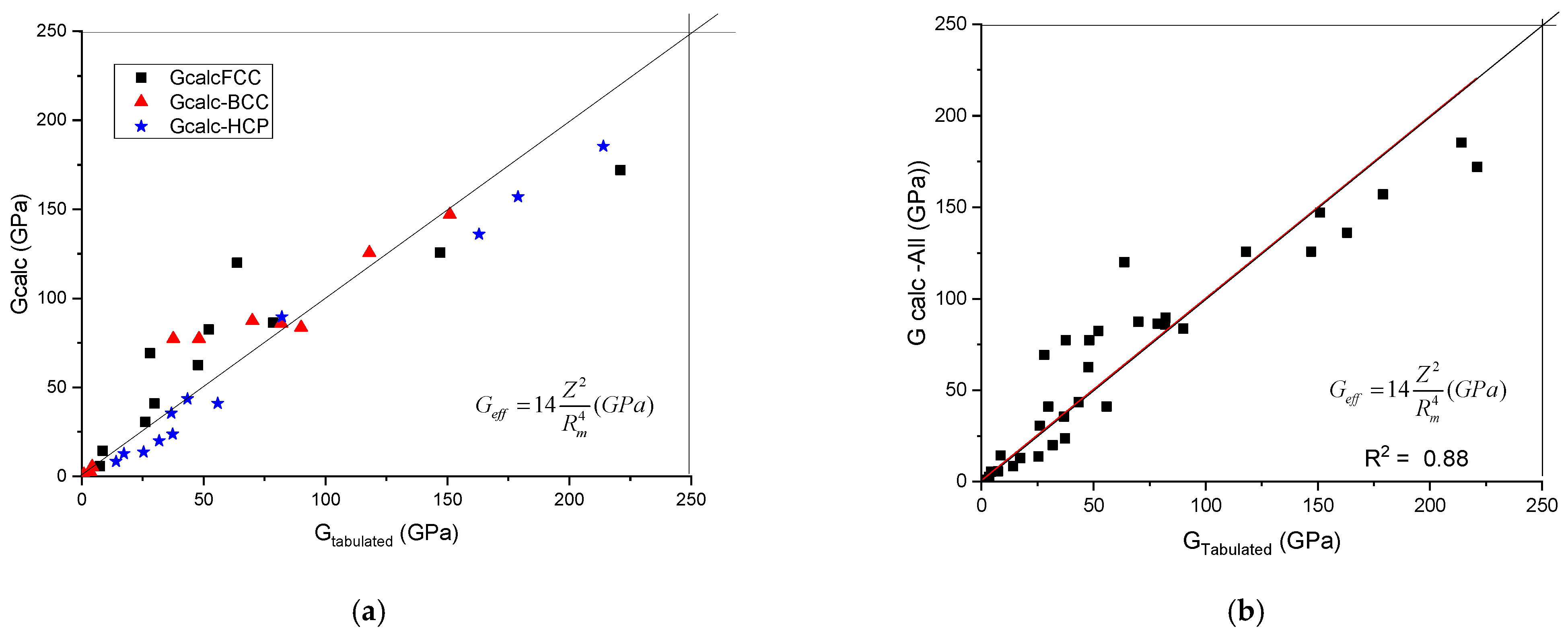
The calculated shear modulus, Gcalc, as a function of tabulated ones is presented in Figure 1. It can be seen that the data line up along the first angle bisector. No separation of the data as a function of crystalline structure was found. To establish the quality of the goodness of fit, we treated the data belonging to the three crystal symmetries together (see Figure 1b) and a R2 value of 0.88 was obtained.
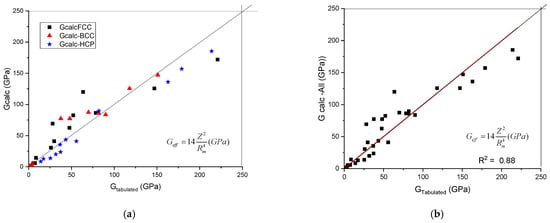
Figure 1.
A plot of the calculated shear modulus against the tabulated (accepted) values. (a) distinguished according to crystal structure, (b) plotted together to establish the goodness of fit.
2.2. Estimation of the Cohesion Energy
We have adopted a simple metal model, which is composed of positive ionic cores distributed in a regular crystallographic lattice and the negative sea of valence electrons. The Coulombian interaction takes place between the cation with a charge +Ze and the partial number of surrounding electrons, –e/n. Taking a coordination number of 12, attractive interaction will be manifested between 6 ion pairs only at a given moment:
where d is the distance between the atoms in Angstrom, d = 2Rm, Rm is the metallic atomic radius in Å, and then the unit of the cohesion energy is eV.
Md is the Madelung constant summing up the effect of surrounding atoms. Its value is approximately 1.716 [17], and it was used to calculate the numerical factor in Formula (6).
For comparison, let us recall the formulas valid for ionic binding [17]:
where Md = 1.716 is the Madelung number and d is the distance between the atoms in Angstrom.
We find differences in two points. First, for metals, the binding energy is proportional to the valence, whereas for ionic binding to the product of valences; and second, for metals, the Madelung number is divided by 6, because from 12 near neighbors, only 6 pairs can be formed and, at a given moment, only 1/6 parts of interactions is effective. Although the higher valence somewhat compensates for this 1/6 multiplier, in general, the metallic bond is weaker than the ionic one.
It is to be observed that the cohesion energy formula does not contain free parameters for fitting the results. Certainly, these formulas are only approximate. The calculated data of Equation (6) are systematically 15–20% greater than the accepted ones. The reason for this is presumably that the influence of the environment was taken into account in an unsatisfactory way, that is, the Madelung constant must be reduced by a factor of 0.82. Finally, the formula recommended for alloy design is:
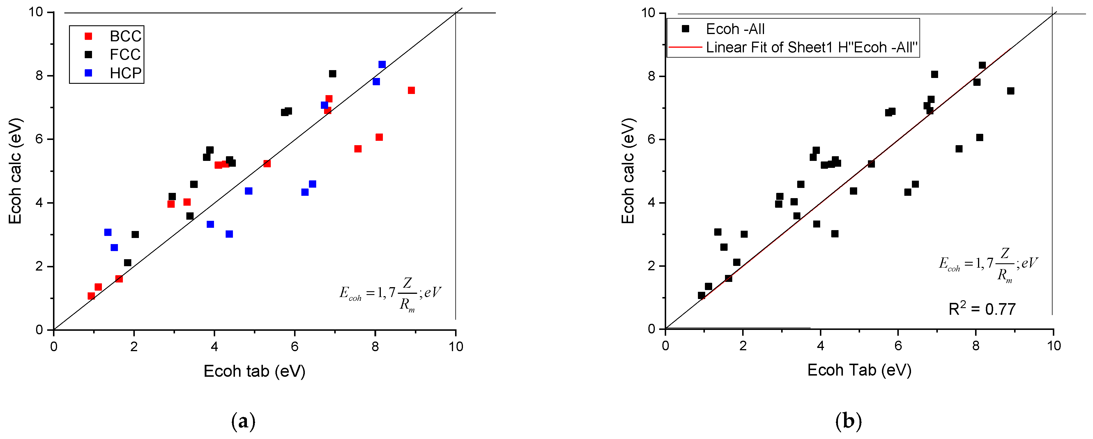
Using the Z and Rm data collected in Table 1, the calculated cohesion energies as a function of tabulated ones are shown in Figure 2. It can be seen that the data points line up along the first angle bisector, with an R2 = 0.77. No separation of the data as a function of crystalline structure can be observed.
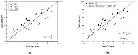
Figure 2.
A plot of the calculated cohesion energy against the tabulated ones. (a) distinguished according to crystal structure, (b) plotted together to establish the goodness of fit.
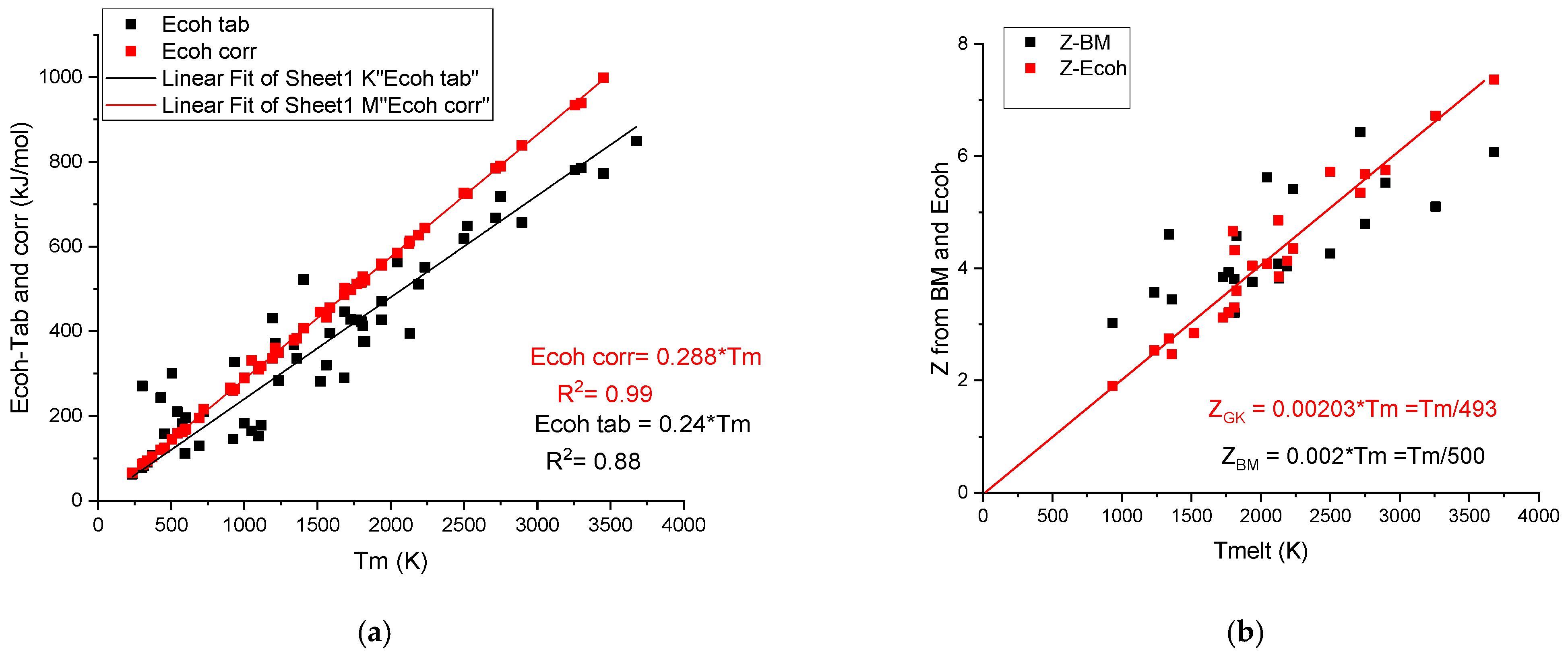
It is worth mentioning that there is a strong correlation between the cohesion energy and the melting temperature:
Figure 3a shows a strong correlation with R2 = 0.88 between the tabulated values and Tm. G. Kaptay [18] applied a correction to the tabulated cohesion energy data, obtaining a perfect linear correlation:
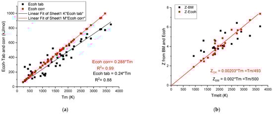
Figure 3.
(a) The linear corrected (GK) and scattered uncorrected (Tab) cohesion energy data versus melting temperature. The difference increases with the increasing melting temperature. (b) The calculated valences Z-Bm and Z-Ecoh values versus melting temperature.
The corrected values of cohesion energies, Ecoh-corr, are as an average 0.288/0.24 = 1.18-fold larger than the average uncorrected (tabulated) values. This correction beneficially increases the accuracy of the prediction when we estimate hardness using cohesive energy.
It is worth noting that based on Equation (8) of the cohesion energy, an effective valency can be determined, which is also a linear function of the melting temperature. Valences, ZGK, determined using the corrected cohesion energies [18], are less scattering (see Figure 3b) around the fitting line (ZGK = 0.00203*Tm) than the valences determined based on bulk modulus, ZBM, using the Miedema model (Equation (4)). The average Z is approximately Tm/500 in both cases (see Table 2). The large metallic valence number, Z, for transition metal elements shows that in addition to the s-p electrons, the d electrons participate also in the common valence electron sea. As to our knowledge, the above presented correlation between the metallic valence and the melting temperature was not yet discussed in the literature.
Table 2.
Comparison of the valences determined from Equations (5) and (8).
2.3. Estimation of HV from the Cohesion Energy, Ecoh
In order to predict and tailor the hardness of single-phase HEAs we need a prior relationship, with calculable or measurable parameters. We first examine how to derive hardness from cohesive energy and then from elastic moduli.
Based on dimensional analyses, we suggest that the HV is proportional to the cohesion energy multiplied with the electron density, n = Z/Vm, where Z is the metallic valence and Vm is the molar volume. In this way, in addition to the unpaired d electrons, the sp electrons are taken into account as well in determining of hardness. The phenomenological equation is:
where C is a constant to be determined, Z is the valence, Ec is in kJ/mol (1 eV/atom = 96.485 kJ/mol) and Vm is in cm3, then the unit of the calculated hardness, HV calc., is in GPa.
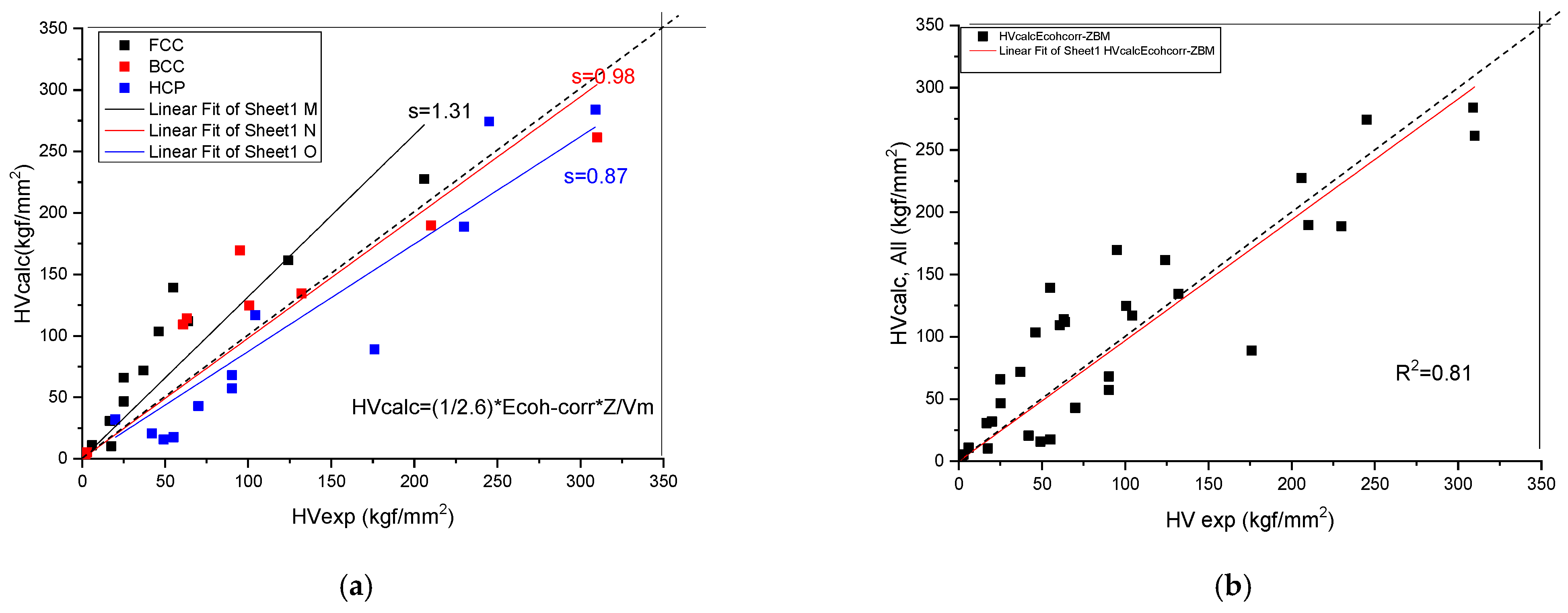
We have found (see Figure 4 and Table 3) a rather good correlation between the calculated and measured values although the measured hardness values published in the literature [19] show a great range. Unfortunately, the tabulated Ec and Z values show a great range also. This is why it is necessary for a review article to collect and comment on the valence and atomic radii data published in the literature so far.
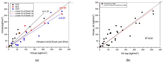
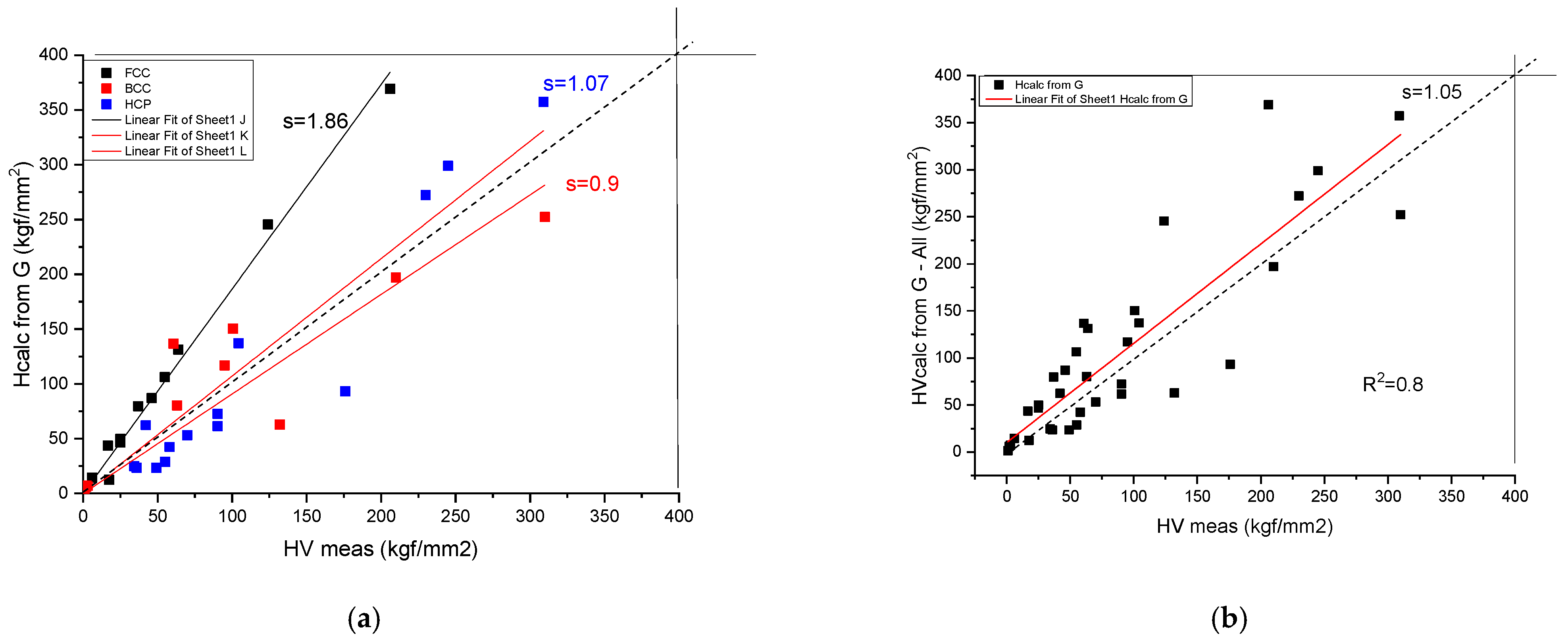
Figure 4.
Correlation of the measured and calculated Vickers Hardness based on Formula (9) for pure metals. (a) distinguished according to crystal structure, (b) plotted together to establish the goodness of fit.
Table 3.
Calculation of HV for pure elements from G and Ecoh.
A normalizing factor C = 1/(100*2.6) adjusts the values to GPa and finally the dimensions to the measured values is obtained by multiplying by 100, because 1 GPa = 100 kgf/mm2. For high-entropy alloys, all three parameters (Ec, Z and Vm) can be calculated as a weighted average of the elemental values. Equation (9) permits estimation of the low bound for hardness of any single-phase alloy.
Formula (9) is a good addition to the literature [19], where various correlations between hardness and different elastic moduli or a combination of them have been published. However, the best correlation can be achieved with the shear modulus, G, which can be understood by the creation and movement of the dislocation, which is not facilitated by the volume change, but by the shear deformation.
2.4. Estimation of Hardness, HV, from the Shear Modulus, G
It was shown [19] that for brittle alloys (BMG and compounds), where the plastic deformation is negligible compared to the elastic one, there is a direct relationship between HV and G:
For pure metals and ductile HEAs, however, an order of magnitude greater calculated hardness results from Equation (10). This is why a new relationship is necessary to calculate the hardness based on elastic moduli. We start from the formula given in the literature [20]:
where we change E to G and apply the well-known relations valid for isotropic materials and and we obtain the hardness as a function of G and of Pugh [21] (ductile–brittle) parameter, G/B. Not that a sample is ductile for G/B < 0.6, and brittle for G/B > 0.6.
For a representative value of G/B = 3/8, the result is:
which matches the order of magnitude of the experimental HV values. For more exact matching, a fitting coefficient, C, is determined (see Figure 5):
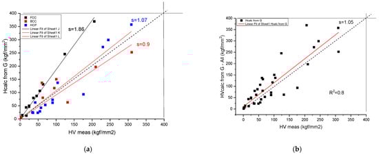
Figure 5.
Correlation of the measured and calculated Vickers Hardness based on Formula (14) for pure metals. (a) distinguished according to crystal structure, (b) plotted together to establish the goodness of fit.
2.5. Estimation of Hardness of Single-Phase HEAs
The basic parameters, the atomic radii and valences, will be calculated using the rule of mixture (ROM), where the weighted average is calculated against the concentration of the elements, as
In order to estimate the hardness of single-phase HEAs, we need a new parameter, the atomic size misfit, which is the mean squared deviation of the atomic size, Ra or Rws:
We have to distinguish between volume per atom, Vws = Vm/NA, and atomic volume, Va, where from the corresponding Wigner–Seitz, Rws and atomic, Ra, radii can be determined. It should be emphasized that whereas Rws is independent of crystalline structure, the Ra depends on the structure because the atomic radii is defined as half of the distance between the atoms. The relations between the Ra and the lattice constant, a, for the relevant three crystalline structures of the single-phase HEAs are the following: Ra = a*√3/4 for BCC, Ra = a*√2/4 for FCC and Ra = a/2 for HCP. The volume per unit cell is a3 for BCC and FCC and c*a3*3√3/2 for HCP structures, while the number of atoms per unit cell is 2 for BCC, 4 for FCC and 6 for HCP structures, respectively. Performing simple calculations, we find Ra = 0.8793*Rws for BCC, Ra = 0.9046 * Rws for FCC and Ra = 0.9117 * Rws for HCP structures.
The expression of atomic size as Ra and Rws is important when one calculates the atomic misfit δa and δws. These two misfit parameters are the same when the alloy and all the constituents belong to the same crystalline structure. In a number of cases, however, there are constituents with different structures like the HCP Ti-Zr-Hf elements in BCC refractory alloys or the FCC Al in BCC transition metal alloys. In such a case, we have to recalculate the Ra parameter of the element from the structure-insensitive Rws using the above formulas and then we will obtain the same misfit parameters, δa = δws. For example, for HCP titanium, we have from the tabulated data: Rws = 1.6145 Å and Ra = 1.4707 Å. In BCC alloy, we have to consider Ra = 1.635 Å (and a = 3.27 Å) for calculation of the atomic misfit.
The shear modulus <G> and the cohesion energy <Ecoh> will be calculated with ROM and with the Equations (3) and (8), respectively, using the weighted averaged R and Z values from Equation (16). The match of the data is acceptable. However, the calculated hardness values from G (Equation (15)) and from Ecoh (Equation (9)) are approximately 3–4-smaller than the measured ones (see Table 4). It is considered that this discrepancy can be attributed mainly to solid-solution hardening (SSH) as the other possible contributions like the grain boundary, second phase and precipitation strengthening will be neglected for the as-cast alloy samples.
SSH originates from lattice distortion, which is characterized by the atomic misfit due to the different elements in the multicomponent HEAs. A number of papers are dealing with numerical calculations of the yield stress (YS) and of the Vickers Hardness (HV = 3*YS) of solid-solution hardened alloys [22,23,24]. However, the scaling factor and the ratio of edge and screw dislocations are rather arbitrarily estimated, although the atomic misfit and elastic modulus misfit are accurately calculated. Therefore, we dare to make a reasonable simplification in the equations published in the literature for predicting the hardness due to solid-solution hardening.
Starting from Varennes’s concepts [22], Maresca and Curtin [24] developed a model applying the material constants available from the literature. They obtained the yield stress contribution of solid-solution hardening (SSH) as:
where “G” and “ν” are the isotropic alloy elastic constants (shear modulus and Poison constant) and “b” is the alloy Burgers vector, calculated using Vegard’s law to determine the alloy volume (b = (4 V)1/3/(1/2)0.5). The computed misfit volumes closely follow Vegard’s law, ΔVi = Vi − <V>, where <V> = ΣciVi is the alloy atomic volume and Vi the elemental BCC atomic volumes. “α” is the line tension parameter, α = 1/12.
The term containing the Poisson factor varies between 1.5 and 3. Let us take the most representative value of 2.5, and then the numerical factors can be simplified to
The sum in parenthesis can be written as , where δw is the atomic size misfit expressed in terms of atomic radii.
Finally, we arrived to a formula which contains two parameters of the HEA, the averaged shear modulus, G, and the atomic misfit:
The hardness increase due to solid-solution hardening can be estimated as
HV = 3σy.
The predicted hardness will be quantified as the sum of two contributions: the starting hardness of constituents calculated with the rule of mixture:
and the contribution from solid-solution hardening given by Equation (22):
HVbase = ΣciHVi
Creating a database from the literature, it turns out that for the majority of cases, HVbase = 60 ± 20 and the fitted value for proportionality constant, K = 0.7, as long as the unit of G is in GPa.
As a result of all these approximations, the calculated value for the hardness of single- phase HEAs is:
In Table 4, a number of 106 HEAs were selected from the literature and the predicted hardness (Equation (24)) is compared to the measured one in Figure 6. We tried to find experimental hardness data that apply to single-phase alloys.
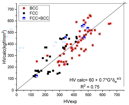
Figure 6.
Comparison of the calculated and measured hardness values for BCC- and FCC-type HEAs.
The goodness of fit, R2 = 0.74, is acceptable considering the scattering of the measured HV data and the number of approximations to express the formula for solid-solution hardening. Perusing Table 3, one can observe that no alloy sample with a shear modulus larger than 100 can be found. The atomic mismatch factor, δw, should be smaller than 6.5% for single-phase structures [25]. Applying Equation (24), we obtain HV = 900 kgf/mm2 as a theoretical upper limit for the hardness of HEA alloys.
Interestingly, serious deviation from the measured HV values, requiring addition of a much larger constant (150 ÷ 200 instead 60) signals the presence of precipitation hardening, and the alloy can no longer be considered as a single-phase material.
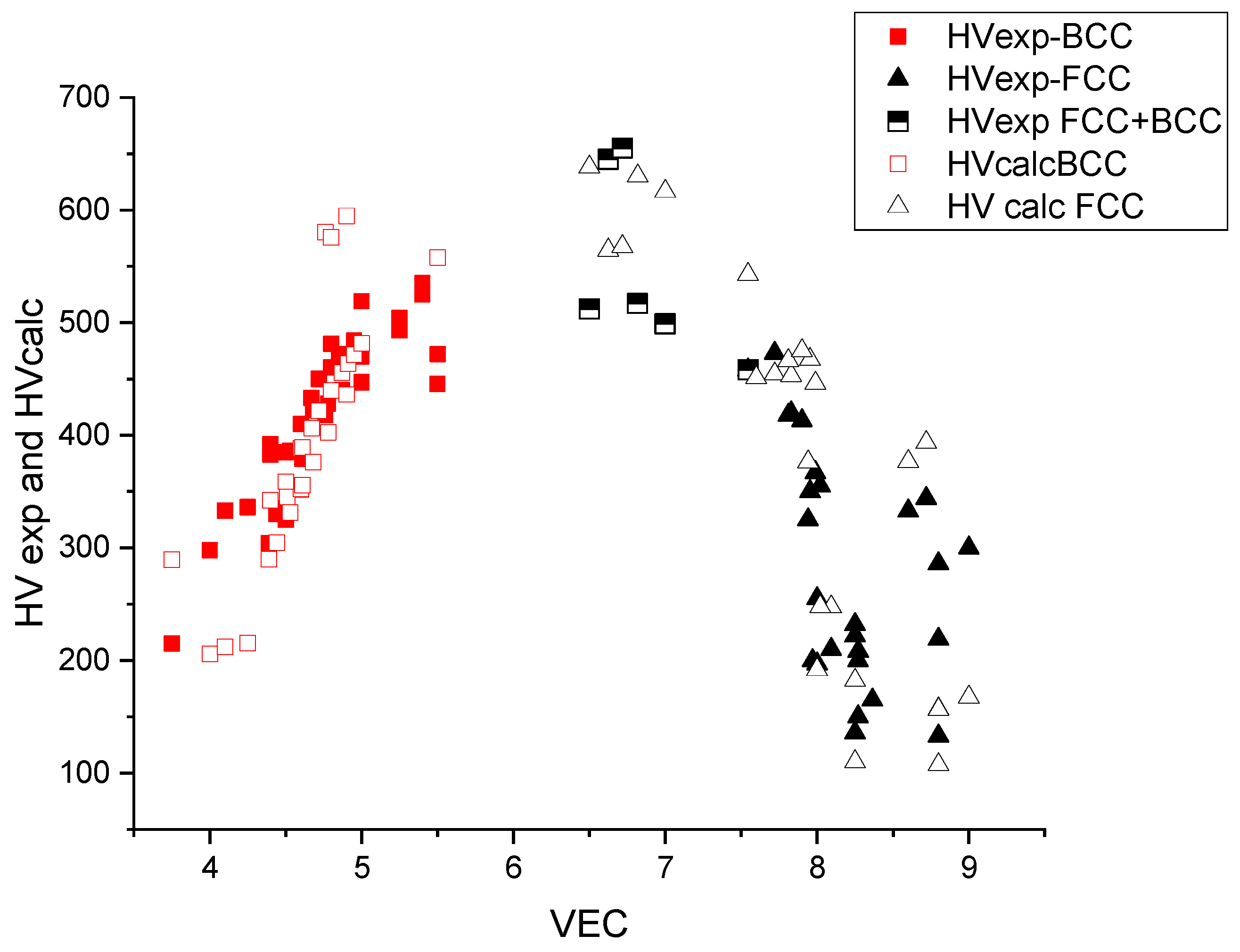
In Figure 7, the measured and calculated HV data are represented as a function of VEC. The maximum is approximately VEC = 6–7, which corresponds to the maximal, d = VEC − 2 = 5, uncompensated d electrons and hence to the maximal bonding strength (see Friedel model in [26,27]). The maximal hardness is approximately 600 kgf/mm2 and decreases both around VEC = 4 (refractory HEAs) and VEC = 8 (derivatives of FCC Cantor alloy).
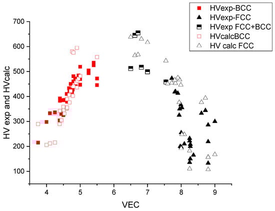
Figure 7.
The hardness versus the average valence electronic concentration (VEC) for BCC- and FCC-type HEAs.
From Figure 7, we can see that for small values of VEC, the structure is BCC and for large values, FCC. The structure is no longer single phase for intermediate VEC values. The extent of this double-phase (BCC + FCC) region is between 7.5 and 7.8, according to [28,29]. This double-phase region coincides with the maximum of the hardness as a function of VEC, which makes it difficult to interpret the hardness values in terms of solid-solution hardening only. The lack of BCC data around VEC = 6.5 is due to the fact that alloying the element of column 6 (Cr, Mo, W) with Fe and Co results in precipitation of intermetallic compounds like sigma phase [28] and it is difficult to find real single-phase HEAs with VEC = 6.5 in the literature.
Table 4.
Comparison of calculated (Equation (24)) and experimental hardnesses of more than 100 single-phase high-entropy alloys.
Table 4.
Comparison of calculated (Equation (24)) and experimental hardnesses of more than 100 single-phase high-entropy alloys.
| Alloy | VEC | HVexp (kgf/mm2) | Gave (GPa) | δw (%) | HVcalc (kgf/mm2) BCC | HVcalc (kgf/mm2) FCC | HC calc (kgf/mm2) BCC + FCC | Ref. | |
|---|---|---|---|---|---|---|---|---|---|
| Nb28.3Ti24.5V23Zr24.2 | BCC | 4.51 | 335 | 39.4 | 5.92 | 355.3 | -- | -- | [30] |
| Nb22.6Ti19.4V37.2Zr20.8 | BCC | 4.60 | 352 | 40.4 | 6.43 | 398.1 | -- | -- | [30] |
| Cr24.6Nb26.7Ti23.9Zr24.8 | BCC | 4.76 | 418 | 50.6 | 7.61 | 590.1 | -- | -- | [30] |
| Cr20.2Nb20Ti19.9V19.6Zr20.3 | BCC | 4.80 | 481 | 50.35 | 7.59 | 585.7 | -- | -- | [30] |
| Y25Ti25Zr25Hf25 | BCC | 3.75 | 215 | 22.99 | 7.58 | 299.6 | -- | -- | pw |
| Ti33.33Zr33.33Hf33.34 | BCC | 4.00 | 298 | 35.01 | 4.00 | 215.6 | -- | -- | pw |
| Ti30Zr30Hf30Nb10 | BCC | 4.10 | 333 | 35.27 | 4.10 | 222.0 | -- | -- | pw |
| Ti25Zr25Hf25Nb25 | BCC | 4.25 | 336 | 35.67 | 4.13 | 225.4 | -- | -- | pw |
| Ti20Zr20Hf20Nb20V20 | BCC | 4.40 | 392 | 37.32 | 6.12 | 352.4 | -- | -- | pw |
| Ti25Zr25V25Nb25 | BCC | 4.50 | 385 | 39.57 | 6.10 | 368.7 | -- | -- | pw |
| Ti20Zr20V20Nb20Ta20 | BCC | 4.60 | 410 | 45.01 | 5.45 | 362.2 | -- | -- | pw |
| V25Nb25Mo25W25 | BCC | 5.50 | 472 | 89.88 | 3.06 | 339.5 | -- | -- | pw |
| TiZrNbV | BCC | 4.50 | 325 | 39.57 | 6.10 | 368.7 | -- | -- | [31] |
| TiZrNbVMo0.3 | BCC | 4.61 | 379 | 44.14 | 6.03 | 399.1 | -- | -- | [31] |
| TiZrNbVMo0.5 | BCC | 4.67 | 433 | 46.9 | 5.98 | 416.3 | -- | -- | [31] |
| TiZrNbVMo0.7 | BCC | 4.72 | 450 | 49.46 | 5.93 | 431.6 | -- | -- | [31] |
| TiZrNbVMo1.0 | BCC | 4.80 | 460 | 52.95 | 5.84 | 449.8 | -- | -- | [31] |
| TiZrNbVMo1.3. | BCC | 4.87 | 440 | 56.1 | 5.76 | 465.4 | -- | -- | [31] |
| TiZrNbVMo1.5 | BCC | 4.91 | 472 | 58.02 | 5.70 | 473.5 | -- | -- | [31] |
| TiZrNbVMo1.7 | BCC | 4.95 | 484 | 59.83 | 5.65 | 481.4 | -- | -- | [31] |
| TiZrNbVMo2.0 | BCC | 5.00 | 519 | 62.28 | 5.58 | 491.5 | -- | -- | [31] |
| TiZrNbV0.3 | BCC | 4.39 | 304 | 38.42 | 5.16 | 299.8 | -- | -- | [31] |
| TiZrNbV0.3Mo0.1 | BCC | 4.44 | 330 | 40.28 | 5.21 | 314.7 | -- | -- | [31] |
| TiZrNbV0.3Mo0.3 | BCC | 4.53 | 386 | 43.74 | 5.28 | 341.5 | -- | -- | [31] |
| TiZrNbV0.3Mo0.5 | BCC | 4.61 | 383 | 46.89 | 5.33 | 365.6 | -- | -- | [31] |
| TiZrNbV0.3Mo0.7 | BCC | 4.68 | 422 | 49.78 | 5.35 | 386.0 | -- | -- | [31] |
| TiZrNbV0.Mo1.03 | BCC | 4.78 | 428 | 53.69 | 5.36 | 412.5 | -- | -- | [31] |
| TiZrNbV0.3Mo1.5 | BCC | 4.90 | 464 | 59.27 | 5.33 | 446.3 | -- | -- | [31] |
| NbCrMo0.5Ta0,5TiZr | BCC | 4.90 | 469 | 58.34 | 6.98 | 604.7 | -- | -- | [31] |
| NbTiVZr | BCC | 4.50 | 335 | 39.57 | 6.10 | 368.7 | -- | -- | [23] |
| AlCoCrFeNi | BCC | 7.20 | 478.2 | 71.2 | 5.28 | 518.2 | -- | -- | [32] |
| AlCoCrFeNi | BCC | 7.20 | 509.6 | 71.2 | 5.28 | 518.2 | -- | -- | [33] |
| AlCoCrFeNi | BCC | 7.20 | 523.7 | 71.2 | 5.28 | 518.2 | -- | -- | [34] |
| AlCoCrFeNiV0.2 | BCC | 7.03 | 546.8 | 70.1 | 5.36 | 520.2 | -- | -- | [34] |
| AlCoCrFeNiV0.5 | BCC | 6.99 | 579.9 | 68.79 | 5.14 | 487.6 | -- | -- | [34] |
| AlCoFeNi | BCC | 7.50 | 441 | 60.69 | 5.88 | 510.8 | -- | -- | [35] |
| Al18Co20Cr21Fe20Ni21 | BCC | 7.30 | 497.8 | 72.9 | 5.10 | 508.4 | -- | -- | [36] |
| Al0.3HfNbTaTiZr | BCC | 4.30 | 345.9 | 40.63 | 4.12 | 247.8 | -- | -- | [37] |
| Al0.75HfNbTaTiZr | BCC | 4.21 | 141.5 | 39.65 | 4.23 | 249.7 | -- | -- | [37] |
| Al0.25MoNbTiV | BCC | 4.97 | 450.9 | 57.03 | 4.51 | 357.5 | -- | -- | [38] |
| HfMo0.25NbTaTiZr | BCC | 4.47 | 387.1 | 44.96 | 4.27 | 278.0 | -- | -- | [39] |
| HfMoTaTiZr | BCC | 4.60 | 531.5 | 53.92 | 5.08 | 389.6 | -- | -- | [40] |
| HfNbTaTiZr | BCC | 4.40 | 328.3 | 41.36 | 4.01 | 244.4 | -- | -- | [39] |
| HfNbTaTiZr | BCC | 4.40 | 289.1 | 41.36 | 4.01 | 244.4 | -- | -- | [41] |
| NbTaTiV | BCC | 4.75 | 311.3 | 49.1 | 3.57 | 247.5 | -- | -- | [42] |
| NbTaTiVW | BCC | 5.00 | 438 | 70.4 | 3.30 | 302.1 | -- | -- | [42] |
| NbTaVW | BCC | 5.25 | 483 | 77.5 | 3.54 | 352.7 | -- | -- | [42] |
| Hf0.5Nb0.5Ta0.5Ti1.5Zr | BCC | 4.25 | 295 | 40.71 | 4.18 | 251.9 | -- | -- | [43] |
| NbTiZr | BCC | 4.33 | 289.1 | 37.82 | 4.27 | 243.4 | -- | -- | [41] |
| FeCrNiCoAl2 | BCC | 6.50 | 512 | 66.66 | 6.69 | 648.2 | -- | -- | [29] |
| FeCrNiCoAl1.5 | BCC | 6.82 | 517 | 70.36 | 6.36 | 640.3 | -- | -- | [29] |
| FeCrNiCOAl1.25 | BCC | 7.00 | 499 | 72.47 | 6.11 | 626.6 | -- | -- | [29] |
| fecrnicocual3 | BCC | 6.63 | 645 | 59.25 | 6.61 | 574.5 | -- | -- | [29] |
| fecrnicocual2.8 | BCC | 6.72 | 655 | 60.1 | 6.57 | 577.6 | -- | -- | [29] |
| FeCrNiCoAl2 | BCC | 6.50 | 512 | 66.66 | 6.69 | 648.2 | -- | -- | [29] |
| FeCrNiCoAl1.5 | BCC | 6.82 | 517 | 70.36 | 6.36 | 640.3 | -- | -- | [29] |
| FeCrNiCOAl1.25 | BCC | 7.00 | 499 | 72.47 | 6.11 | 626.6 | -- | -- | [29] |
| -- | -- | -- | -- | -- | -- | -- | -- | -- | |
| CoCrFeMnNi | FCC | 8.00 | 132.3 | 84.72 | 1.58 | 169.1 | -- | [44] | |
| CoCrFeNi | FCC | 8.25 | 131.5 | 87.59 | 1.13 | 132.2 | -- | [45] | |
| CoCrFeNiTi0.5 | FCC | 7.77 | 497.2 | 80.5 | 4.96 | 536.6 | -- | [46] | |
| CoFeNi | FCC | 8.99 | 119.5 | 77.7 | 1.11 | 122.5 | -- | [35] | |
| CoFeNiV | FCC | 8.00 | 233.5 | 68.7 | 3.25 | 291.5 | -- | [47] | |
| Al5Co35Fe20Ni35Ti5 | FCC | 8.60 | 313.9 | 70.94 | 4.63 | 443.2 | -- | [48] | |
| Co10Cr10Fe40Mn40 | FCC | 7.50 | 140.1 | 81.4 | 1.08 | 123.1 | -- | [49] | |
| Co5(CrFeMnNi)95 | FCC | 7.81 | 150.9 | 86.43 | 1.51 | 164.8 | -- | [50] | |
| Co10(CrFeMnNi)90 | FCC | 7.88 | 144.1 | 85.86 | 1.54 | 166.9 | -- | [50] | |
| Co20(CrFeMnNi)80 | FCC | 8.00 | 149.9 | 84.72 | 1.58 | 169.1 | -- | [50] | |
| CoCrFeMnNi | FCC | 8.00 | 172.6 | 84.72 | 1.58 | 169.1 | -- | [51] | |
| CoCrFeNi | FCC | 8.25 | 156.9 | 87.59 | 1.43 | 158.8 | -- | [45] | |
| Co0.5CrFeNi1.5Ti0.3 | FCC | 8.07 | 303.8 | 83.19 | 4.14 | 447.1 | -- | [52] | |
| CoCu0.5FeNiTa0.1 | FCC | 9.16 | 183.6 | 73.05 | 2.97 | 278.3 | -- | [53] | |
| CrFeNi2Ti0.3 | FCC | 8.18 | 328.3 | 83.31 | 4.16 | 450.2 | -- | [52] | |
| -- | -- | -- | -- | -- | -- | -- | -- | -- | |
| FeCrNiCoAlCu0,5 | F + B | 7.55 | 458 | 72.36 | 5.51 | 552.9 | [54] | ||
| FeCrNiCoCu | FCC | 8.80 | 133 | 79.2 | 1.03 | 117.7 | -- | [54] | |
| FeCrNiCoTi0.3 | FCC | 7.95 | 350 | 84 | 4.35 | 477.5 | -- | [55] | |
| FeCrNiCo | FCC | 8.25 | 136 | 87 | 0.99 | 120.1 | -- | [55] | |
| FeCrNiCoMo0.3 | FCC | 8.09 | 210 | 89.3 | 2.37 | 257.5 | -- | [54] | |
| FeCrNiCoCu | FCC | 8.80 | 133 | 79.2 | 1.03 | 117.7 | -- | [54] | |
| -- | -- | -- | -- | -- | -- | -- | -- | -- | |
| FeNiCrCuCo | FCC | 8.80 | 286 | 79.47 | 1.35 | 143.3 | -- | [54] | |
| AlCo0.5CrCuFeNi | F + B | 7.72 | 473 | 66.9 | 4.94 | 454.0 | [56] | ||
| CoCrFeNi-Pd1.5 | FCC | 8.72 | 344 | 73.4 | 3.96 | 381.9 | -- | [56] | |
| CoCrFeNi-Pd | FCC | 8.60 | 333 | 77 | 3.64 | 361.8 | -- | [56] | |
| CoCrFeNiCu | FCC | 8.80 | 219 | 79.4 | 1.35 | 142.9 | -- | [56] | |
| Al0.5CoCrCuFeNi | FCC | 8.27 | 208 | 72.74 | 3.88 | 370.4 | -- | [56] | |
| CoCrCuFeNiAl0.5 | FCC | 8.27 | 200 | 72.74 | 3.88 | 370.4 | -- | [56] | |
| CoCrFeNi | FCC | 8.25 | 232 | 87.59 | 1.43 | 158.8 | -- | [55] | |
| CoCrFeNi | FCC | 8.25 | 222 | 87.5 | 1.43 | 158.7 | -- | [45] | |
| CoCrNiCu | FCC | 9.00 | 300 | 78.8 | 1.45 | 150.5 | -- | [55] | |
| FeNiCrCuAl | F + B | 7.60 | 342 | 66.2 | 4.99 | 455.1 | [55] | ||
| AlCoCr0.5CuFeNi | FCC | 7.99 | 367 | 63.3 | 5.07 | 445.9 | -- | [54] | |
| AlCoCrCuFeNi | FCC | 7.83 | 420 | 67.5 | 4.86 | 449.0 | -- | [56] | |
| CoCrFeNi-Mn | FCC | 8.00 | 255 | 84.7 | 1.58 | 169.1 | -- | [56] | |
| CoCrFeNi-V0.3 | FCC | 8.02 | 355 | 84.2 | 2.17 | 225.6 | -- | [54] | |
| CoCrFeNiCuAl0.5V0.6 | FCC | 7.94 | 325 | 69.85 | 3.98 | 368.4 | -- | [54] | |
| AlCoCrCuFe0.5Ni | FCC | 7.81 | 418 | 66.27 | 5.05 | 461.9 | -- | [54] | |
| Co64Cr30W5C1 | FCC | 7.90 | 413 | 93.13 | 3.60 | 419.7 | -- | [57] | |
| -- | -- | -- | -- | -- | -- | -- | -- | -- | |
| Co10Cr10Fe40Mn40 | F + B | 7.50 | 140.1 | 81.4 | 1.08 | 123.1 | [49] | ||
| Co5(CrFeMnNi)95 | FCC | 7.81 | 150.9 | 86.43 | 1.51 | 164.8 | -- | [50] | |
| Co10(CrFeMnNi)90 | FCC | 7.88 | 144.1 | 85.86 | 1.54 | 166.9 | -- | [50] | |
| Co20(CrFeMnNi)80 | FCC | 8.00 | 149.9 | 84.72 | 1.58 | 169.1 | -- | [50] | |
| -- | -- | -- | -- | -- | -- | -- | -- | -- | - |
| Al0.2CoCrFeNiTi0.5 | FCC | 7.57 | 469.8 | 77.45 | 5.33 | 564.7 | [46] | ||
| CoCrFeMnNi | FCC | 8.00 | 132.3 | 84.72 | 1.52 | 169.1 | -- | [58] | |
| CoCrFeNi | FCC | 8.25 | 131.5 | 87.59 | 1.43 | 132.2 | -- | [45] | |
| CoCrFeNiTi0.5 | FCC | 7.77 | 497.2 | 80.58 | 4.96 | 536.6 | [46] | ||
| CoFeNi | FCC | 8.99 | 119.5 | -- | -- | 122.5 | -- | [35] | |
| CoFeNiV | FCC | 8.00 | 233.5 | -- | -- | 291.5 | -- | [47] |
3. Conclusions
- The metallic material was treated as a one-component plasma, where the positive ions with a charge equal to the metallic valence are embedded in the negative see of valence electrons. The results of coulomb crystal calculations concerning the shear modulus of neutron stars were adopted from the literature for metallic alloys.
- The effective shear modulus can be calculated using only two parameters, valence, Z, and atomic radius, Rm(Å), as:
- A formula for the cohesion energy was obtained using purely electrostatic considerations as a function of only two parameters, valence Z, and atomic radius Rm(Å), as:
This formula permitted a new estimation of metallic valences based on the cohesion energy. Based on the strong correlation between the cohesion energy and the melting temperature, a simple formula can be derived for metallic valence:
Z = Tm/500
- 4.
- We present formulas to estimate the hardness of pure elements from Ec and G:where [HVcalc] = kgf/mm2, [G] = GPa, [Ec]= kJ/mol, [Rm] = Å, and [Vm] = cm3.
A slight dependence on crystal structure was found in both cases.
- 5.
- Applying a number of simplifications and approximations to the solid-state strengthening formula of Maresca and Curtin, a simple formula was obtained to calculate the hardness of single-phase HEAs:where [HVcalc] = kgf/mm2 and [G] = GPa.
Author Contributions
Conceptualization, L.K.V.; Validation, L.V.; Investigation, L.K.V.; Data curation, O.K.T.; Writing—original draft, L.K.V.; Writing—review & editing, O.K.T., N.Q.C. and L.V.; Visualization, O.K.T.; Supervision, N.Q.C. All authors have read and agreed to the published version of the manuscript.
Funding
This research was funded by Hungarian Scientific Research Fund OTKA, Grant numbers: 128229.
Institutional Review Board Statement
Not applicable.
Informed Consent Statement
Not applicable.
Data Availability Statement
The original contributions presented in the study are included in the article, further inquiries can be directed to the corresponding author.
Conflicts of Interest
Author Ottó K. Temesi is employed by the H-ion Ltd. Company and the SMARTUS Zrt. Company. The remaining authors declare that the research was conducted in the absence of any commercial or financial relationships that could be construed as a potential conflict of interest.
References
- Vitos, L. Computational Quantum Mechanics for Materials Engineers: The EMTO Method and Applications; Springer: Berlin/Heidelberg, Germany, 2007. [Google Scholar]
- Liu, X.; Zhang, J.; Pei, Z. Machine learning for high-entropy alloys: Progress, challenges and opportunities. Prog. Mater. Sci. 2023, 131, 101018. [Google Scholar] [CrossRef]
- Plendl, J.N.; Gielisse, P.J. Hardness of Nonmetallic Solids on an Atomic Basis. Phys. Rev. 1962, 125, 828–832. [Google Scholar] [CrossRef]
- Grimvall, G.; Thiessen, M. Science of Hard Materials. In Proceedings of the International Conference on the Science of Hard Materials 1984; Institute of Physics Conference Series Number 75; Adam Hilger Ltd.: Boston, MA, USA, 1986; p. 61. [Google Scholar]
- Julg, A. An Empirical Relationship between Hardness and Bond Ionicity in Crystals. Phys. Chem. Miner. 1987, 3, 45–53. [Google Scholar] [CrossRef]
- Kisly, P.S. Proceedings of the International Conference on the Science of Hard Materials; Almond, E.A., Brookes, C.A., Warren, R., Eds.; Adam Hilger Ltd.: Bristol, UK; Boston, MA, USA, 1984; p. 107. [Google Scholar]
- Gillan, M.J. A simple model for the classical one-component plasma. J. Phys. C Solid State Phys. 1974, 7, L1. [Google Scholar] [CrossRef]
- Tamashiro, M.N.; Levin, Y.; Barbosa, M.C. Debye-Hückel-Bjerrum theory for charged colloids. Physica A 1998, 258, 341. [Google Scholar] [CrossRef]
- Zerah, G.; Clerouin, J.; Pollock, E.L. Thomas-Fermi Molecular-Dynamics, Linear Screening, and Mean-Field Theories of Plasmas. Phys. Rev. Lett. 1992, 69, 446. [Google Scholar] [CrossRef] [PubMed]
- Baiko, D.A. Shear modulus of neutron star crust. Mon. Not. R. Astron. Soc. 2011, 416, 22–31. [Google Scholar] [CrossRef]
- Baiko, D.A. Shear Modulus of a Coulomb Crystal of Ions: Effects of Ion Motion and Electron Background Polarization. Contrib. Plasma Phys. 2012, 52, 157–160. [Google Scholar] [CrossRef]
- Kobyakov, D.; Pethick, C.J. Elastic properties of polycrystalline dense matter. Mon. Not. R. Astron. Soc. Lett. 2015, 449, L110–L112. [Google Scholar] [CrossRef]
- Keyes, R.W. Elastic Properties of Diamond-Type Semiconductors. J. Appl. Phys. 1962, 33, 3371–3372. [Google Scholar] [CrossRef]
- Gilman, J.J. Electronic Basis of the Strength of Materials; Cambridge University Press: Cambridge, UK, 2003. [Google Scholar]
- Available online: www.knowledgedoor.com (accessed on 24 April 2024).
- Li, C.; Wu, P. Correlation of Bulk Modulus and the Constituent Element Properties of Binary Intermetallic Compounds. Chem. Mater. 2001, 13, 4642–4648. [Google Scholar] [CrossRef]
- Harrison, W. Simple calculation of Madelung constant. Phys. Rev. B 2006, 73, 212103. [Google Scholar] [CrossRef]
- Kaptay, G.; Csicsovszki, G.; Yaghmaee, M.S. An Absolute Scale for the Cohesion Energy of Pure Metals. Mater. Sci. Forum 2003, 414–415, 235–240. [Google Scholar] [CrossRef]
- Chen, X.Q.; Niu, H.; Li, D.; Li, Y. Modeling hardness of polycrystalline materials and bulk metallic glasses. Intermetallics 2011, 19, 1275–1281. [Google Scholar] [CrossRef]
- Miao, N.; Sa, B.; Zhou, J.; Sun, Z. heoretical investigation on the transition metal borides with Ta3B4-type structure: A class of hard and refractory materials. Comput. Mater. Sci. 2011, 50, 1559–1566. [Google Scholar] [CrossRef]
- Pugh, S.F. XCII. Relations between the elastic moduli and the plastic properties of polycrystalline pure metals. Lond. Edinb. Dublin Philos. Mag. J. Sci. 1954, 45, 823–843. [Google Scholar] [CrossRef]
- Varvenne, C.; Leyson, G.P.M.; Ghazisaeidi, M.; Curtin, W.A. Solute strengthening in random alloys. Acta Mater. 2017, 124, 660–683. [Google Scholar] [CrossRef]
- Yao, H.W.; Qiao, J.W.; Hawk, J.A.; Zhou, H.F.; Chen, M.W.; Gao, M.C. Mechanical properties of refractory high-entropy alloys: Experiments and modelling. J. Alloys Compd. 2017, 696, 1139–1150. [Google Scholar] [CrossRef]
- Maresca, F.; Curtin, W.A. Mechanistic origin of high strength in refractory BCC highentropy alloys up to 1900K. Acta Mater. 2020, 182, 235–249. [Google Scholar] [CrossRef]
- Melnick, A.B.; Soolshenko, V.K. Prediction of Stable Composition for High-Entropy Refractory Alloys. Metallofiz. Noveishie Tekhnol. 2016, 38, 1395–1405. [Google Scholar] [CrossRef]
- Temesi, O.; Varga, L.K.; Chinh, N.Q.; Vitos, L. Estimation of hardness of single-phase metallic alloys. In Proceedings of RQ17 Conference, Warsaw, Poland, 20–25 August 2023. [Google Scholar]
- Temesi, O.; Varga, L.K.; Li, X.; Vitos, L.; Chinh, N.Q. Estimation of Shear Modulus and Hardness of High-Entropy Alloys Made from Early Transition Metals Based on Bonding Parameters. Materials 2023, 16, 2311. [Google Scholar] [CrossRef] [PubMed]
- Gorban’, V.F.; Krapivka, N.A.; Firstov, S.A. High-entropy alloys: Interrelations between electron concentration, phase composition, lattice parameter, and properties. Phys. Met. Metallogr. 2017, 118, 970–981. [Google Scholar] [CrossRef]
- Tian, F.; Varga, L.K.; Chen, N.; Shen, J.; Vitos, L. Empirical design of single phase high-entropy alloys with high hardness. Intermetallics 2015, 58, 1–6. [Google Scholar] [CrossRef]
- Senkov, O.N.; Senkova, S.V.; Miracle, D.B.; Woodward, C. Mechanical properties of low-density, refractory multi-principal element alloys of the Cr–Nb–Ti–V–Zr system. Mater. Sci. Eng. A 2013, 565, 51–62. [Google Scholar] [CrossRef]
- Wu, Y.D.; Cai, Y.H.; Chen, X.H.; Wang, T.; Si, J.J.; Wang, L.; Wang, Y.D.; Hui, X.D. Phase composition and solid solution strengthening effect in TiZrNbMoV high-entropy alloys. Mater. Des. 2015, 83, 651–660. [Google Scholar] [CrossRef]
- Cao, L.G.; Wang, X.H.; Wang, Y.M.; Zhang, L.L.; Yang, Y.; Liu, F.B.; Cui, Y. Microstructural evolution, phase formation and mechanical properties of multi-component AlCoCrFeNix alloys. Appl. Phys. A Mater. 2019, 125, 699. [Google Scholar] [CrossRef]
- Ma, S.G.; Zhang, Y. Effect of Nb addition on the microstructure and properties of AlCoCrFeNi high-entropy alloy. Mater. Sci. Eng. A 2012, 532, 480–486. [Google Scholar] [CrossRef]
- Dong, Y.; Zhou, K.; Lu, Y.; Gao, X.; Wang, T.; Li, T. Effect of vanadium addition on the microstructure and properties of AlCoCrFeNi high entropy alloy. Mater. Des. 2014, 57, 67–72. [Google Scholar] [CrossRef]
- Zuo, T.T.; Li, R.B.; Ren, X.J.; Zhang, Y. Effects of Al and Si addition on the structure and properties of CoFeNi equal atomic ratio alloy. J. Magn. Magn. Mater. 2014, 371, 60–68. [Google Scholar] [CrossRef]
- Chen, C.; Pang, S.; Cheng, Y.; Zhang, T. Microstructure and mechanical properties of Al20-xCr20+0.5xFe20Co20Ni20+0.5x high entropy alloys. J. Alloys Compd. 2016, 659, 279–287. [Google Scholar] [CrossRef]
- Lin, C.M.; Juan, C.C.; Chang, C.H.; Tsai, C.W.; Yeh, J.W. Effect of Al addition on mechanical properties and microstructure of refractory AlxHfNbTaTiZr alloys. J. Alloys Compd. 2015, 624, 100–107. [Google Scholar] [CrossRef]
- Chen, S.Y.; Yang, X.; Dahmen, K.A.; Liaw, P.K.; Zhang, Y. Microstructures and Crackling Noise of AlxNbTiMoV High Entropy Alloys. Entropy 2014, 16, 870–884. [Google Scholar] [CrossRef]
- Juan, C.C.; Tseng, K.K.; Hsu, W.L.; Tsai, M.H.; Tsai, C.W.; Lin, C.M.; Chen, S.K.; Lin, S.J.; Yeh, J.W. Solution strengthening of ductile refractory HfMoxNbTaTiZr high-entropy alloys. Mater. Lett. 2016, 175, 284–287. [Google Scholar] [CrossRef]
- Juan, C.C.; Tsai, M.H.; Tsai, C.W.; Lin, C.M.; Wang, W.R.; Yang, C.C.; Chen, S.K.; Lin, S.J.; Yeh, J.W. Enhanced mechanical properties of HfMoTaTiZr and HfMoNbTaTiZr refractory high-entropy alloys. Intermetallics 2015, 62, 76–83. [Google Scholar] [CrossRef]
- Zyka, J.; Malek, J.; Vesely, J.; Lukac, F.; Cizek, J.; Kuriplach, J.; Melikhova, O. Microstructure and Room Temperature Mechanical Properties of Different 3 and 4 Element Medium Entropy Alloys from HfNbTaTiZr System. Entropy 2019, 21, 114. [Google Scholar] [CrossRef] [PubMed]
- Yao, H.W.; Qiao, J.W.; Gao, M.C.; Hawk, J.A.; Ma, S.G.; Zhou, H.F.; Zhang, Y. NbTaV-(Ti,W) refractory high-entropy alloys: Experiments and modeling. Mater. Sci. Eng. A 2016, 674, 203–211. [Google Scholar] [CrossRef]
- Sheikh, S.; Shafeie, S.; Hu, Q.; Ahlstrom, J.; Persson, C.; Vesely, J.; Zyka, J.; Klement, U.; Guo, S. Alloy design for intrinsically ductile refractory high-entropy alloys. J. Appl. Phys. 2016, 120, 164902. [Google Scholar] [CrossRef]
- He, J.Y.; Liu, W.H.; Wang, H.; Wu, Y.; Liu, X.J.; Nieh, T.G.; Lu, Z.P. Effects of Al addition on structural evolution and tensile properties of the FeCoNiCrMn high-entropy alloy system. Acta Mater. 2014, 62, 105–113. [Google Scholar] [CrossRef]
- Salishchev, G.A.; Tikhonovsky, M.A.; Shaysultanov, D.G.; Stepanov, N.D.; Kuznetsov, A.V.; Kolodiy, I.V.; Tortika, A.S.; Senkov, O.N. Effect of Mn and V on structure and mechanical properties of high-entropy alloys based on CoCrFeNi system. J. Alloys Compd. 2014, 591, 11–21. [Google Scholar] [CrossRef]
- Dong, Y.; Lu, Y. Microstructure and Properties of Multi-component AlxCoCrFeNiTi0.5 High-entropy Alloys. Mater. Sci. Forum 2013, 42, 265–275. [Google Scholar] [CrossRef]
- Jiang, L.; Cao, Z.Q.; Jie, J.C.; Zhang, J.J.; Lu, Y.P.; Wang, T.M.; Li, T.J. Effect of Mo and Ni elements on microstructure evolution and mechanical properties of the CoFeNixVMoy high entropy alloys. J. Alloys Compd. 2015, 649, 585–590. [Google Scholar] [CrossRef]
- Bala, P.; Gorecki, K.; Bednarczyk, W.; Watroba, M.; Lech, S.; Katualko, J. Effect of high-temperature exposure on the microstructure and mechanical properties of the Al5Ti5Co35Ni35Fe20 high-entropy alloy. J. Mater. Res. Technol. 2020, 9, 551–559. [Google Scholar] [CrossRef]
- Chen, L.B.; Wei, R.; Tang, K.; Zhang, J.; Jiang, F.; He, L.; Sun, J. Heavy carbon alloyed FCC-structured high entropy alloy with excellent combination of strength and ductility. Mater. Sci. Eng. A 2018, 716, 150–156. [Google Scholar] [CrossRef]
- Zhu, Z.G.; Ma, K.H.; Yang, X.; Shek, C.H. Annealing effect on the phase stability and mechanical properties of (FeNiCrMn)(100-x)Cox high entropy alloys. J. Alloys Compd. 2017, 695, 2945–2950. [Google Scholar] [CrossRef]
- Zhu, Z.G.; Ma, K.H.; Wang, Q.; Shek, C.H. Compositional dependence of phase formation and mechanical properties in three CoCrFeNi-(Mn/Al/Cu) high entropy alloys. Intermetallics 2016, 79, 1–11. [Google Scholar] [CrossRef]
- Shun, T.-T.; Chang, C.-H. The effects of substitution of Co with Ni on microstructure, mechanical properties, and age hardening of Co1-xCrFeNi1+xTi0.3 high-entropy alloys. Mater. Sci. Eng. A 2019, 763, 138181. [Google Scholar] [CrossRef]
- Xu, T.T.; Lu, Y.P.; Cao, Z.Q.; Wang, T.M.; Li, T.J. Effects of Ta Addition on the Microstructure and Mechanical Properties of CoCu0.5FeNi High-Entropy Alloy. J. Mater. Eng. Perform. 2019, 28, 7642–7648. [Google Scholar] [CrossRef]
- Li, C.; Li, J.C.; Zhao, M.; Jiang, Q. Effect of alloying elements on microstructure and properties of multiprincipal elements high-entropy alloys. J. Alloys Compd. 2009, 475, 752–757. [Google Scholar] [CrossRef]
- Sakai, M. The Meyer hardness: A measure for plasticity? J. Mater. Res. 1999, 14, 3630–3639. [Google Scholar] [CrossRef]
- Mizutani, U. Hume-Rothery Rules for Structurally Complex Alloy Phases; CRC Press: Boca Raton, FL, USA, 2011. [Google Scholar]
- Tung, C.-C.; Yeh, J.-W.; Shun, T.; Chen, S.-K.; Huang, Y.-S.; Chen, H.-C. On the elementaleffect of AlCoCrCuFeNi high-entropy alloy system. Mater. Lett. 2007, 61, 1–5. [Google Scholar] [CrossRef]
- Stepanov, N.D.; Shaysultanov, D.G.; Salishchev, G.A.; Tikhonovsky, M.A.; Oleynik, E.E.; Tortika, A.S.; Senkov, O.N. Effect of V content on microstructure and mechanical properties of the CoCrFeMnNiVx high entropy alloys. J. Alloys Compd. 2015, 628, 170–185. [Google Scholar] [CrossRef]

Disclaimer/Publisher’s Note: The statements, opinions and data contained in all publications are solely those of the individual author(s) and contributor(s) and not of MDPI and/or the editor(s). MDPI and/or the editor(s) disclaim responsibility for any injury to people or property resulting from any ideas, methods, instructions or products referred to in the content. |
© 2024 by the authors. Licensee MDPI, Basel, Switzerland. This article is an open access article distributed under the terms and conditions of the Creative Commons Attribution (CC BY) license (https://creativecommons.org/licenses/by/4.0/).