
Measurement of the Axial Magnetic Susceptibility of m-SWCNTs at High Temperatures in a Magnetic Field-Assisted FC-CVD

Abstract
:1. Introduction
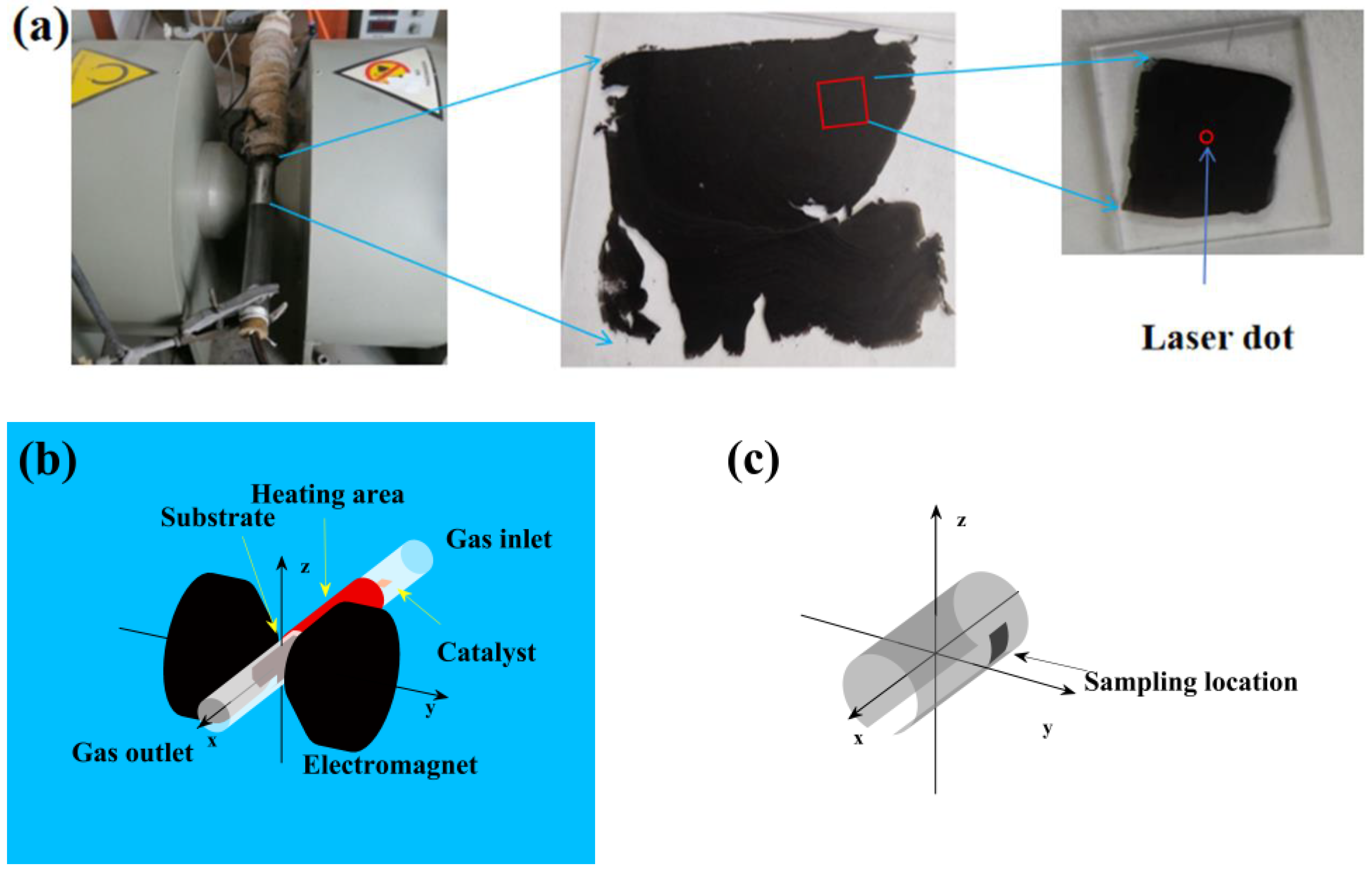
2. Materials and Methods
3. Results
3.1. Characterization
3.2. Carrier Flow
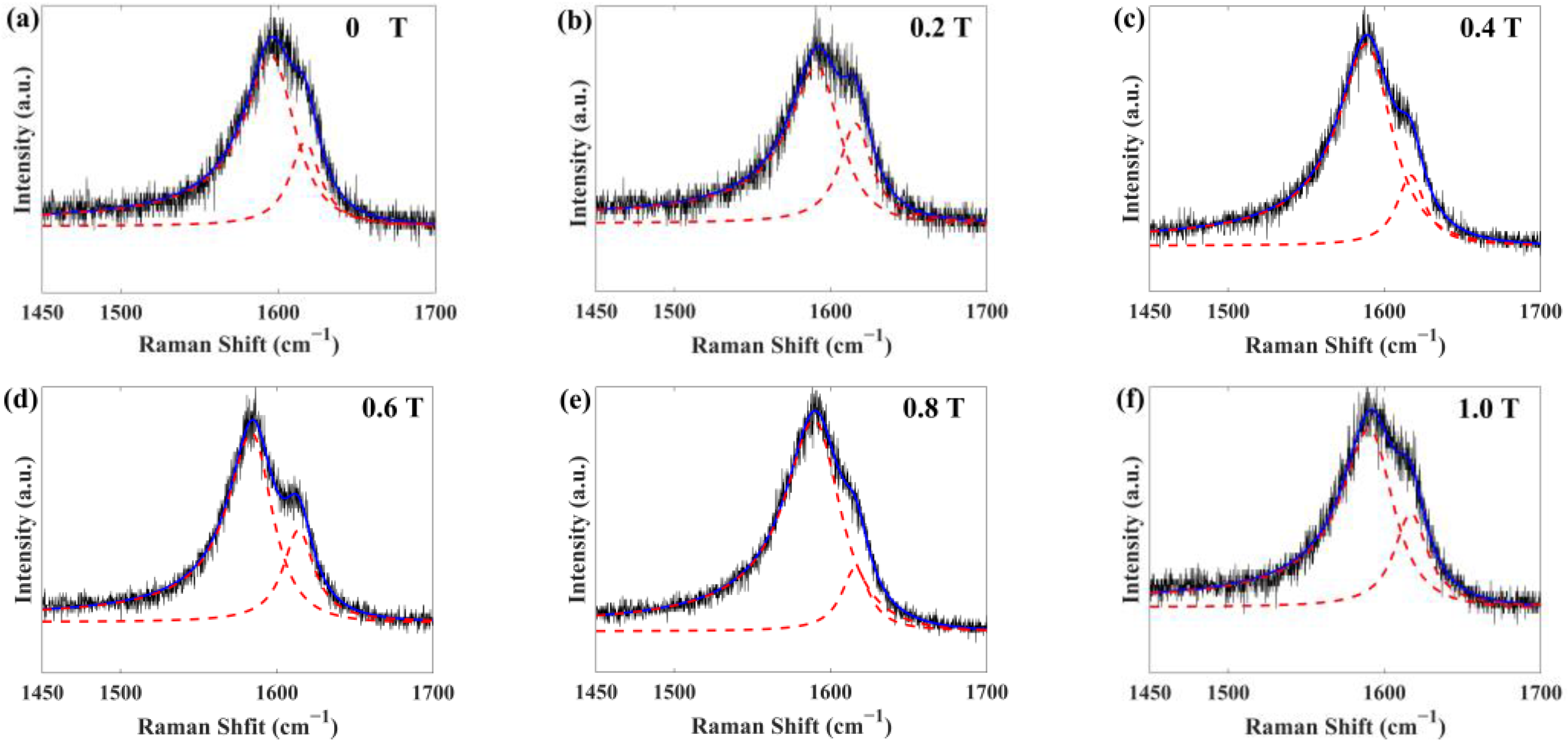
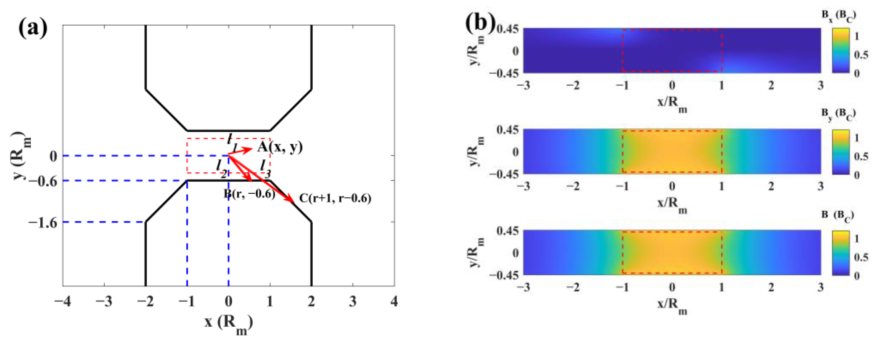
3.3. Magnetic Field
4. Discussion
4.1. Dynamic Analysis of m-SWCNTs Flow
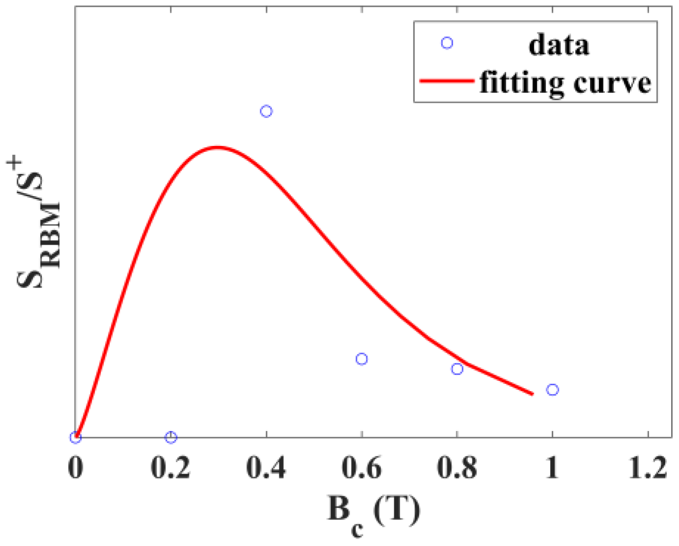
4.2. Calculation of the Axial Magnetic Susceptibility
5. Conclusions
Author Contributions
Funding
Institutional Review Board Statement
Informed Consent Statement
Data Availability Statement
Acknowledgments
Conflicts of Interest
Appendix A

Appendix B


References
- Iijima, S. Helical microtubules of graphitic carbon. Nature 1991, 354, 56–58. [Google Scholar] [CrossRef]
- Saito, R.; Fujita, M.; Dresselhaus, G.; Dresselhaus, M.S. Electronic structure of chiral graphene tubules. Appl. Phys. Lett. 1992, 60, 2204–2206. [Google Scholar] [CrossRef]
- Jianping, L. Novel Magnetic Properties of carbon nanotube. Phys. Rev. Lett. 1995, 74, 1123–1126. [Google Scholar] [CrossRef] [PubMed]
- Ajiki, H.; Ando, T. Magnetic properties of carbon nanotubes. J. Phys. Soc. Jpn. 1993, 62, 2470–2480. [Google Scholar] [CrossRef]
- Ajiki, H.; Ando, T. Magnetic properties of ensembles of carbon nanotubes. J. Phys. Soc. Jpn. 1995, 64, 4382–4391. [Google Scholar] [CrossRef]
- Marques, M.A.L.; d’Avezac, M.; Mauri, F. Magnetic response and NMR spectra of carbon nanotubes from ab initio calculations. Phys. Rev. B 2006, 73, 125433. [Google Scholar] [CrossRef]
- Ma, Y.C.; Lehtinen, P.O.; Foster, A.S.; Nieminen, R.M. Magnetic properties of vacancies in graphene and single-walled carbon nanotubes. New J. Phys. 2004, 6, 68. [Google Scholar] [CrossRef]
- Zaric, S.; Ostojic, G.N.; Kono, J.; Shaver, J.; Moore, V.C.; Strano, M.S.; Hauge, R.H.; Smalley, R.E.; Wei, X. Optical signatures of the Aharonov-Bohm phase in single-walled carbon nanotubes. Science 2004, 304, 1129–1131. [Google Scholar] [CrossRef] [PubMed]
- Islam, M.F.; Milkie, D.E.; Torrens, O.N.; Yodh, A.G.; Kikkawa, J.M. Magnetic heterogeneity and alignment of single wall carbon nanotubes. Phys. Rev. B 2005, 71, 201401. [Google Scholar] [CrossRef]
- Torrens, O.N.; Milkie, D.E.; Ban, B.Y.; Zheng, M.; Onoa, G.B.; Gierke, T.D.; Kikkawa, J.M. Measurement of chiral-dependent magnetic anisotropy in carbon nanotubes. J. Am. Chem. Soc. 2007, 129, 252–253. [Google Scholar] [CrossRef]
- Searle, T.A.; Imanaka, Y.; Takamasu, T.; Ajiki, H.; Fagan, J.A.; Hobbie, E.K.; Kono, J. Large anisotropy in the magnetic susceptibility of metallic carbon nanotubes. Phys. Rev. Lett. 2010, 105, 017403. [Google Scholar] [CrossRef]
- Kim, Y.H.; Torrens, O.N.; Kikkawa, J.M.; Abou-Hamad, E.; Goze-Bac, C.; Luzzi, D.E. High-purity diamagnetic single-wall carbon nanotube buckypaper. Chem. Mater. 2007, 19, 2982–2986. [Google Scholar] [CrossRef]
- Chuxin, W.; Jiaxin, L.; Guofa, D.; Lunhui, G. Removal of ferromagnetic metals for the large-scale purification of single-walled carbon nanotubes. J. Phys. Chem. C 2009, 113, 3612–3616. [Google Scholar] [CrossRef]
- Zaka, M.; Ito, Y.; Wang, H.L.; Yan, W.J.; Robertson, A.; Wu, Y.M.A.; Rümmeli, M.H.; Staunton, D.; Hashimoto, T.; Morton, J.J.L.; et al. Electron Paramagnetic resonance investigation of purified catalyst-free single-walled carbon nanotube. ACS Nano 2010, 4, 7708–7716. [Google Scholar] [CrossRef] [PubMed]
- Nakai, Y.; Tsukada, R.; Miyata, Y.; Saito, T.; Hata, K.; Maniwa, Y. Observation of the intrinsic magnetic susceptibility of highly purified single-wall carbon nanotubes. Phys. Rev. B 2015, 92, 041402. [Google Scholar] [CrossRef]
- Chengzhi, L.; Da, W.; Junji, J.; Delong, L.; Chunxu, P.; Lei, L. A rational design for the separation of metallic and semiconducting single-walled carbon nanotubes using a magnetic field. Nanoscale 2016, 8, 13017–13024. [Google Scholar] [CrossRef] [PubMed]
- Jorio, A.; Saito, R.; Hafner, J.H.; Lieber, C.M.; Hunter, M.; McClure, Y.; Dresselhaus, G.; Dresselhaus, M.S. Structural (n, m) determination of isolated single-wall carbon nanotubes by resonant raman scattering. Phys. Rev. Lett. 2001, 86, 1118–1121. [Google Scholar] [CrossRef]
- LeMieux, M.C.; Roberts, M.; Barman, S.; Jin, Y.M.; Kim, J.M.; Bao, Z.N. Self-sorted, aligned nanotube networks for thin-film transistors. Science 2008, 321, 101–104. [Google Scholar] [CrossRef] [PubMed]
- Brown, S.D.M.; Jorio, A.; Corio, P.; Dresselhaus, M.S.; Dresselhaus, G.; Saito, R.; Kneipp, K. Origin of the Breit-Wigner-Fano lineshape of the tangential G-band feature of metallic carbon nanotubes. Phys. Rev. B 2001, 63, 155414. [Google Scholar] [CrossRef]
- Pavelyev, A.A.; Reshmin, A.I.; Teplovodskii, S.K.; Fedoseev, S.G. On the lower critical Reynolds number for flow in a circular pipe. Fluid Dyn. 2003, 38, 545–551. [Google Scholar] [CrossRef]
- Wang, B.; Ma, Y.F.; Li, N.; Wu, Y.P.; Li, F.F.; Chen, Y.S. Facile and scalable fabrication of well-aligned and closely packed single-walled carbon nanotube films on various substrates. Adv. Mater. 2010, 22, 3067–3070. [Google Scholar] [CrossRef] [PubMed]
- Gspann, T.S.; Smail, F.R.; Windle, A.H. Spinning of carbon nanotube fibres using the floating catalyst high temperature route: Purity issues and the critical role of sulphur. Faraday Discuss. 2014, 173, 47–65. [Google Scholar] [CrossRef] [PubMed]


| T (K) | ||||||||||
|---|---|---|---|---|---|---|---|---|---|---|
| 1223 | 0 | 0.4384 | 1612 | 25.50 | 0.5444 | 1587 | 32.74 | −0.2081 | 17.56 | 26.7 |
| 0.2 | 0.3455 | 1616 | 22.48 | 0.6073 | 1590 | 37.16 | −0.1316 | 12.20 | 34.83 | |
| 0.4 | 0.4223 | 1610 | 28.28 | 0.4967 | 1586 | 31.50 | −0.2168 | 18.76 | 23.42 | |
| 0.6 | 0.3707 | 1613 | 25.26 | 0.5962 | 1587 | 34.36 | −0.1726 | 14.71 | 31.22 | |
| 0.8 | 0.2037 | 1618 | 19.46 | 0.6953 | 1593 | 38.66 | −0.1132 | 6.228 | 41.68 | |
| 1.0 | 0.7784 | 1595 | 28.10 | 0.2432 | 1573 | 41.14 | −0.1536 | 34.36 | 15.35 | |
| 1273 | 0 | 0.2923 | 1617 | 23.44 | 0.5824 | 1598 | 39.22 | −0.1337 | 10.76 | 35.24 |
| 0.2 | 0.3489 | 1616 | 24.86 | 0.5358 | 1594 | 39.52 | −0.1574 | 13.62 | 32.44 | |
| 0.4 | 0.2461 | 1617 | 21.82 | 0.6965 | 1591 | 41.76 | −0.1216 | 8.44 | 45.01 | |
| 0.6 | 0.3214 | 1614 | 24.16 | 0.6501 | 1586 | 35.04 | −0.1311 | 12.20 | 35.17 | |
| 0.8 | 0.2212 | 1616 | 22.00 | 0.7290 | 1592 | 43.60 | −0.1249 | 7.64 | 49.15 | |
| 1.0 | 0.3275 | 1617 | 26.20 | 0.6099 | 1593 | 40.50 | −0.144 | 13.48 | 38.00 | |
| 1323 | 0 | 0.3128 | 1613 | 26.24 | 0.6753 | 1588 | 37.74 | −0.1371 | 12.89 | 39.28 |
| 0.2 | 0.3303 | 1613 | 28.48 | 0.5894 | 1585 | 33.70 | −0.1321 | 14.77 | 30.66 | |
| 0.4 | 0.3177 | 1614 | 26.44 | 0.6397 | 1589 | 37.64 | −0.1495 | 13.19 | 36.98 | |
| 0.6 | 0.3251 | 1610 | 14.00 | 0.5491 | 1584 | 17.32 | −0.1586 | 14.30 | 29.13 | |
| 0.8 | 0.8965 | 1592 | 16.78 | 0.1399 | 1567 | 13.89 | −0.3866 | 47.26 | 5.192 | |
| 1.0 | 0.8340 | 1595 | 16.30 | 0.2513 | 1565 | 25.53 | −0.1833 | 42.71 | 19.48 |
| T (K) | |||||
|---|---|---|---|---|---|
| 1223 | 0 | 0 | |||
| 0.2 | 0 | ||||
| 0.4 | 0 | ||||
| 0.6 | 0.05434 | 193.8 | 17.6 | 1.50 | |
| 0.8 | 0 | ||||
| 1.0 | 0.03577 | 199.4 | 25.8 | 1.45 | |
| 1273 | 0 | 0 | |||
| 0.2 | 0 | ||||
| 0.4 | 0.1149 | 191.3 | 17.7 | 3.193 | |
| 0.6 | 0.05412 | 194.2 | 13.1 | 1.110 | |
| 0.8 | 0.04094 | 194.1 | 22.1 | 1.421 | |
| 1.0 | 0.05828 | 196.4 | 8.2 | 0.746 | |
| 1323 | 0 | 0 | |||
| 0.2 | 0 | ||||
| 0.4 | 0 | ||||
| 0.6 | 0 | ||||
| 0.8 | 0.04209 | 200.8 | 28.52 | 1.886 | |
| 0.04164 | 218.6 | 12.94 | 0.846 | ||
| 1.0 | 0.1005 | 199.8 | 14.83 | 2.341 | |
| 0.05231 | 217.2 | 14.84 | 1.219 |
| s-SWCNTs | 1 | 8 | ||||
| (6, 4)-SWCNTs | 0.69 | 9 | ||||
| (6, 5)-SWCNTs | 0.76 | |||||
| (8, 3)-SWCNTs | 0.78 | |||||
| (7, 5)-SWCNTs | 0.82 | |||||
| (6, 4)-SWCNTs | 300 | 0.69 | 10 | |||
| (6, 5)-SWCNTs | 300 | 0.76 | ||||
| (8, 3)-SWCNTs | 300 | 0.78 | ||||
| (7, 5)-SWCNTs | 300 | 0.83 | ||||
| (6, 6)-SWCNTs | 300 | 0.83 | ||||
| (5, 5)-SWCNTs | 300 | 0.69 | ||||
| (7, 4)-SWCNTs | 300 | 0.77 | ||||
| Purified SWCNTs | 300 | 1.0 | 15 | |||
| Purified SWCNTs | 300 | 1.4 | ||||
| Purified SWCNTs | 300 | 1.9 | ||||
| Purified SWCNTs | 300 | 2.65 | ||||
| Purified SWCNTs and s-SWCNT-rich | 300 | 1.4 | ||||
| Purified SWCNTs and m-SWCNT-rich | 300 | 1.4 | ||||
| m-SWCNTs with defects | 1273 | 1.3 | This work |
Disclaimer/Publisher’s Note: The statements, opinions and data contained in all publications are solely those of the individual author(s) and contributor(s) and not of MDPI and/or the editor(s). MDPI and/or the editor(s) disclaim responsibility for any injury to people or property resulting from any ideas, methods, instructions or products referred to in the content. |
© 2024 by the authors. Licensee MDPI, Basel, Switzerland. This article is an open access article distributed under the terms and conditions of the Creative Commons Attribution (CC BY) license (https://creativecommons.org/licenses/by/4.0/).
Share and Cite
Shen, T.; Fu, Q.; Pan, C. Measurement of the Axial Magnetic Susceptibility of m-SWCNTs at High Temperatures in a Magnetic Field-Assisted FC-CVD. Materials 2024, 17, 2745. https://doi.org/10.3390/ma17112745
Shen T, Fu Q, Pan C. Measurement of the Axial Magnetic Susceptibility of m-SWCNTs at High Temperatures in a Magnetic Field-Assisted FC-CVD. Materials. 2024; 17(11):2745. https://doi.org/10.3390/ma17112745
Chicago/Turabian StyleShen, Tanze, Qiang Fu, and Chunxu Pan. 2024. "Measurement of the Axial Magnetic Susceptibility of m-SWCNTs at High Temperatures in a Magnetic Field-Assisted FC-CVD" Materials 17, no. 11: 2745. https://doi.org/10.3390/ma17112745