
Pulse Design of Constant Strain Rate Loading in SHPB Based on Pulse Shaping Technique

 ,
,  ,
, 
Abstract
1. Introduction
2. Method for Objective Incident Pulse at CSR
2.1. Objective Incident Pulse Model
2.2. Analysis of Stress Uniformity
2.3. Conditions for Constant Strain Rate (CSR) Experiment
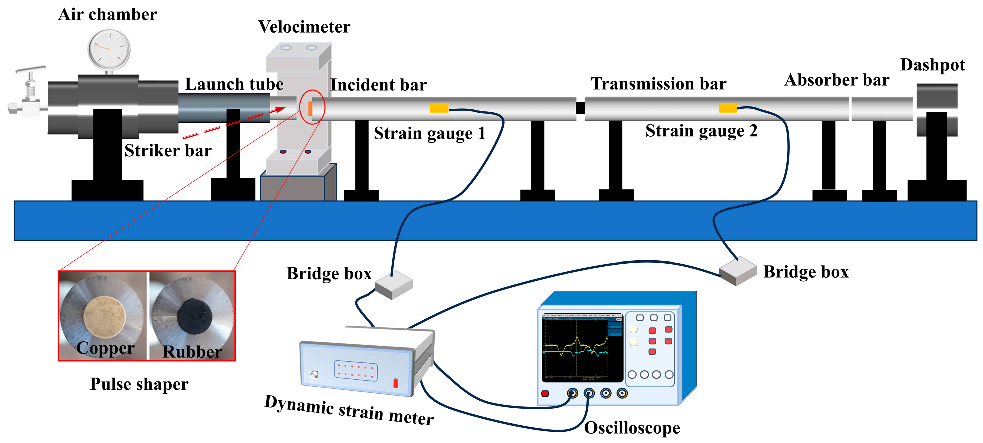
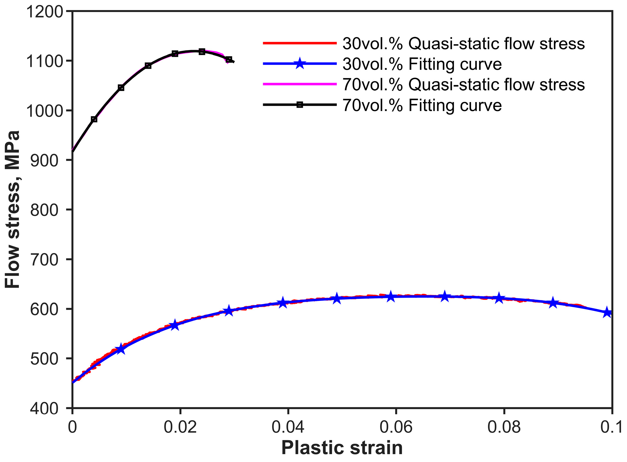
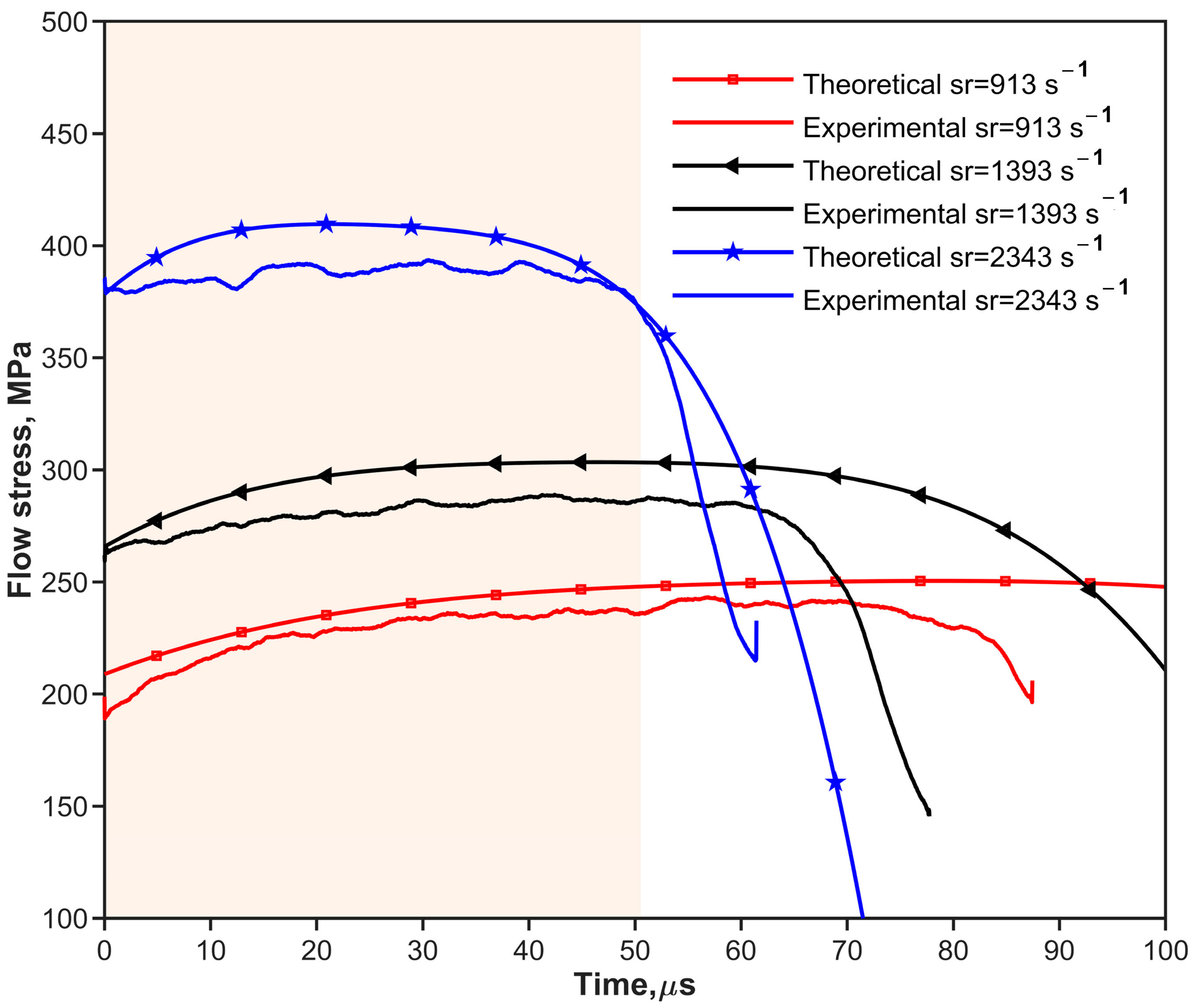
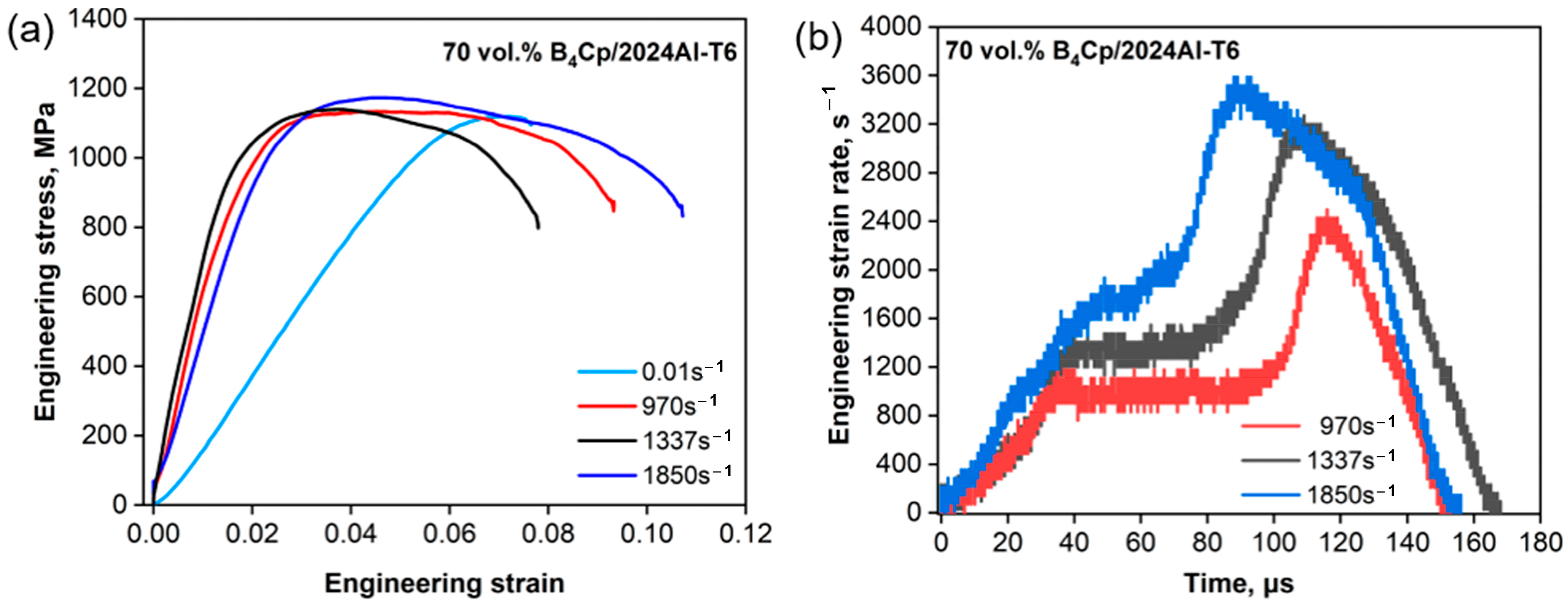
2.4. SHPB CSR Test for B4CP/2024Al Composites
3. Conclusions
- (1)
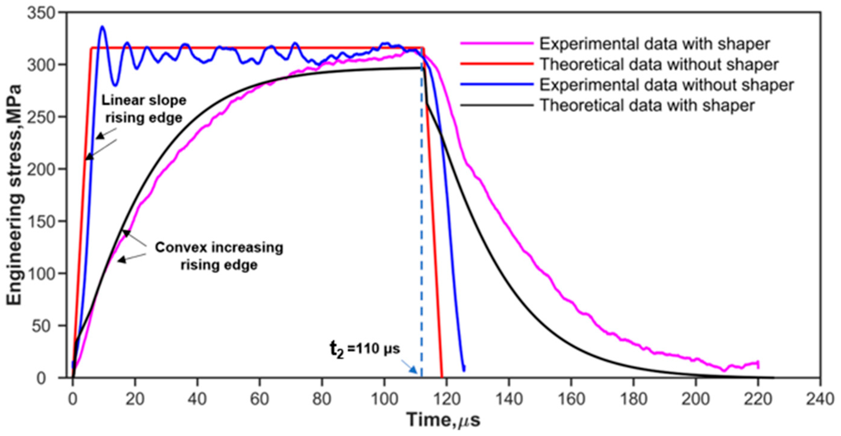
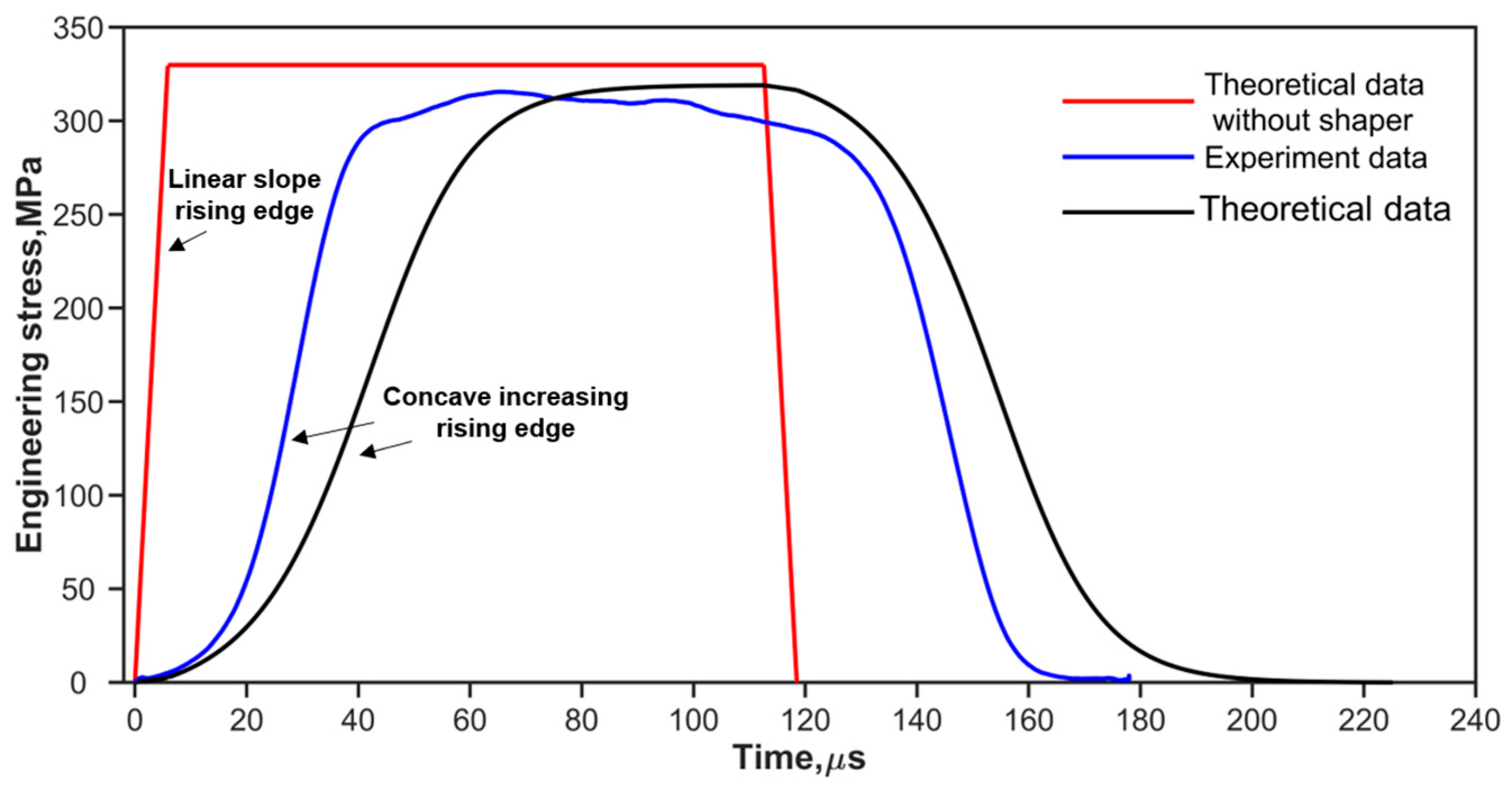
- The objective incident pulse model provides the pulse profile, which is a target for the pulse shaping. One of the obvious differences between the two pulses shaped by the ductile metal shaper (H62 Copper) and the soft shaper (rubber) is the rising edge.
- (2)
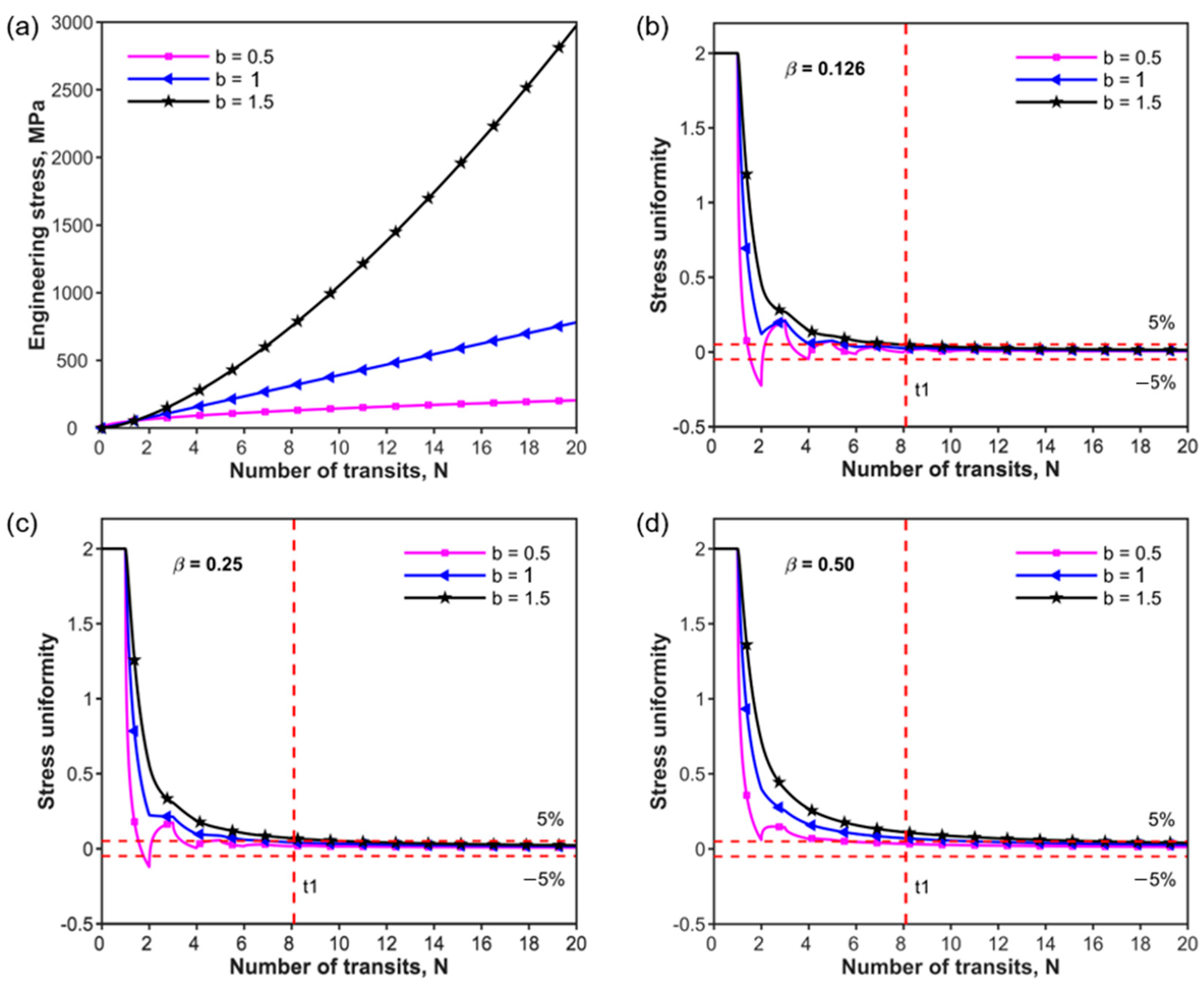
- Stress uniformity during loading is influenced by both the relative mechanical impedance and the rising edge of the incident pulse. Different types of rising edges of the incident pulse do affect the stress uniformity. The time of uniformity increases with the increase in parameter b in the power function.
- (3)
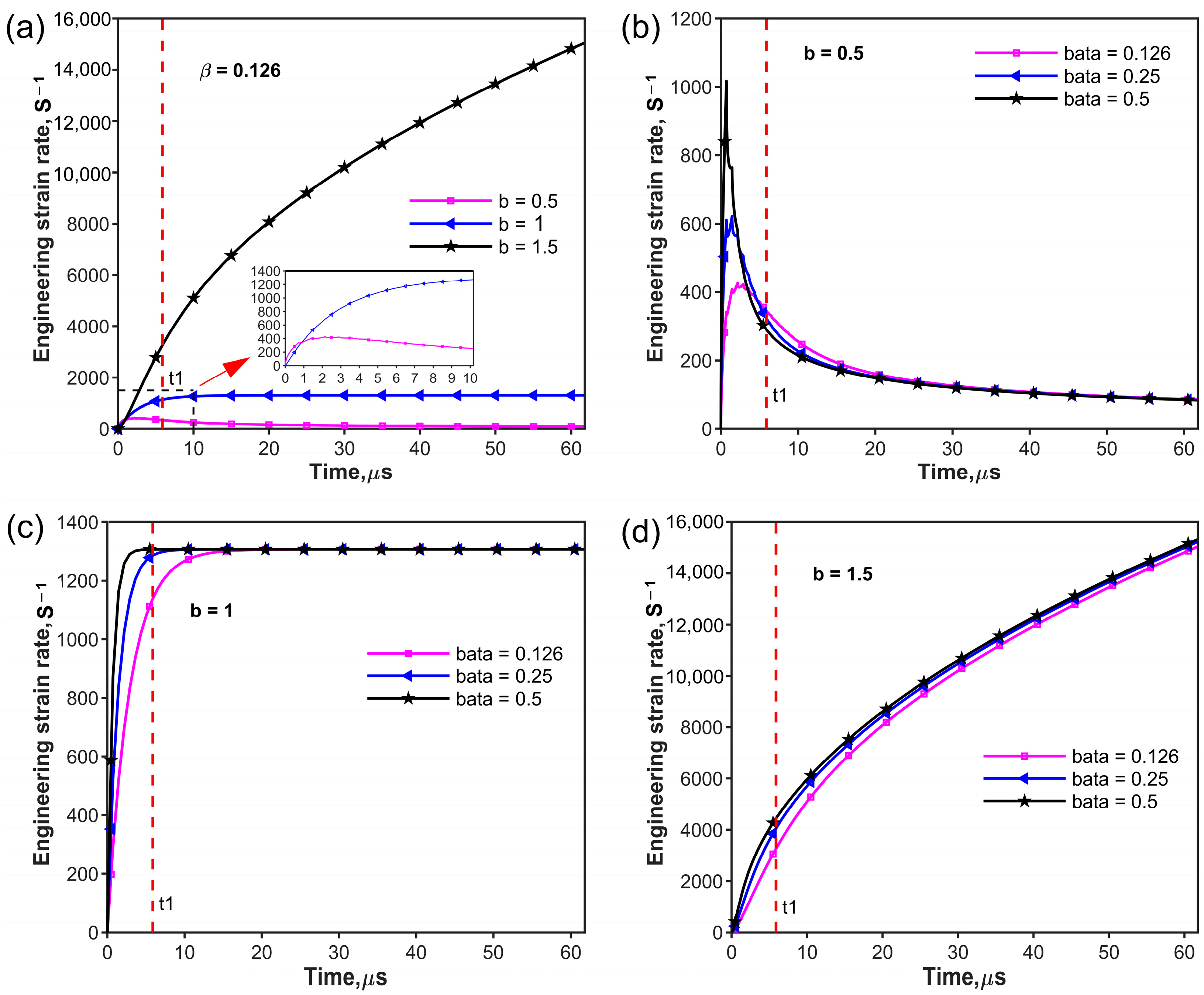
- The rising edge of the incident pulse has a large effect on strain rate history and determines the mode of strain rate–time variations. For the concave rising edge (b = 1.5), the effect of relative mechanical impedance on stress uniformity is negligible, and it is easier to meet the high strain rate loading requirements for the specimen, though the convex increasing (b = 0.5) power law rising edge exhibits favorable characteristics in terms of stress uniformity.
- (4)
- For materials with low strain hardening and strain softening, a negative stress rate pulse facilitates the constant strain rate loading of specimens after experiencing the rising edge of the incident pulse.
Author Contributions
Funding
Institutional Review Board Statement
Informed Consent Statement
Data Availability Statement
Conflicts of Interest
References
- Ramesh, K.T. Effects of high rates of loading on the deformation behavior and failure mechanisms of hexagonal close-packed metals and alloys. Metall. Mater. Trans. A 2002, 33, 927–935. [Google Scholar] [CrossRef]
- Field, J.E.; Walley, S.M.; Proud, W.G.; Goldrein, H.T.; Siviour, C.R. Review of experimental techniques for high rate deformation and shock studies. Int. J. Impact Eng. 2004, 30, 725–775. [Google Scholar] [CrossRef]
- Kolsky, H. An investigation of the mechanical properties of materials at very high rates of loading. Proc. Phys. Soc. Sect. B 1949, 62, 676–700. [Google Scholar] [CrossRef]
- Gama, B.A.; Lopatnikov, S.L.; Gillespie, J.W., Jr. Hopkinson bar experimental technique: A critical review. Appl. Mech. Rev. 2004, 57, 223–250. [Google Scholar] [CrossRef]
- Yang, L.; Shim, V. An analysis of stress uniformity in split Hopkinson bar test specimens. Int. J. Impact Eng. 2005, 31, 129–150. [Google Scholar] [CrossRef]
- Dao, M.; Lu, L.; Shen, Y.; Suresh, S. Strength, strain-rate sensitivity and ductility of copper with nanoscale twins. Acta Mater. 2006, 54, 5421–5432. [Google Scholar] [CrossRef]
- Lee, O.S.; You, S.S.; Chong, J.H.; Kang, H.S. Dynamic deformation under a modified split Hopkinson pressure bar experiment. KSME Int. J. 1998, 12, 1143–1149. [Google Scholar] [CrossRef]
- Vecchio, K.S.; Jiang, F. Improved pulse shaping to achieve constant strain rate and stress equilibrium in split-Hopkinson pressure bar testing. Metall. Mater. Trans. A 2007, 38, 2655–2665. [Google Scholar] [CrossRef]
- Morrow, B.; Lebensohn, R.; Trujillo, C.; Martinez, D.; Addessio, F.; Bronkhorst, C.; Lookman, T.; Cerreta, E. Characterization and modeling of mechanical behavior of single crystal titanium deformed by split-Hopkinson pressure bar. Int. J. Plast. 2016, 82, 225–240. [Google Scholar] [CrossRef]
- Frew, D.J.; Forrestal, M.J.; Chen, W. Pulse shaping techniques for testing brittle materials with a split Hopkinson pressure bar. Exp. Mech. 2002, 42, 93–106. [Google Scholar] [CrossRef]
- Li, X.B.; Lok, T.S.; Zhao, J. Dynamic characteristics of granite subjected to intermediate loading rate. Rock Mech. Rock Eng. 2005, 38, 21–39. [Google Scholar] [CrossRef]
- Liang, X.; Chen, G.; Lei, I.M.; Zhang, P.; Wang, Z.; Chen, X.; Lu, M.; Zhang, J.; Wang, Z.; Sun, T.; et al. Impact-Resistant Hydrogels by Harnessing 2D Hierarchical Structures. Adv. Mater. 2022, 35, 2207587. [Google Scholar] [CrossRef]
- Chao, Z.; Wang, Z.; Jiang, L.; Chen, S.; Pang, B.; Zhang, R.; Du, S.; Chen, G.; Zhang, Q.; Wu, G. Microstructure and mechanical properties of B4C/2024Al functionally gradient composites. Mater. Des. 2022, 215, 110449. [Google Scholar] [CrossRef]
- Woo, S.-C.; Kim, T.-W. High strain-rate failure in carbon/Kevlar hybrid woven composites via a novel SHPB-AE coupled test. Compos. Part B Eng. 2016, 97, 317–328. [Google Scholar] [CrossRef]
- Askarinejad, S.; Johnson, J.E.; Rahbar, N.; Troy, K.L. Effects of loading rate on the of mechanical behavior of the femur in falling condition. J. Mech. Behav. Biomed. Mater. 2019, 96, 269–278. [Google Scholar] [CrossRef]
- Xu, P.; Tang, L.; Zhang, Y.; Ni, P.; Liu, Z.; Jiang, Z.; Liu, Y.; Zhou, L. SHPB experimental method for ultra-soft materials in solution environment. Int. J. Impact Eng. 2022, 159, 104051. [Google Scholar] [CrossRef]
- Jiang, K.; Li, J.; Kan, X.; Zhao, F.; Hou, B.; Wei, Q.; Suo, T. Adiabatic shear localization induced by dynamic recrystallization in an FCC high entropy alloy. Int. J. Plast. 2023, 162, 103550. [Google Scholar] [CrossRef]
- Ellwood, S.; Griffiths, L.J.; Parry, D.J. Materials testing at high constant strain rates. J. Phys. E Sci. Instrum. 1982, 15, 280. [Google Scholar] [CrossRef]
- Parry, D.J.; Walker, A.G.; Dixon, P.R. Hopkinson bar pulse smoothing. Meas. Sci. Technol. 1995, 6, 443. [Google Scholar] [CrossRef]
- Naghdabadi, R.; Ashrafi, M.J.; Arghavani, J. Experimental and numerical investigation of pulse-shaped split Hopkinson pressure bar test. Mater. Sci. Eng. A 2012, 539, 285–293. [Google Scholar] [CrossRef]
- Duffy, J.; Campbell, J.D.; Hawley, R.H. On the use of a torsional split Hopkinson bar to study rate effects in 1100-0 aluminum. J. Appl. Mech. 1971, 38, 83–91. [Google Scholar] [CrossRef]
- Li, X.B.; Lok, T.S.; Zhao, J.; Zhao, P.J. Oscillation elimination in the Hopkinson bar apparatus and resultant complete dynamic stress–strain curves for rocks. Int. J. Rock Mech. Min. Sci. 2000, 37, 1055–1060. [Google Scholar] [CrossRef]
- Li, X.; Zhou, Z.; Lok, T.-S.; Hong, L.; Yin, T. Innovative testing technique of rock subjected to coupled static and dynamic loads. Int. J. Rock Mech. Min. Sci. 2008, 45, 739–748. [Google Scholar] [CrossRef]
- Song, B.; Chen, W. Loading and unloading split Hopkinson pressure bar pulse-shaping techniques for dynamic hysteretic loops. Exp. Mech. 2004, 44, 622–627. [Google Scholar] [CrossRef]
- Li, W.; Xu, J. Impact characterization of basalt fiber reinforced geopolymeric concrete using a 100-mm-diameter split Hopkinson pressure bar. Mater. Sci. Eng. A 2009, 513, 145–153. [Google Scholar] [CrossRef]
- Nemat-Nasser, S.; Isaacs, J.B.; Starrett, J.E. Hopkinson techniques for dynamic recovery experiments. Proc. R. Soc. London Ser. A Math. Phys. Sci. 1991, 435, 371–391. [Google Scholar]
- Frew, D.J.; Forrestal, M.J.; Chen, W. A split Hopkinson pressure bar technique to determine compressive stress-strain data for rock materials. Exp. Mech. 2001, 41, 40–46. [Google Scholar] [CrossRef]
- Frew, D.J.; Forrestal, M.J.; Chen, W. Pulse shaping techniques for testing elastic-plastic materials with a split Hopkinson pressure bar. Exp. Mech. 2005, 45, 186–196. [Google Scholar] [CrossRef]
- Pang, S.; Tao, W.; Liang, Y.; Liu, Y.; Huan, S. A modified method of pulse-shaper technique applied in SHPB. Compos. Part B Eng. 2019, 165, 215–221. [Google Scholar] [CrossRef]
- Ramírez, H.; Rubio-Gonzalez, C. Finite-element simulation of wave propagation and dispersion in Hopkinson bar test. Mater. Des. 2006, 27, 36–44. [Google Scholar] [CrossRef]
- Song, L.; Hu, S. Stress uniformity and constant strain rate in SHPB test. Explos. Shock Waves 2005, 25, 207–216. [Google Scholar]
- Song, L.; Hu, S. Loading designing for constant strain-rate experiment with SHPB. In Proceedings of the Fourth Conference on Experimental Techniques in Explosive Mechanics, Wuyishan, China, 26–27 October 2006; pp. 28–32. [Google Scholar]
- Davies, E.D.H.; Hunter, S.C. The Dynamic Compression Testing of Solids by the Method of the Split Hopkinson Pressure Bar. J. Mech. Phys. Solids 1963, 11, 155–179. [Google Scholar] [CrossRef]
- Lu, F.; Chen, R. Hopkinson Bar Techniques; Science Press: Beijing, China, 2013; pp. 52–58. [Google Scholar]
- Meyers, M.A. Dynamic Behavior of Materials; John Wiley & Sons: Hoboken, NJ, USA, 1994. [Google Scholar]
- Ravichandran, G.; Subhash, G. Critical appraisal of limiting strain rates for compression testing of ceramics in a split Hopkinson pressure bar. J. Am. Ceram. Soc. 1994, 77, 263–267. [Google Scholar] [CrossRef]
- Wang, J.; Ma, L.; Zhao, F.; Lv, B.; Gong, W.; He, M.; Liu, P. Dynamic strain field for granite specimen under SHPB impact tests based on stress wave propagation. Undergr. Space 2022, 7, 767–785. [Google Scholar] [CrossRef]
- Li, Y.; Ramesh, K.; Chin, E. Dynamic characterization of layered and graded structures under impulsive loading. Int. J. Solids Struct. 2001, 38, 6045–6061. [Google Scholar] [CrossRef]
- Johnson, G.R.; Cook, W.H. A constitutive model and data for metals subjected to large strains, high strain rates and high temperatures. In Proceedings of the 7th International Symposium on Ballistics, The Hague, The Netherlands, 19–21 April 1983; pp. 541–547. [Google Scholar]


| Material | Density (g/cm3) | Radius (cm) | Young Module (GPa) | Yield Stress (MPa) | Poisson Ratio | Velocity (m/s) | Thickness (mm) |
|---|---|---|---|---|---|---|---|
| H62 Copper | 8.43 | 0.70 | 131 | 112.0 | 0.31 | 16.0 | 1.00 |
| Rubber | 1.93 | 0.40 | 0.025 | 4.5 | 0.47 | 16.7 | 1.00 |
(Relative Mechanical Impedance) | b (Parameter of Power Law) | ||
|---|---|---|---|
| 0.5 | 1.0 | 1.5 | |
| 0.126 | 3 | 4 | 8 |
| 0.250 | 3 | 7 | 9 |
| 0.500 | 4 | 11 | 14 |
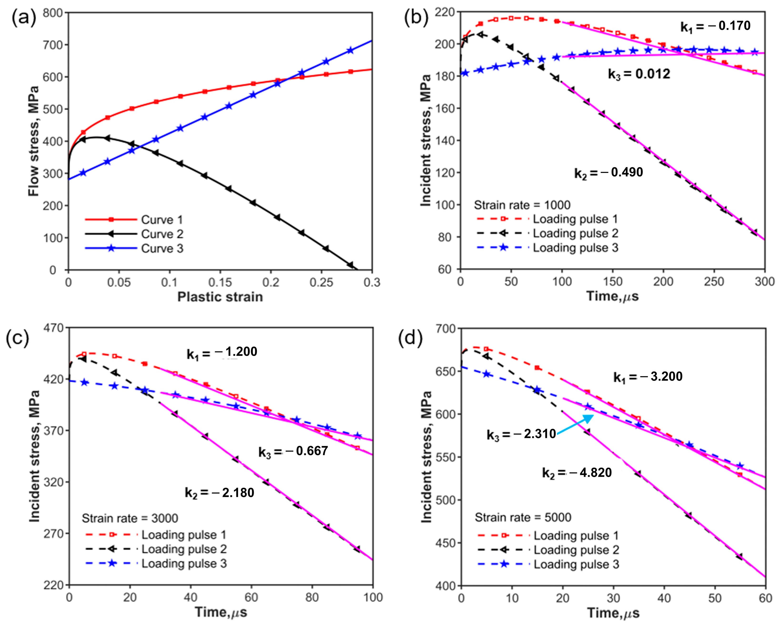
| Curve | a (MPa) | b (MPa) | n1 | c | m |
|---|---|---|---|---|---|
| 1 | 281 | 480 | 0.281 | - | - |
| 2 | 281 | 480 | 0.281 | 3.5 | 1 |
| 3 | 281 | 1440 | 1 | - | - |
| Strain Rate (s−1) | Stress Rate, (MPa/us) | ||
|---|---|---|---|
| k1 | k2 | k3 | |
| 1000 | −0.170 | −0.490 | 0.012 |
| 3000 | −1.200 | −2.180 | −0.667 |
| 5000 | −3.200 | −4.820 | −2.310 |
| B4Cp/2024Al Composites | 30 vol.% | 70 vol.% | ||||
|---|---|---|---|---|---|---|
| Shaper Materials | Copper | Rubber | ||||
| Sz of the Shaper, mm | Ø11 × 1 | Ø4 × 1 | Ø4 × 1.5 | |||
| Sr, s−1 | 913 | 1393 | 2343 | 970 | 1337 | 1850 |
| Theo.V, m/s | 11.10 | 14.10 | 20.10 | 16.36 | 19.36 | 22.36 |
| Exp.V, m/s | 12.30 | 15.75 | 20.55 | 16.96 | 19.06 | 21.15 |
| B4Cp/2024Al Composites | Density (g/cm3) | Young Module (GPa) | Yield Stress (MPa) | Wave Speed (m/s) | Radius (mm) | Thickness (mm) |
|---|---|---|---|---|---|---|
| 30 vol% | 2.70 | 184 | 451 | 10,240 | 6 | 6 |
| 70 vol% | 2.60 | 336 | 917 | 11,966 | 6 | 6 |
Disclaimer/Publisher’s Note: The statements, opinions and data contained in all publications are solely those of the individual author(s) and contributor(s) and not of MDPI and/or the editor(s). MDPI and/or the editor(s) disclaim responsibility for any injury to people or property resulting from any ideas, methods, instructions or products referred to in the content. |
© 2024 by the authors. Licensee MDPI, Basel, Switzerland. This article is an open access article distributed under the terms and conditions of the Creative Commons Attribution (CC BY) license (https://creativecommons.org/licenses/by/4.0/).
Share and Cite
Chen, S.; Chi, R.; Cao, W.; Pang, B.; Chao, Z.; Jiang, L.; Luo, T.; Zhang, R. Pulse Design of Constant Strain Rate Loading in SHPB Based on Pulse Shaping Technique. Materials 2024, 17, 2931. https://doi.org/10.3390/ma17122931
Chen S, Chi R, Cao W, Pang B, Chao Z, Jiang L, Luo T, Zhang R. Pulse Design of Constant Strain Rate Loading in SHPB Based on Pulse Shaping Technique. Materials. 2024; 17(12):2931. https://doi.org/10.3390/ma17122931
Chicago/Turabian StyleChen, Shengpeng, Runqiang Chi, Wuxiong Cao, Baojun Pang, Zhenlong Chao, Longtao Jiang, Tian Luo, and Runwei Zhang. 2024. "Pulse Design of Constant Strain Rate Loading in SHPB Based on Pulse Shaping Technique" Materials 17, no. 12: 2931. https://doi.org/10.3390/ma17122931
APA StyleChen, S., Chi, R., Cao, W., Pang, B., Chao, Z., Jiang, L., Luo, T., & Zhang, R. (2024). Pulse Design of Constant Strain Rate Loading in SHPB Based on Pulse Shaping Technique. Materials, 17(12), 2931. https://doi.org/10.3390/ma17122931