
The Impact of Dynamic Effects on the Results of Non-Destructive Falling Weight Deflectometer Testing
Abstract
1. Introduction
2. Materials and Methods
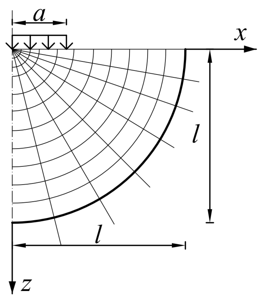
2.1. Pavement Subjected to Rapidly Changing Load
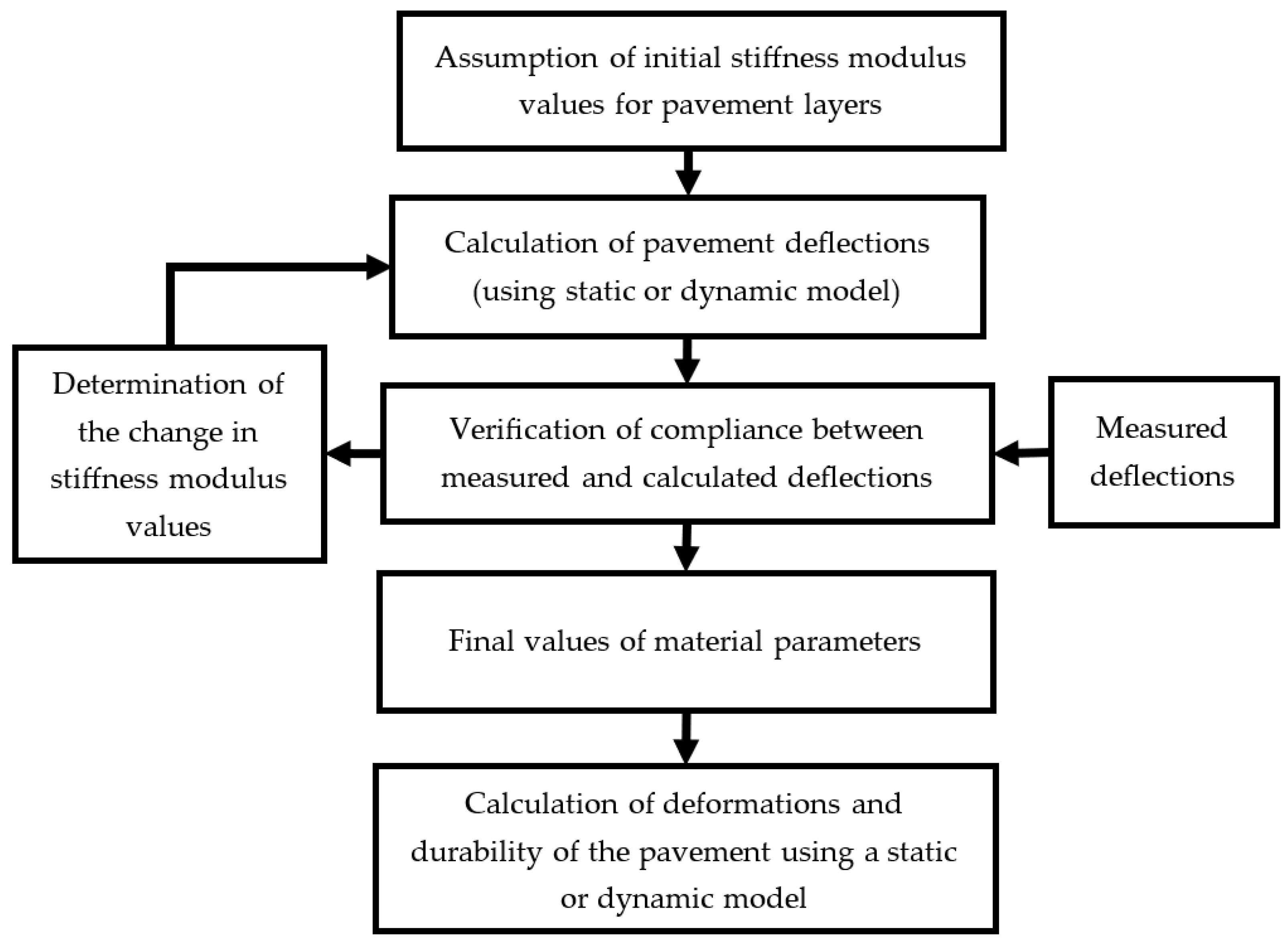
2.2. Backcalculation Scheme
3. Results
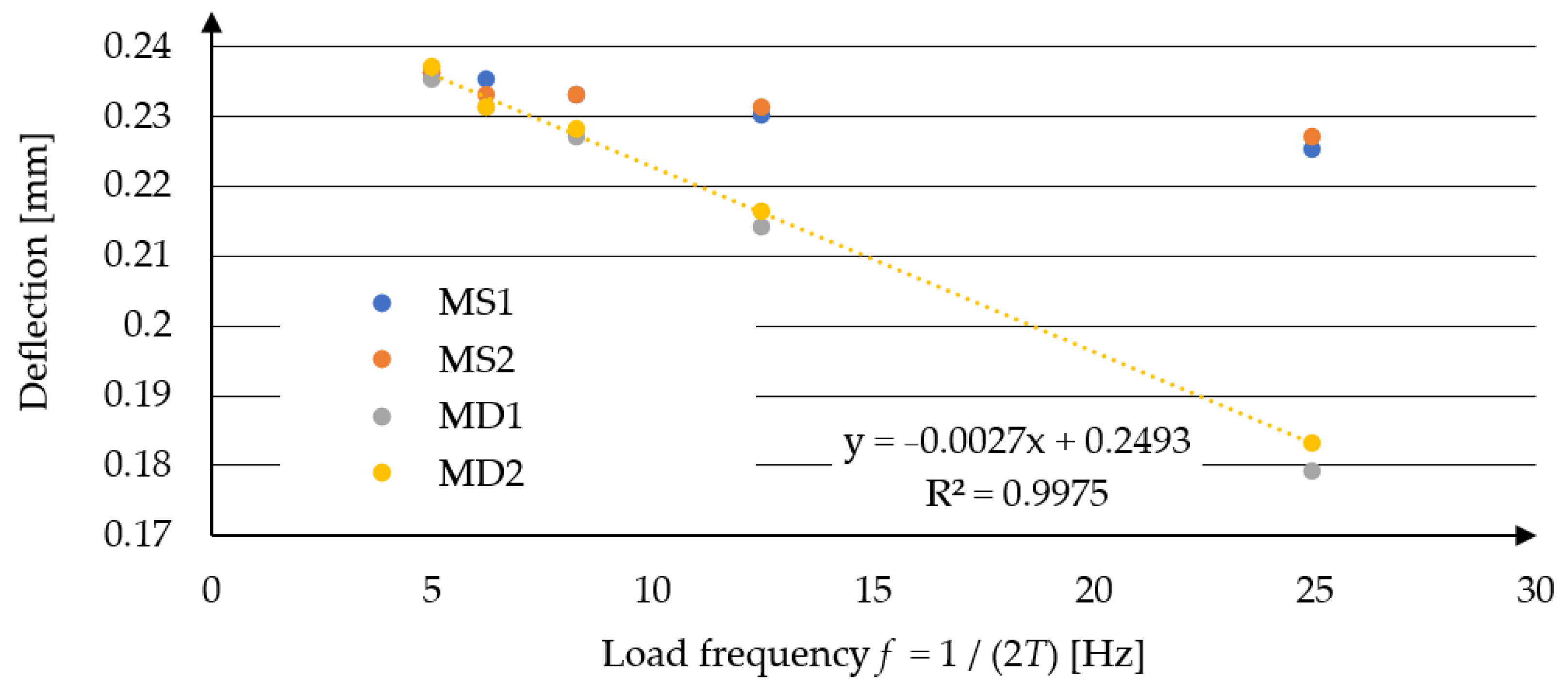
3.1. Computed Deflection Results for Rapidly Changing Loads
3.2. The Impact of Dynamic Effects on Backcalculation
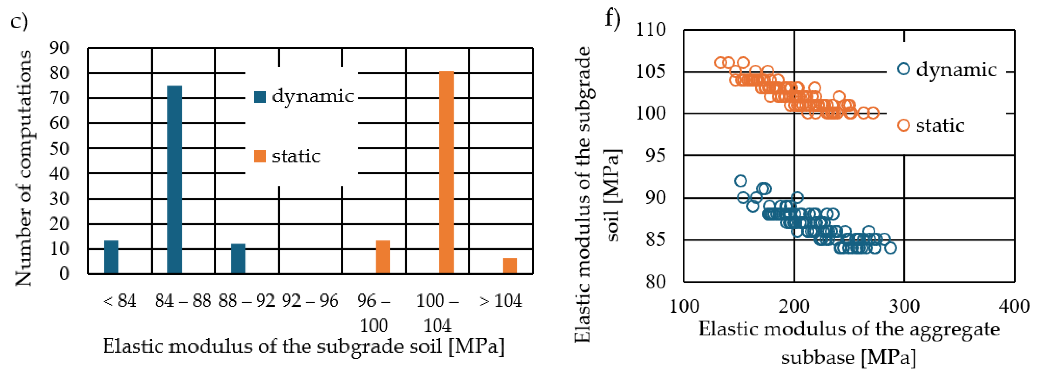
3.2.1. Calculation Results—Elastic Modulus Values
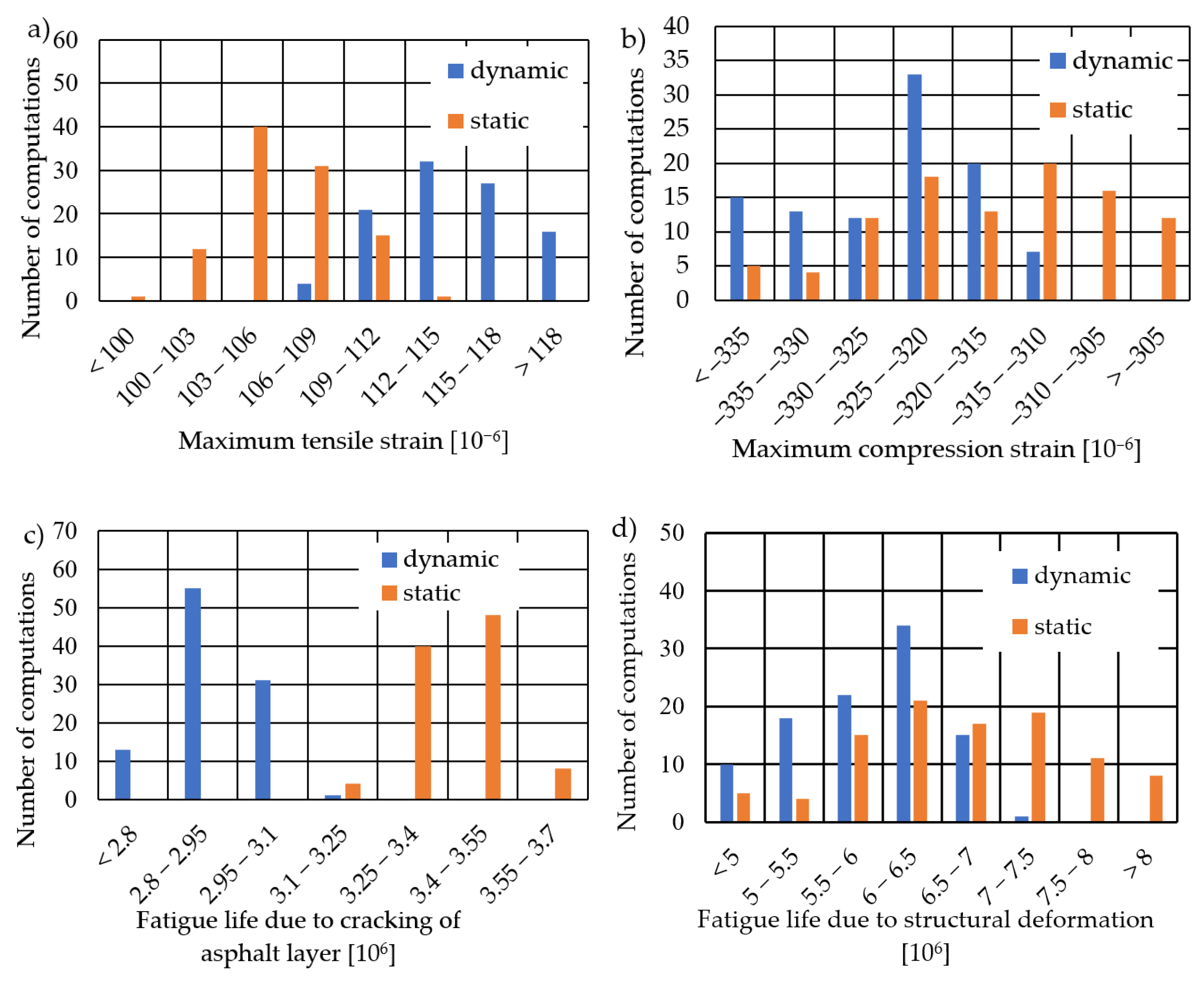
3.2.2. Critical Deformation Values and Fatigue Life Predictions
4. Discussion
- When dealing with rapidly varying loads, it is crucial to use a dynamic model that incorporates inertia forces due to the finite propagation time of deformation waves in the pavement. This is particularly significant for loading durations of 0.04 s or less.
- The use of a linearly elastic model for asphalt layers, employing the dynamic modulus as the elastic modulus, can lead to differences in calculation results compared to a viscoelastic model (though not as significant as when dynamic effects are omitted altogether). This discrepancy arises from the challenge of accurately determining the material’s load frequency when assessing the dynamic modulus.
- Backcalculation for FWD tests should be performed using a dynamic model. The use of a static model introduces significant discrepancies in the results.
- In diagnostic tests, results obtained within the loading duration range of 0.02 to 0.06 s should be normalized due to the duration of force application. Deflection calculation results for the same pavement and maximum load can vary significantly depending on the loading time; for example, the maximum deflection difference for the MD2 model is 25% between calculations for loading durations of 0.02 s and 0.06 s. This is important when using the so-called representative deflection obtained during FWD tests as a measure of bearing capacity in road condition diagnostics.
- When applying backcalculation, the sensitivity of results to the measured deflection values is crucial. Similar input data can lead to different combinations of material parameters, subsequently affecting critical strains and pavement fatigue life.
- Analysing the sensitivity of fatigue life results due to bottom-up asphalt layer cracking and permanent deformation shows significantly greater sensitivity in the latter case (with a coefficient of variation of 13.7% for static and 10.5% for dynamic calculations). This is due to the amplification of strain variability through the fatigue life equation, which involves approximately the fourth power of the strain. The variability in the fatigue life of asphalt layers is somewhat mitigated by considering the stiffness of asphalt layers in the fatigue life formula.
- The elastic moduli of the asphalt layers and the base course exhibit particularly high sensitivity in the results. In the study, where errors were relatively small and generated randomly, these values are strongly negatively correlated (−0.97). This means that when one value is relatively high, the other is lower. A closer analysis of the correlation between individual deflections and moduli reveals that higher stiffness of the upper layers is obtained for flatter deflection basins, while higher stiffness of the base course occurs in steeper deflection basins. This suggests that the calculations are particularly sensitive to changes in the shape of the deflection basin. The variability in elastic moduli Ea and Eb was primarily influenced by deflections at the first four points (located at distances of 0 cm, 20 cm, 30 cm, and 60 cm from the load axis). This effect is similar in backcalculations performed using dynamic and static calculations.
- The subgrade soil’s elastic modulus depends primarily on deflections farther from the load axis. The importance coefficient from the Random Forest model is 30% for dynamic calculations and 43% for static calculations. It is important to note that the variability of the determined soil modulus is significantly lower than that of other layers, making it less sensitive to random measurement errors. However, there is a consistent difference between the soil’s elastic modulus obtained in backcalculation using static and dynamic models due to the different shapes of the deflection basin in the various computational models.
- Comparing the sensitivity between static and dynamic results does not reveal significant qualitative differences. In static model calculations, the shape of the deflection basin is slightly different from that in dynamic calculations, which slightly alters the numerical relationships between deflections and the outcome values in the backcalculation process.
- From the perspective of backcalculation sensitivity within a single measurement point, multiple measurements should be conducted to determine the actual variability of deflection results, which could be used in further data processing. The number of measurements should depend on the observed variability and the required accuracy. The average value obtained from multiple measurements would be a more reliable figure for further calculations.
- When performing backcalculations, the observed variability in deflections from multiple measurements should be considered, and this variability should be modelled accordingly, similar to the approach used in this study.
- When performing backcalculations with determined errors, the result should include confidence intervals or envelopes for the elastic moduli. The outcome of backcalculation should provide ranges of elastic modulus values along with the dependencies between the elastic moduli of individual layers.
- The calculations were performed for a pavement structure with given layer thicknesses. It would be advisable to generalize the conclusions to a broader range of possible cases.
- The numerical models used in the calculations require experimental validation. Moreover, the adopted method for obtaining stiffness moduli in backcalculations should always be verified by independent measurement methods.
- The study presents considerations on the impact of using static and dynamic models in backcalculation on the resulting elasticity moduli and, consequently, on how changes in these moduli affect the estimated remaining fatigue life of the pavement structure. A separate issue is the consideration of inertia forces in both the pavement structure and the heavy vehicle moving on the pavement during calculations to determine pavement deformations, which are then used in fatigue life calculations. Including this aspect would provide a more complete picture of the difference in results when using static versus dynamic models.
- The study of pavement behaviour with a high-stiffness material layer (“bedrock”) located at a relatively shallow depth beneath the road surface. In such pavements, the influence of dynamic effects may be qualitatively different due to the reflection of waves within the flexible medium from the stiff layer. In this scenario, deflections calculated using a dynamic model might be larger than those predicted by a static model.
- The use of time-dependent deflection values in backcalculation to determine the viscoelastic parameters of asphalt layer models. In theory, analysing the time history of deflection curves should allow for the determination of viscoelastic parameters. However, the challenge lies in the potentially heightened sensitivity of such calculations to variations in the measured deflections.
- Determination of other pavement structural parameters, such as layer thickness and Poisson’s ratios, where the sensitivity of the results to relatively small changes in input data remains a significant issue.
- The application of artificial neural networks for objective function minimization in backcalculation procedures.
Author Contributions
Funding
Institutional Review Board Statement
Informed Consent Statement
Data Availability Statement
Conflicts of Interest
Abbreviations
| p(t) | the value of the pressure loading the pavement at time t [kPa] |
| p0 | maximum load pressure [kPa] |
| T | loading time [s] |
| a | radius of the circular load area [m] |
| f | load frequency [Hz] |
| ω | loading angular frequency [rad/s] |
| E* | complex modulus |
| i | imaginary unit |
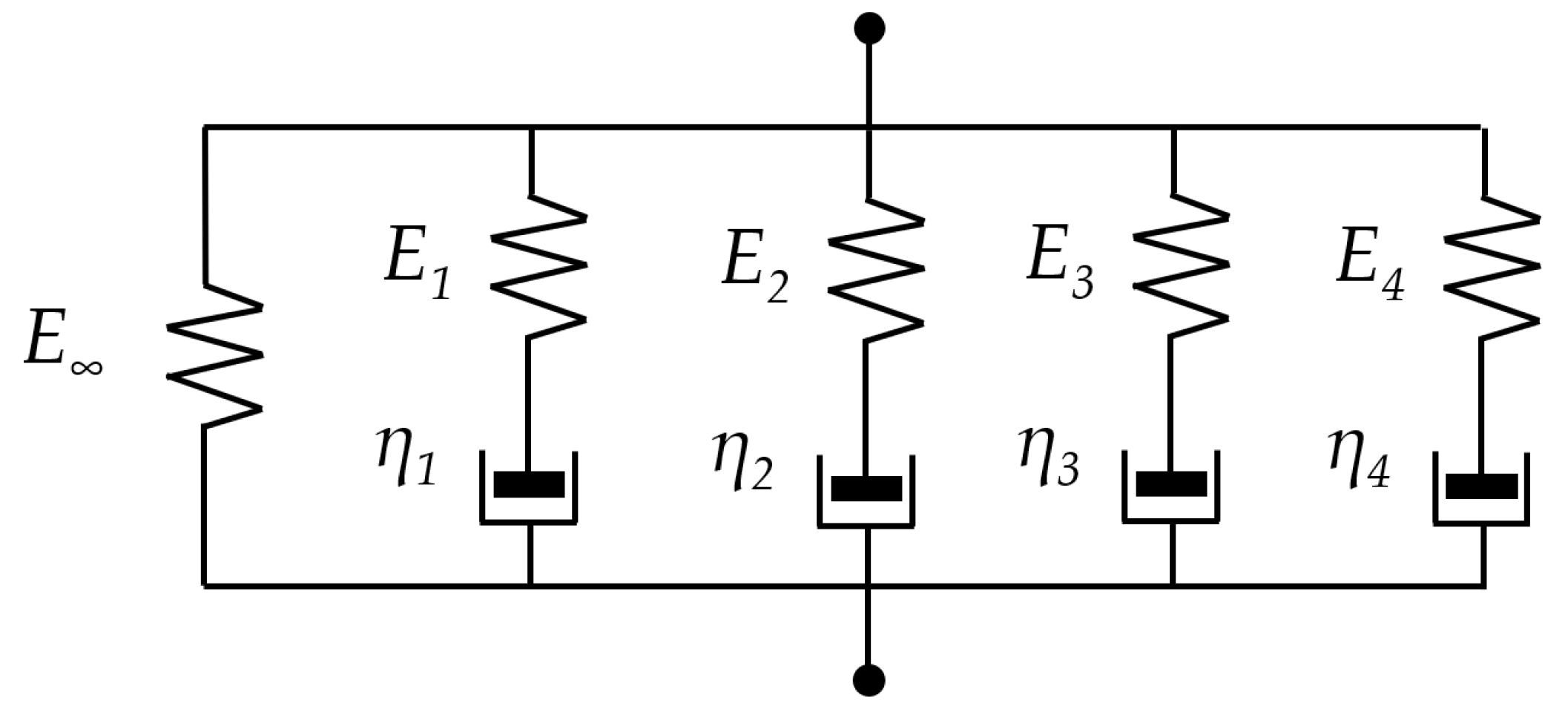
| E0, E∞, E1, E2, E3, E4 | parameters (stiffnesses) in the generalized Maxwell model [MPa] |
| η1, η2, η3, η4 | parameters (viscous damper) in generalized Maxwell model [MPa·s] |
| g1, g2, g3, g4 | dimensionless parameters in the generalized Maxwell model [-] |
| τ1, τ2, τ3, τ4 | retardation times, parameters in generalized Maxwell model [s] |
| Ea | elastic modulus of asphalt layer [MPa] |
| Eb | elastic modulus of subbase [MPa] |
| Ec | elastic modulus of subgrade [MPa] |
| u1, u2, u3, u4, u5, u6, u7 | Deflections measured at the first, second, …, and seventh points during the FWD testing [mm] |
| RSME | root square mean error |
| ρ | density of material [kg/m3] |
| ν | Poisson ratio [-] |
| εh | maximum tensile strain at the bottom of asphalt layer [10−6] |
| εv | maximum compression strain at the surface of the subgrade [10−6] |
| Va | asphalt volume content of asphalt layer [%] |
| Vv | void volume content of asphalt layer [%] |
| Nf | the fatigue life of the pavement due to fatigue bottom-up cracking of the asphalt layer [mln of 100 kN axes] |
| Nd | fatigue life due to structural fatigue deformations [mln of 100 kN axes] |
References
- Radzikowski, M.; Foryś, G. Diagnostyka stanu nawierzchni i wybranych elementów korpusu drogowego. Drogownictwo 2020, 3, 73–89. [Google Scholar]
- Judycki, J.; Jaskuła, P.; Pszczoła, M.; Ryś, D.; Jaczewski, M.; Alenowicz, J.; Dołżycki, B.; Stienss, M. Analizy i projektowanie konstrukcji nawierzchni podatnych i półsztywnych. Wydaw. Komun. I Łączności 2014, 18, 250–302. [Google Scholar]
- Kutay, M.E.; Chatti, K.; Lei, L. Backcalculation of dynamic modulus mastercurve from falling weight deflectometer surface deflections. Transp. Res. Rec. 2011, 2227, 87–96. [Google Scholar] [CrossRef]
- Hadidi, R.; Gucunski, N. Comparative study of static and dynamic falling weight deflectometer back-calculations using probabilistic approach. J. Transp. Eng. 2010, 136, 196–204. [Google Scholar] [CrossRef]
- Huang, Y.H. Pavement Analysis and Design, 2nd ed.; Prentice-Hall: Upper Saddle River, NJ, USA, 2004. [Google Scholar]
- Smith, K.D.; Bruinsma, J.E.; Wade, M.J.; Chatti, K.; Vandenbossche, J.M.; Yu, H.T. Using Falling Weight Deflectometer Data with Mechanistic-Empirical Design and Analysis, Volume I: Final Report; Report No. FHWA-HRT-16-009; Federal Highway Administration: Washington, WA, USA, 2017.
- Bruinsma, J.E.; Vandenbossche, J.; Chatti, K.; Smith, K.D. Using Falling Weight Deflectometer Data with Mechanistic-Empirical Design and Analysis, Volume II: Case Study Reports; Federal Highway Administration: Washington, WA, USA, 2017.
- Pierce, L.M.; Bruinsma, J.E.; Smith, K.D.; Wade, M.J.; Chatti, K.; Vandenbossche, J. Using Falling Weight Deflectometer Data With Mechanistic-Empirical Design and Analysis, Volume III: Guidelines for Deflection Testing, Analysis, and Interpretation; Federal Highway Administration: Washington, WA, USA, 2017.
- Chatti, K.; Kutay, M.E.; Lajnef, N.; Zaabar, I.; Varma, S.; Lee, H.S. Enhanced Analysis of Falling Weight Deflectometer Data for Use with Mechanistic-Empirical Flexible Pavement Design and Analysis and Recommendations for Improvements to Falling Weight Deflectometers; Turner-Fairbank Highway Research Center: McLean, VA, USA, 2017.
- Sebaaly, B.E.; Mamlouk, M.S.; Davies, T.G. Dynamic analysis of falling weight deflectometer data. Transp. Res. Rec. 1986, 1070, 63–68. [Google Scholar]
- Roesset, J.M.; Shao, K.Y. Dynamic interpretation of dynaflect and falling weight deflectometer tests. Transp. Res. Rec. 1985, 1022, 7–16. [Google Scholar]
- Garg, N.; Marsey, W.H. Comparison between falling weight deflectometer and static deflection measurements on flexible pavements at the National Airport Pavement Test Facility (NAPTF). In Proceedings of the CD-ROM 2002 FAA Airport Technology Transfer Conference, Atlantic City, NJ, USA, 5–8 May 2002. [Google Scholar]
- Seo, J.W.; Kim, S.I.; Choi, J.S.; Park, D.W. Evaluation of layer properties of flexible pavement using a pseudo-static analysis procedure of Falling Weight Deflectometer. Constr. Build. Mater. 2009, 23, 3206–3213. [Google Scholar] [CrossRef]
- El Ayadi, A.; Picoux, B.; Lefeuve-Mesgouez, G.; Mesgouez, A.; Petit, C. An improved dynamic model for the study of a flexible pavement. Adv. Eng. Softw. 2012, 44, 44–53. [Google Scholar] [CrossRef]
- Li, M.; Wang, H.; Xu, G.; Xie, P. Finite element modeling and parametric analysis of viscoelastic and nonlinear pavement responses under dynamic FWD loading. Constr. Build. Mater. 2017, 141, 23–35. [Google Scholar] [CrossRef]
- Nazarian, S.; Boddapati, K.M. Pavement-falling weight deflectometer interaction using dynamic finite-element analysis. Transp. Res. Rec. 1995, 1482, 33. [Google Scholar]
- Lee, H.S. Viscowave-A new solution for viscoelastic wave propagation of layered structures subjected to an impact load. Int. J. Pavement Eng. 2014, 15, 542–557. [Google Scholar] [CrossRef]
- Pożarycki, A.; Górnaś, P.; Wanatowski, D. The influence of frequency normalisation of FWD pavement measurements on backcalculated values of stiffness moduli. Road Mater. Pavement Des. 2019, 20, 1–19. [Google Scholar] [CrossRef]
- Tutka, P.; Nagórski, R.; Złotowska, M. Backcalculation of flexible pavement moduli including interlayer bonding conditions–numerical analysis. Arch. Civ. Eng. 2022, 68, 5–22. [Google Scholar]
- Haponiuk, B.; Zbiciak, A. Mechanistic-empirical asphalt pavement design considering the effect of seasonal temperature variations. Arch. Civ. Eng. 2016, 62, 35–50. [Google Scholar]
- Siddharthan, R.; Sebaaly, P.E.; Javaregowda, M. Influence of statistical variation in falling weight deflectometers on pavement analysis. Transp. Res. Rec. 1992, 1377, 57. [Google Scholar]
- Tutka, P.; Nagórski, R.; Złotowska, M.; Rudnicki, M. Sensitivity analysis of determining the material parameters of an asphalt pavement to measurement errors in backcalculations. Materials 2021, 14, 873. [Google Scholar] [CrossRef] [PubMed]
- Breiman, L. Random forests. Mach. Learn. 2001, 45, 5–32. [Google Scholar] [CrossRef]
- Hibbitt, H.; Karlsson, B.; Sorensen, P. Abaqus Analysis User’s Manual, version 6.14; Dassault Systèmes Simulia Corp.: Johnston, RI, USA, 2011. [Google Scholar]
- Nagórski, R.; Tutka, P.; Złotowska, M. Dobór obszaru i warunków brzegowych modelu nawierzchni drogowej podatnej w analizie metodą elementów skończonych. Roads Bridges/Drog. I Mosty, 2017; 16, 271. [Google Scholar]
- Nagórski, R.T.; Błażejowski, K.; Nagórska, M. Studium właściwości mechanicznych konstrukcji nawierzchni drogowej podatnej z uwzględnieniem trwałości: Zagadnienia wybrane. Ser. Stud. I Rozpr. Nr 87 Kom. Inżynierii Lądowej I Wodnej Pol. Akad. Nauk. 2014, 87, 1–141. [Google Scholar]
- PN-EN 12697-26:2018-08; Mieszanki Mineralno-Asfaltowe-Metody Badań-Część 26: Sztywność. Polski Komitet Normalizacyjny: Warsaw, Poland, 2018.
- AASHTO. Mechanistic-Empirical Pavement Design Guide: A Manual of Practice; AASHTO: Washington, DC, USA, 2008. [Google Scholar]
- Claessen, A.; Edwards, J.M.; Sommer, P.; Uge, P. Asphalt pavement design—The shell method. In Volume I of Proceedings of the 4th International Conference on Structural Design of Asphalt Pavements, Ann Arbor, MI, USA, 22–26 August 1977; University of Michigan: Ann Arbor, MI, USA, 1977. [Google Scholar]


| No | Parameter Description | Symbol | Value | Units |
|---|---|---|---|---|
| 1. | The value of pressure at time t | p(t) | ranging from 0 to 707 | kPa |
| 2. | Maximum load pressure | p0 | 707 | kPa |
| 3. | Time loadings | T | five cases were considered: 0.1, 0.08, 0.06, 0.04, 0.02 | s |
| 4. | Time variable | t | variables ranging from 0 to T | s |
| 5. | The radius of the circular load surface | a | 0.15 | m |
| 6. | Load frequencies | f | five cases were considered: 5, 6.25, 8.33, 12.5, 25 | Hz |
| No | Model Description | Model Designation | Inclusion of Inertia Forces | Modelling Approach for Asphalt Layer Properties |
|---|---|---|---|---|
| 1. | Static Model | MS1 | No | Linearly elastic model. Dynamic modulus at a given frequency of loading as the elastic modulus of the layer. |
| 2. | Quasi-Static Model | MS2 | No | Viscoelastic model. Properties are defined using a Prony series. |
| 3. | Dynamic Model | MD1 | Yes | Linearly elastic model. Dynamic modulus at a given frequency of loading as the elastic modulus of the layer. |
| 4. | Dynamic Model | MD2 | Yes | Viscoelastic model. Properties are defined using a Prony series. |
| No. | Frequency [Hz] | E [MPa] for −2 °C | E [Mpa] for 10 °C | E [Mpa] for 23 °C |
|---|---|---|---|---|
| 1. | 0.1 | 13,748 | 7721 | 3357 |
| 2. | 0.2 | 14,789 | 8546 | 3836 |
| 3. | 0.5 | 16,044 | 9695 | 4576 |
| 4. | 1.0 | 17,022 | 10,596 | 5206 |
| 5. | 2.0 | 18,002 | 11,534 | 5900 |
| 6. | 5.0 | 19,293 | 12,806 | 6904 |
| 7. | 8.0 | 19,988 | 13,483 | 7465 |
| 8. | 10.0 | 20,326 | 13,818 | 7728 |
| 9. | 20.0 | 21,229 | 14,795 | 8607 |
| 10. | 30.0 | 21,807 | 15,358 | 9124 |
| No. | Parameter Name | Parameter Value |
|---|---|---|
| 1. | E0 [Mpa] | 15,839.4 |
| 2. | g1 [1] | 0.198833 |
| 3. | g2 [1] | 0.177083 |
| 4. | g3 [1] | 0.167500 |
| 5. | g4 [1] | 0.455187 |
| 6. | τ1 [s] | 0.011212 |
| 7. | τ2 [s] | 0.082304 |
| 8. | τ3 [s] | 0.664383 |
| 9. | τ4 [s] | 97.0579 |
| 10. | RSME of Ed [Mpa] | 41.09 |
| No | Layer | h [cm] | E [Mpa] | ρ [kg/m3] | ν [−] |
|---|---|---|---|---|---|
| 1. | Asphalt layer | 22 | Dynamic modulus or Prony series—parameters are presented in Table 4. | 2615 | 0.3 |
| 2. | Subbase made of unbound aggregate | 20 | 300 | 2250 | 0.3 |
| 3. | Subgrade soil | ∞ | 100 | 1800 | 0.35 |
| No. | Loading Time [s] | Deflection According to Model MS1 [mm] | Deflection According to Model MS2 [mm] | Deflection According to Model MD1 [mm] | Deflection According to Model MD2 [mm] |
|---|---|---|---|---|---|
| 1. | 0.10 | 0.236 | 0.236 | 0.235 | 0.237 |
| 2. | 0.08 | 0.235 | 0.233 | 0.231 | 0.231 |
| 3. | 0.06 | 0.233 | 0.233 | 0.227 | 0.228 |
| 4. | 0.04 | 0.230 | 0.231 | 0.214 | 0.216 |
| 5. | 0.02 | 0.225 | 0.227 | 0.179 | 0.183 |
| No. | Parameter | Average Values—Dynamic Model | Average Values—Static Model | Relative and Absolute Difference Based on Dynamic and Static Analysis | |
|---|---|---|---|---|---|
| Absolute Difference | Relative Difference [%] | ||||
| Elastic modulus [MPa] | Ea | 7565 | 8423 | 858 | 11.3 |
| Eb | 221 | 198 | −23 | −10.1 | |
| Ec | 87 | 102 | 15 | 17.2 | |
| Strains [10−6] | εh | 114.6 | 106.2 | −8.4 | −7.3 |
| εv | −325.1 | −316.8 | 8.3 | −2.6 | |
| Fatigue life 100 kN axis [106] | Nf | 2.91 | 3.41 | 0.50 | 17.2 |
| Nd | 5.89 | 6.65 | 0.76 | 12.9 | |
| No. | Parameter | Static Model [%] | Dynamic Model [%] |
| Displacement [mm] | u1 | 0.6 | 0.6 |
| u2 | 0.7 | 0.7 | |
| u3 | 0.6 | 0.6 | |
| u4 | 0.7 | 0.7 | |
| u5 | 0.7 | 0.7 | |
| u6 | 0.9 | 0.9 | |
| u7 | 1.0 | 1.0 | |
| Elastic modulus [MPa] | Ea | 6.5 | 7.2 |
| Eb | 15.0 | 14.1 | |
| Ec | 1.5 | 2.1 | |
| Strains [10−6] | εh | 2.6 | 2.9 |
| εv | −3.1 | −2.4 | |
| Fatigue life 100 kN axis [106] | Nf | 2.8 | 2.7 |
| Nd | 13.7 | 10.5 |
| Ea Dynamic Model | Eb Dynamic Model | Ec Dynamic Model | Ea Static Model | Eb Static Model | Ec Static Model | |
|---|---|---|---|---|---|---|
| u1 | −0.78 | 0.63 | −0.42 | −0.76 | 0.59 | −0.44 |
| u2 | 0.08 | −0.19 | 0.14 | −0.03 | −0.16 | 0.14 |
| u3 | 0.36 | −0.41 | 0.30 | 0.41 | −0.56 | 0.44 |
| u4 | 0.36 | −0.36 | 0.14 | 0.73 | −0.73 | 0.47 |
| u5 | 0.18 | −0.10 | −0.13 | 0.44 | −0.32 | −0.05 |
| u6 | −0.02 | 0.14 | −0.46 | −0.06 | 0.24 | −0.56 |
| u7 | −0.17 | 0.33 | −0.53 | −0.25 | 0.44 | −0.72 |
| Ea Dynamic Model | Eb Dynamic Model | Ec Dynamic Model | Ea Static Model | Eb Static Model | Ec Static Model | |
|---|---|---|---|---|---|---|
| u1 | 0.60 | 0.39 | 0.22 | 0.62 | 0.26 | 0.11 |
| u2 | 0.05 | 0.10 | 0.06 | 0.01 | 0.02 | 0.02 |
| u3 | 0.15 | 0.20 | 0.10 | 0.07 | 0.09 | 0.09 |
| u4 | 0.11 | 0.12 | 0.05 | 0.25 | 0.41 | 0.25 |
| u5 | 0.02 | 0.03 | 0.04 | 0.01 | 0.01 | 0.02 |
| u6 | 0.03 | 0.07 | 0.23 | 0.01 | 0.03 | 0.08 |
| u7 | 0.04 | 0.10 | 0.30 | 0.03 | 0.18 | 0.43 |
| ∑ | 1.00 | 1.00 | 1.00 | 1.00 | 1.00 | 1.00 |
Disclaimer/Publisher’s Note: The statements, opinions and data contained in all publications are solely those of the individual author(s) and contributor(s) and not of MDPI and/or the editor(s). MDPI and/or the editor(s) disclaim responsibility for any injury to people or property resulting from any ideas, methods, instructions or products referred to in the content. |
© 2024 by the authors. Licensee MDPI, Basel, Switzerland. This article is an open access article distributed under the terms and conditions of the Creative Commons Attribution (CC BY) license (https://creativecommons.org/licenses/by/4.0/).
Share and Cite
Tutka, P.; Nagórski, R.; Złotowska, M. The Impact of Dynamic Effects on the Results of Non-Destructive Falling Weight Deflectometer Testing. Materials 2024, 17, 4412. https://doi.org/10.3390/ma17174412
Tutka P, Nagórski R, Złotowska M. The Impact of Dynamic Effects on the Results of Non-Destructive Falling Weight Deflectometer Testing. Materials. 2024; 17(17):4412. https://doi.org/10.3390/ma17174412
Chicago/Turabian StyleTutka, Paweł, Roman Nagórski, and Magdalena Złotowska. 2024. "The Impact of Dynamic Effects on the Results of Non-Destructive Falling Weight Deflectometer Testing" Materials 17, no. 17: 4412. https://doi.org/10.3390/ma17174412
APA StyleTutka, P., Nagórski, R., & Złotowska, M. (2024). The Impact of Dynamic Effects on the Results of Non-Destructive Falling Weight Deflectometer Testing. Materials, 17(17), 4412. https://doi.org/10.3390/ma17174412